The Multiwavelength Survey by Yale-Chile (MUSYC) Deep Near-Infrared Imaging and the Selecti
迎浪船舶参数横摇的理论研究

1.2 参数横摇研究进展
long-crest waves,wave group
VII
上海交通大学硕士学位论文
上海交通大学 学位论文原创性声明
本人郑重声明:所呈交的学位论文,是本人在导师的指导下,独立 进行研究工作所取得的成果。除文中已经注明引用的内容外,本论文不 包含任何其他个人或集体已经发表或撰写过的作品成果。对本文的研究 做出重要贡献的个人和集体,均已在文中以明确方式标明。本人完全意 识到本声明的法律结果由本人承担。
4
上海交通大学硕士学位论文
时也导致了船舶在波浪上的稳性特征值的变化。其中,船舶横摇恢复力矩作为保证 船舶安全的最为重要的参数受此变化影响最为严重。传统理论对船舶各个运动模态 的数值估计和预报是在船舶线性运动理论框架下进行的,适应于微幅运动,对于船 舶发生大幅度运动时所呈现强烈的非线性运动无法适用。参数横摇的存在揭示了船 舶海上客货安全和航行效率上存在的危险隐患.其影响强度是船舶频域幅值理念下 安全预报的盲区,因此正确预报船舶参数横摇的发生范围和危险程度势在必行。 1.1.2 研究目的
手段保存和汇编本学位论文。
保密□,在 本学位论文属于
不保密□。
年解密后适用本授权书。
(请在以上方框内打“√”)
学位论文作者签名:常永全
日期: 年 月 日
指导教师签名:缪国平
日期: 年 月
IV
上海交通大学硕士学位论文
A Tutorial of the Wavelet Transform
5
Edited by Foxit Reader Copyright(C) by Foxit Corporation,2005-2010 For Evaluation Only.
2.2
Abstract Idea in the Approximation Example
From the point of linear algebra, we can decompose the signal into linear combination of the basis if the signal is in the the space spanned by the basis. In pp. 364-365 [1], it is, f (t) =
stop page 10 2012.11.3
Edited by Foxit Reader Copyright(C) by Foxit Corporation,2005-2010 For Evaluation Only.
A Tutorial of the Wavelet Transform
Chun-Lin, Liu February 23, 2010
1
Edited by Foxit Reader Copyright(C) by Foxit Corporation,2005-2010 For Evaluation Only.
In 1988, Stephane Mallat and Meyer proposed the concept of multiresolution. In the same year, Ingrid Daubechies found a systematical method to construct the compact support orthogonal wavelet. In 1989, Mallat proposed the fast wavelet transform. With the appearance of this fast algorithm, the wavelet transform had numerous applications in the signal processing field. Summarize the history. We have the following table:
竖直振动振子振动频率对所产生表面水波流向影响的研究
0引言在很长一段时间里,由于水波现象对水运水利工程生产中的方方面面有着显著影响,人们对水波现象进行了不断的研究,并取得了显著成果。
而通过技术手段产生能将远处物体运输到近处的水波更拥有广泛的应用前景,例如帮助人们更好地理解海洋中船舶的运动,从而指导人们进行技术改革,发明出更加节能有效的水运工具。
一个半浸没在水中的圆柱竖直振动时,振子周围会产生水波。
在之前的研究已经表明圆柱振幅[1]、容器壁对水流的反射作用以及振子形状对水波和流场具有显著影响[2],同时发现有限振幅水波的调制不稳定性和交叉波的产生是导致水波流向转变为朝向振子流动的主要因素之一[2]。
根据Lighthill判据[3-4],调制不稳定性是与水波频率密切相关的,从而理论上,连续改变振子振动频率会对水波流动方向产生明显影响。
本文将探讨研究振子振动情况影响其周围产生的水波流向,即产生背离和流向振子的变化。
实验中选用清水和圆柱体作为研究对象,对在水中竖直振动的水平圆柱因振动频率、振子材料导致周围的水波流向产生的变化进行观察,并对现象展开讨论,其中着重探讨的是振子振动频率对水波流向的影响。
1实验现象实验装置如图1所示,在一透明方形水箱(长l= 53cm,宽w=39cm,水深h=13cm)中进行实验,振子取为圆柱体。
用铁质细杆将振子与信号转换器连接,信号竖直振动振子振动频率对所产生表面水波流向影响的研究尹梦迪林伟华(武汉大学物理科学与技术学院物理国家级实验教学示范中心(武汉大学),湖北武汉430072)【摘要】观察一在水中半浸没的竖直振动水平圆柱周围的水波,圆柱的振动频率对其周围水波流向有明显影响。
在低频率时,平面波自振子向周围推进;增加频率,交叉波逐渐取代平面波,在振子周围形成不稳定流场;继续增加频率,振子周围形成拉格朗日相干结构,并满足Lighthill判据,继而发生水波逆向流动现象。
实验通过改变振动频率、幅度及振子材质观察水波流动现象,来探究水波逆向流动的因素,并尝试用流形解释这一现象。
P- and S-wave separated elastic wave equation numerical modeling using 2D staggered-grid
SEG/San Antonio 2007 Annual Meeting
2104
Main Menu
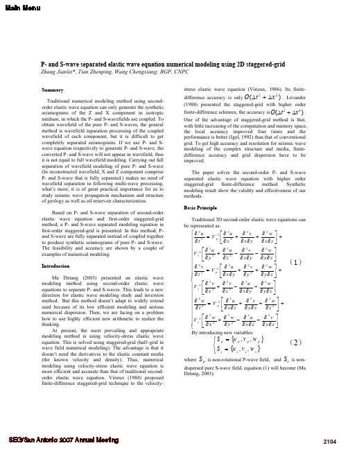
P- and S-wave separate Elastic wave equation numerical modeling using 2D staggered-grid
u = u p + us v = v p + vs w = w p + ws ∂ 2u p ∂t ∂t
u p,vp, wp} S p = { S s = {u s , v s , w s }
(2)Байду номын сангаас
Ss
is non-
where
Sp
is non-rotational P-wave field, and
dispersed pure S-wave field, equation (1) will become (Ma Detang, 2003):
(3)
In order to apply staggered-grid technique, we let ∂ τ xz ∂v x ∂ τ xx + = B ∂z ∂ ∂t x ∂ τ zz ∂v z ∂ τ xz + = B (5) ∂z ∂t ∂x ∂ τ xx ∂v x ∂v z = (λ + 2 µ ) + λ ∂z ∂t ∂x ∂v x ∂v z ∂ τ zz + λ = (λ + 2 µ ) ∂x ∂z ∂t ∂ τ xz ∂v z ∂v x = µ + ∂x ∂t ∂z
Summary Traditional numerical modeling method using secondorder elasti
Laser Ranging to the Moon, Mars and Beyond
a r X i v :g r -q c /0411082v 1 16 N o v 2004Laser Ranging to the Moon,Mars and BeyondSlava G.Turyshev,James G.Williams,Michael Shao,John D.AndersonJet Propulsion Laboratory,California Institute of Technology,4800Oak Grove Drive,Pasadena,CA 91109,USAKenneth L.Nordtvedt,Jr.Northwest Analysis,118Sourdough Ridge Road,Bozeman,MT 59715USA Thomas W.Murphy,Jr.Physics Department,University of California,San Diego 9500Gilman Dr.,La Jolla,CA 92093USA Abstract Current and future optical technologies will aid exploration of the Moon and Mars while advancing fundamental physics research in the solar system.Technologies and possible improvements in the laser-enabled tests of various physical phenomena are considered along with a space architecture that could be the cornerstone for robotic and human exploration of the solar system.In particular,accurate ranging to the Moon and Mars would not only lead to construction of a new space communication infrastructure enabling an improved navigational accuracy,but will also provide a significant improvement in several tests of gravitational theory:the equivalence principle,geodetic precession,PPN parameters βand γ,and possible variation of the gravitational constant G .Other tests would become possible with an optical architecture that would allow proceeding from meter to centimeter to millimeter range accuracies on interplanetary distances.This paper discusses the current state and the future improvements in the tests of relativistic gravity with Lunar Laser Ranging (LLR).We also consider precision gravitational tests with the future laser rangingto Mars and discuss optical design of the proposed Laser Astrometric Test of Relativity (LATOR)mission.We emphasize that already existing capabilities can offer significant improvements not only in the tests of fundamental physics,but may also establish the infrastructure for space exploration in the near future.Looking to future exploration,what characteristics are desired for the next generation of ranging devices,what is the optimal architecture that would benefit both space exploration and fundamental physics,and what fundamental questions can be investigated?We try to answer these questions.1IntroductionThe recent progress in fundamental physics research was enabled by significant advancements in many technological areas with one of the examples being the continuing development of the NASA Deep Space Network –critical infrastructure for precision navigation and communication in space.A demonstration of such a progress is the recent Cassini solar conjunction experiment[8,6]that was possible only because of the use of Ka-band(∼33.4GHz)spacecraft radio-tracking capabilities.The experiment was part of the ancillary science program–a by-product of this new radio-tracking technology.Becasue of a much higher data rate transmission and, thus,larger data volume delivered from large distances the higher communication frequency was a very important mission capability.The higher frequencies are also less affected by the dispersion in the solar plasma,thus allowing a more extensive coverage,when depp space navigation is concerned.There is still a possibility of moving to even higher radio-frequencies, say to∼60GHz,however,this would put us closer to the limit that the Earth’s atmosphere imposes on signal transmission.Beyond these frequencies radio communication with distant spacecraft will be inefficient.The next step is switching to optical communication.Lasers—with their spatial coherence,narrow spectral emission,high power,and well-defined spatial modes—are highly useful for many space applications.While in free-space,optical laser communication(lasercomm)would have an advantage as opposed to the conventional radio-communication sercomm would provide not only significantly higher data rates(on the order of a few Gbps),it would also allow a more precise navigation and attitude control.The latter is of great importance for manned missions in accord the“Moon,Mars and Beyond”Space Exploration Initiative.In fact,precision navigation,attitude control,landing,resource location, 3-dimensional imaging,surface scanning,formationflying and many other areas are thought only in terms of laser-enabled technologies.Here we investigate how a near-future free-space optical communication architecture might benefit progress in gravitational and fundamental physics experiments performed in the solar system.This paper focuses on current and future optical technologies and methods that will advance fundamental physics research in the context of solar system exploration.There are many activities that focused on the design on an optical transceiver system which will work at the distance comparable to that between the Earth and Mars,and test it on the Moon.This paper summarizes required capabilities for such a system.In particular,we discuss how accurate laser ranging to the neighboring celestial bodies,the Moon and Mars,would not only lead to construction of a new space communication infrastructure with much improved navigational accuracy,it will also provide a significant improvement in several tests of gravitational theory. Looking to future exploration,we address the characteristics that are desired for the next generation of ranging devices;we will focus on optimal architecture that would benefit both space exploration and fundamental physics,and discuss the questions of critical importance that can be investigated.This paper is organized as follows:Section2discusses the current state and future per-formance expected with the LLR technology.Section3addresses the possibility of improving tests of gravitational theories with laser ranging to Mars.Section4addresses the next logical step—interplanetary laser ranging.We discuss the mission proposal for the Laser Astrometric Test of Relativity(LATOR).We present a design for its optical receiver system.Section5 addresses a proposal for new multi-purpose space architecture based on optical communica-tion.We present a preliminary design and discuss implications of this new proposal for tests of fundamental physics.We close with a summary and recommendations.2LLR Contribution to Fundamental PhysicsDuring more than35years of its existence lunar laser ranging has become a critical technique available for precision tests of gravitational theory.The20th century progress in three seem-ingly unrelated areas of human exploration–quantum optics,astronomy,and human spaceexploration,led to the construction of this unique interplanetary instrument to conduct very precise tests of fundamental physics.In this section we will discuss the current state in LLR tests of relativistic gravity and explore what could be possible in the near future.2.1Motivation for Precision Tests of GravityThe nature of gravity is fundamental to our understanding of the structure and evolution of the universe.This importance motivates various precision tests of gravity both in laboratories and in space.Most of the experimental underpinning for theoretical gravitation has come from experiments conducted in the solar system.Einstein’s general theory of relativity(GR)began its empirical success in1915by explaining the anomalous perihelion precession of Mercury’s orbit,using no adjustable theoretical parameters.Eddington’s observations of the gravitational deflection of light during a solar eclipse in1919confirmed the doubling of the deflection angles predicted by GR as compared to Newtonian and Equivalence Principle(EP)arguments.Follow-ing these beginnings,the general theory of relativity has been verified at ever-higher accuracy. Thus,microwave ranging to the Viking landers on Mars yielded an accuracy of∼0.2%from the gravitational time-delay tests of GR[48,44,49,50].Recent spacecraft and planetary mi-crowave radar observations reached an accuracy of∼0.15%[4,5].The astrometric observations of the deflection of quasar positions with respect to the Sun performed with Very-Long Base-line Interferometry(VLBI)improved the accuracy of the tests of gravity to∼0.045%[45,51]. Lunar Laser Ranging(LLR),the continuing legacy of the Apollo program,has provided ver-ification of GR improving an accuracy to∼0.011%via precision measurements of the lunar orbit[62,63,30,31,32,35,24,36,4,68].The recent time-delay experiments with the Cassini spacecraft at a solar conjunction have tested gravity to a remarkable accuracy of0.0023%[8] in measuring deflection of microwaves by solar gravity.Thus,almost ninety years after general relativity was born,Einstein’s theory has survived every test.This rare longevity and the absence of any adjustable parameters,does not mean that this theory is absolutely correct,but it serves to motivate more sensitive tests searching for its expected violation.The solar conjunction experiments with the Cassini spacecraft have dramatically improved the accuracy in the solar system tests of GR[8].The reported accuracy of2.3×10−5in measuring the Eddington parameterγ,opens a new realm for gravitational tests,especially those motivated by the on-going progress in scalar-tensor theories of gravity.1 In particular,scalar-tensor extensions of gravity that are consistent with present cosmological models[15,16,17,18,19,20,39]predict deviations of this parameter from its GR value of unity at levels of10−5to10−7.Furthermore,the continuing inability to unify gravity with the other forces indicates that GR should be violated at some level.The Cassini result together with these theoretical predictions motivate new searches for possible GR violations;they also provide a robust theoretical paradigm and constructive guidance for experiments that would push beyond the present experimental accuracy for parameterized post-Newtonian(PPN)parameters(for details on the PPN formalism see[60]).Thus,in addition to experiments that probe the GR prediction for the curvature of the gravityfield(given by parameterγ),any experiment pushingthe accuracy in measuring the degree of non-linearity of gravity superposition(given by anotherEddington parameterβ)will also be of great interest.This is a powerful motive for tests ofgravitational physics phenomena at improved accuracies.Analyses of laser ranges to the Moon have provided increasingly stringent limits on anyviolation of the Equivalence Principle(EP);they also enabled very accurate measurements fora number of relativistic gravity parameters.2.2LLR History and Scientific BackgroundLLR has a distinguished history[24,9]dating back to the placement of a retroreflector array onthe lunar surface by the Apollo11astronauts.Additional reflectors were left by the Apollo14and Apollo15astronauts,and two French-built reflector arrays were placed on the Moon by theSoviet Luna17and Luna21missions.Figure1shows the weighted RMS residual for each year.Early accuracies using the McDonald Observatory’s2.7m telescope hovered around25cm. Equipment improvements decreased the ranging uncertainty to∼15cm later in the1970s.In1985the2.7m ranging system was replaced with the McDonald Laser Ranging System(MLRS).In the1980s ranges were also received from Haleakala Observatory on the island of Maui in theHawaiian chain and the Observatoire de la Cote d’Azur(OCA)in France.Haleakala ceasedoperations in1990.A sequence of technical improvements decreased the range uncertainty tothe current∼2cm.The2.7m telescope had a greater light gathering capability than thenewer smaller aperture systems,but the newer systemsfired more frequently and had a muchimproved range accuracy.The new systems do not distinguish returning photons against thebright background near full Moon,which the2.7m telescope could do,though there are somemodern eclipse observations.The lasers currently used in the ranging operate at10Hz,with a pulse width of about200 psec;each pulse contains∼1018photons.Under favorable observing conditions a single reflectedphoton is detected once every few seconds.For data processing,the ranges represented by thereturned photons are statistically combined into normal points,each normal point comprisingup to∼100photons.There are15553normal points are collected until March2004.Themeasured round-trip travel times∆t are two way,but in this paper equivalent ranges in lengthunits are c∆t/2.The conversion between time and length(for distance,residuals,and dataaccuracy)uses1nsec=15cm.The ranges of the early1970s had accuracies of approximately25cm.By1976the accuracies of the ranges had improved to about15cm.Accuracies improvedfurther in the mid-1980s;by1987they were4cm,and the present accuracies are∼2cm.One immediate result of lunar ranging was the great improvement in the accuracy of the lunarephemeris[62]and lunar science[67].LLR measures the range from an observatory on the Earth to a retroreflector on the Moon. For the Earth and Moon orbiting the Sun,the scale of relativistic effects is set by the ratio(GM/rc2)≃v2/c2∼10−8.The center-to-center distance of the Moon from the Earth,with mean value385,000km,is variable due to such things as eccentricity,the attraction of the Sun,planets,and the Earth’s bulge,and relativistic corrections.In addition to the lunar orbit,therange from an observatory on the Earth to a retroreflector on the Moon depends on the positionin space of the ranging observatory and the targeted lunar retroreflector.Thus,orientation ofthe rotation axes and the rotation angles of both bodies are important with tidal distortions,plate motion,and relativistic transformations also coming into play.To extract the gravitationalphysics information of interest it is necessary to accurately model a variety of effects[68].For a general review of LLR see[24].A comprehensive paper on tests of gravitationalphysics is[62].A recent test of the EP is in[4]and other GR tests are in[64].An overviewFigure1:Historical accuracy of LLR data from1970to2004.of the LLR gravitational physics tests is given by Nordtvedt[37].Reviews of various tests of relativity,including the contribution by LLR,are given in[58,60].Our recent paper describes the model improvements needed to achieve mm-level accuracy for LLR[66].The most recent LLR results are given in[68].2.3Tests of Relativistic Gravity with LLRLLR offers very accurate laser ranging(weighted rms currently∼2cm or∼5×10⁻¹¹in frac-tional accuracy)to retroreflectors on the Moon.Analysis of these very precise data contributes to many areas of fundamental and gravitational physics.Thus,these high-precision studies of the Earth-Moon-Sun system provide the most sensitive tests of several key properties of weak-field gravity,including Einstein’s Strong Equivalence Principle(SEP)on which general relativity rests(in fact,LLR is the only current test of the SEP).LLR data yielded the strongest limits to date on variability of the gravitational constant(the way gravity is affected by the expansion of the universe),and the best measurement of the de Sitter precession rate.In this Section we discuss these tests in more details.2.3.1Tests of the Equivalence PrincipleThe Equivalence Principle,the exact correspondence of gravitational and inertial masses,is a central assumption of general relativity and a unique feature of gravitation.EP tests can therefore be viewed in two contexts:tests of the foundations of general relativity,or as searches for new physics.As emphasized by Damour[12,13],almost all extensions to the standard modelof particle physics(with best known extension offered by string theory)generically predict newforces that would show up as apparent violations of the EP.The weak form the EP(the WEP)states that the gravitational properties of strong and electro-weak interactions obey the EP.In this case the relevant test-body differences are their fractional nuclear-binding differences,their neutron-to-proton ratios,their atomic charges,etc. General relativity,as well as other metric theories of gravity,predict that the WEP is exact. However,extensions of the Standard Model of Particle Physics that contain new macroscopic-range quantumfields predict quantum exchange forces that will generically violate the WEP because they couple to generalized‘charges’rather than to mass/energy as does gravity[17,18]. WEP tests can be conducted with laboratory or astronomical bodies,because the relevant differences are in the test-body compositions.Easily the most precise tests of the EP are made by simply comparing the free fall accelerations,a1and a2,of different test bodies.For the case when the self-gravity of the test bodies is negligible and for a uniform external gravityfield, with the bodies at the same distance from the source of the gravity,the expression for the Equivalence Principle takes the most elegant form:∆a= M G M I 2(1)(a1+a2)where M G and M I represent gravitational and inertial masses of each body.The sensitivity of the EP test is determined by the precision of the differential acceleration measurement divided by the degree to which the test bodies differ(position).The strong form of the EP(the SEP)extends the principle to cover the gravitational properties of gravitational energy itself.In other words it is an assumption about the way that gravity begets gravity,i.e.about the non-linear property of gravitation.Although general relativity assumes that the SEP is exact,alternate metric theories of gravity such as those involving scalarfields,and other extensions of gravity theory,typically violate the SEP[30,31, 32,35].For the SEP case,the relevant test body differences are the fractional contributions to their masses by gravitational self-energy.Because of the extreme weakness of gravity,SEP test bodies that differ significantly must have astronomical sizes.Currently the Earth-Moon-Sun system provides the best arena for testing the SEP.The development of the parameterized post-Newtonian formalism[31,56,57],allows one to describe within the common framework the motion of celestial bodies in external gravitational fields within a wide class of metric theories of gravity.Over the last35years,the PPN formalism has become a useful framework for testing the SEP for extended bodies.In that formalism,the ratio of passive gravitational to inertial mass to thefirst order is given by[30,31]:M GMc2 ,(2) whereηis the SEP violation parameter(discussed below),M is the mass of a body and E is its gravitational binding or self-energy:E2Mc2 V B d3x d3yρB(x)ρB(y)EMc2 E=−4.64×10⁻¹⁰andwhere the subscripts E and m denote the Earth and Moon,respectively.The relatively small size bodies used in the laboratory experiments possess a negligible amount of gravitational self-energy and therefore such experiments indicate nothing about the equality of gravitational self-energy contributions to the inertial and passive gravitational masses of the bodies [30].TotesttheSEP onemustutilize planet-sizedextendedbodiesinwhichcase theratioEq.(3)is considerably higher.Dynamics of the three-body Sun-Earth-Moon system in the solar system barycentric inertial frame was used to search for the effect of a possible violation of the Equivalence Principle.In this frame,the quasi-Newtonian acceleration of the Moon (m )with respect to the Earth (E ),a =a m −a E ,is calculated to be:a =−µ∗rM I m µS r SEr 3Sm + M G M I m µS r SEr 3+µS r SEr 3Sm +η E Mc 2 m µS r SEMc 2 E − E n 2−(n −n ′)2n ′2a ′cos[(n −n ′)t +D 0].(8)Here,n denotes the sidereal mean motion of the Moon around the Earth,n ′the sidereal mean motion of the Earth around the Sun,and a ′denotes the radius of the orbit of the Earth around the Sun (assumed circular).The argument D =(n −n ′)t +D 0with near synodic period is the mean longitude of the Moon minus the mean longitude of the Sun and is zero at new Moon.(For a more precise derivation of the lunar range perturbation due to the SEP violation acceleration term in Eq.(6)consult [62].)Any anomalous radial perturbation will be proportional to cos D .Expressed in terms ofη,the radial perturbation in Eq.(8)isδr∼13ηcos D meters [38,21,22].This effect,generalized to all similar three body situations,the“SEP-polarization effect.”LLR investigates the SEP by looking for a displacement of the lunar orbit along the direction to the Sun.The equivalence principle can be split into two parts:the weak equivalence principle tests the sensitivity to composition and the strong equivalence principle checks the dependence on mass.There are laboratory investigations of the weak equivalence principle(at University of Washington)which are about as accurate as LLR[7,1].LLR is the dominant test of the strong equivalence principle.The most accurate test of the SEP violation effect is presently provided by LLR[61,48,23],and also in[24,62,63,4].Recent analysis of LLR data test the EP of∆(M G/M I)EP=(−1.0±1.4)×10−13[68].This result corresponds to a test of the SEP of∆(M G/M I)SEP=(−2.0±2.0)×10−13with the SEP violation parameter η=4β−γ−3found to beη=(4.4±4.5)×10−ing the recent Cassini result for the PPN parameterγ,PPN parameterβis determined at the level ofβ−1=(1.2±1.1)×10−4.2.3.2Other Tests of Gravity with LLRLLR data yielded the strongest limits to date on variability of the gravitational constant(the way gravity is affected by the expansion of the universe),the best measurement of the de Sitter precession rate,and is relied upon to generate accurate astronomical ephemerides.The possibility of a time variation of the gravitational constant,G,wasfirst considered by Dirac in1938on the basis of his large number hypothesis,and later developed by Brans and Dicke in their theory of gravitation(for more details consult[59,60]).Variation might be related to the expansion of the Universe,in which case˙G/G=σH0,where H0is the Hubble constant, andσis a dimensionless parameter whose value depends on both the gravitational constant and the cosmological model considered.Revival of interest in Brans-Dicke-like theories,with a variable G,was partially motivated by the appearance of superstring theories where G is considered to be a dynamical quantity[26].Two limits on a change of G come from LLR and planetary ranging.This is the second most important gravitational physics result that LLR provides.GR does not predict a changing G,but some other theories do,thus testing for this effect is important.The current LLR ˙G/G=(4±9)×10−13yr−1is the most accurate limit published[68].The˙G/G uncertaintyis83times smaller than the inverse age of the universe,t0=13.4Gyr with the value for Hubble constant H0=72km/sec/Mpc from the WMAP data[52].The uncertainty for˙G/G is improving rapidly because its sensitivity depends on the square of the data span.This fact puts LLR,with its more then35years of history,in a clear advantage as opposed to other experiments.LLR has also provided the only accurate determination of the geodetic precession.Ref.[68]reports a test of geodetic precession,which expressed as a relative deviation from GR,is K gp=−0.0019±0.0064.The GP-B satellite should provide improved accuracy over this value, if that mission is successfully completed.LLR also has the capability of determining PPNβandγdirectly from the point-mass orbit perturbations.A future possibility is detection of the solar J2from LLR data combined with the planetary ranging data.Also possible are dark matter tests,looking for any departure from the inverse square law of gravity,and checking for a variation of the speed of light.The accurate LLR data has been able to quickly eliminate several suggested alterations of physical laws.The precisely measured lunar motion is a reality that any proposed laws of attraction and motion must satisfy.The above investigations are important to gravitational physics.The future LLR data will improve the above investigations.Thus,future LLR data of current accuracy would con-tinue to shrink the uncertainty of˙G because of the quadratic dependence on data span.The equivalence principle results would improve more slowly.To make a big improvement in the equivalence principle uncertainty requires improved range accuracy,and that is the motivation for constructing the APOLLO ranging facility in New Mexico.2.4Future LLR Data and APOLLO facilityIt is essential that acquisition of the new LLR data will continue in the future.Accuracies∼2cm are now achieved,and further very useful improvement is expected.Inclusion of improved data into LLR analyses would allow a correspondingly more precise determination of the gravitational physics parameters under study.LLR has remained a viable experiment with fresh results over35years because the data accuracies have improved by an order of magnitude(see Figure1).There are prospects for future LLR station that would provide another order of magnitude improvement.The Apache Point Observatory Lunar Laser-ranging Operation(APOLLO)is a new LLR effort designed to achieve mm range precision and corresponding order-of-magnitude gains in measurements of fundamental physics parameters.For thefirst time in the LLR history,using a3.5m telescope the APOLLO facility will push LLR into a new regime of multiple photon returns with each pulse,enabling millimeter range precision to be achieved[29,66].The anticipated mm-level range accuracy,expected from APOLLO,has a potential to test the EP with a sensitivity approaching10−14.This accuracy would yield sensitivity for parameterβat the level of∼5×10⁻⁵and measurements of the relative change in the gravitational constant,˙G/G, would be∼0.1%the inverse age of the universe.The overwhelming advantage APOLLO has over current LLR operations is a3.5m astro-nomical quality telescope at a good site.The site in southern New Mexico offers high altitude (2780m)and very good atmospheric“seeing”and image quality,with a median image resolu-tion of1.1arcseconds.Both the image sharpness and large aperture conspire to deliver more photons onto the lunar retroreflector and receive more of the photons returning from the re-flectors,pared to current operations that receive,on average,fewer than0.01 photons per pulse,APOLLO should be well into the multi-photon regime,with perhaps5–10 return photons per pulse.With this signal rate,APOLLO will be efficient atfinding and track-ing the lunar return,yielding hundreds of times more photons in an observation than current√operations deliver.In addition to the significant reduction in statistical error(useful).These new reflectors on the Moon(and later on Mars)can offer significant navigational accuracy for many space vehicles on their approach to the lunar surface or during theirflight around the Moon,but they also will contribute significantly to fundamental physics research.The future of lunar ranging might take two forms,namely passive retroreflectors and active transponders.The advantages of new installations of passive retroreflector arrays are their long life and simplicity.The disadvantages are the weak returned signal and the spread of the reflected pulse arising from lunar librations(apparent changes in orientation of up to10 degrees).Insofar as the photon timing error budget is dominated by the libration-induced pulse spread—as is the case in modern lunar ranging—the laser and timing system parameters do√not influence the net measurement uncertainty,which simply scales as1/3Laser Ranging to MarsThere are three different experiments that can be done with accurate ranges to Mars:a test of the SEP(similar to LLR),a solar conjunction experiment measuring the deflection of light in the solar gravity,similar to the Cassini experiment,and a search for temporal variation in the gravitational constant G.The Earth-Mars-Sun-Jupiter system allows for a sensitive test of the SEP which is qualitatively different from that provided by LLR[3].Furthermore,the outcome of these ranging experiments has the potential to improve the values of the two relativistic parameters—a combination of PPN parametersη(via test of SEP)and a direct observation of the PPN parameterγ(via Shapiro time delay or solar conjunction experiments).(This is quite different compared to LLR,as the small variation of Shapiro time delay prohibits very accurate independent determination of the parameterγ).The Earth-Mars range would also provide for a very accurate test of˙G/G.This section qualitatively addresses the near-term possibility of laser ranging to Mars and addresses the above three effects.3.1Planetary Test of the SEP with Ranging to MarsEarth-Mars ranging data can provide a useful estimate of the SEP parameterηgiven by Eq.(7). It was demonstrated in[3]that if future Mars missions provide ranging measurements with an accuracy ofσcentimeters,after ten years of ranging the expected accuracy for the SEP parameterηmay be of orderσ×10−6.These ranging measurements will also provide the most accurate determination of the mass of Jupiter,independent of the SEP effect test.It has been observed previously that a measurement of the Sun’s gravitational to inertial mass ratio can be performed using the Sun-Jupiter-Mars or Sun-Jupiter-Earth system[33,47,3]. The question we would like to answer here is how accurately can we do the SEP test given the accurate ranging to Mars?We emphasize that the Sun-Mars-Earth-Jupiter system,though governed basically by the same equations of motion as Sun-Earth-Moon system,is significantly different physically.For a given value of SEP parameterηthe polarization effects on the Earth and Mars orbits are almost two orders of magnitude larger than on the lunar orbit.Below we examine the SEP effect on the Earth-Mars range,which has been measured as part of the Mariner9and Viking missions with ranging accuracy∼7m[48,44,41,43].The main motivation for our analysis is the near-future Mars missions that should yield ranging data, accurate to∼1cm.This accuracy would bring additional capabilities for the precision tests of fundamental and gravitational physics.3.1.1Analytical Background for a Planetary SEP TestThe dynamics of the four-body Sun-Mars-Earth-Jupiter system in the Solar system barycentric inertial frame were considered.The quasi-Newtonian acceleration of the Earth(E)with respect to the Sun(S),a SE=a E−a S,is straightforwardly calculated to be:a SE=−µ∗SE·r SE MI Eb=M,Jµb r bS r3bE + M G M I E b=M,Jµb r bS。
Neutrino flux predictions for Galactic plerions

a r X i v :a s t r o -p h /0209537v 1 25 S e p 2002Neutrino flux predictions for galactic plerionsDafne Guetta a ,1&Elena Amato a ,2a INAF/IstitutoNazionale di AstrofisicaOsservatorio astrofisico di Arcetri Largo E.Fermi 5,I–50125Firenze,Italy1IntroductionPlerions are supernova remnants (SNRs)with a filled morphology.These rem-nants are characterized by a center-brightened nebula often seen in the radio and X-ray wavelenghts and believed to be powered by an embedded pulsar.Typified by the Crab Nebula,they have non thermal spectra at all wave-lengths.They have a flat power-law spectral index (α∼0−0.3,S ν∼ν−α)in the radio band and hard photon index (γ∼2,γ=α+1)in the X-ray band.Out of ∼220Galactic SNRs only about 10%are classified as plerions (or Crab-like SNRs)[10].Plerion spectra are usually well interpreted from the radio to the X-ray band as synchrotron emission of a population of relativistic pairs continuously sup-plied by the central pulsar.At higher energies the Inverse Compton Scattering of the same electrons and positrons offeither an internal or external target radiation can play a role.However it is not clear whether this latter processcan be responsible for the emission recently observed from a few objects at TeV energies[16].An alternative mechanism to produce TeV photons may be the decay of neutral pions produced through nuclear collisions of relativistic protons.In this paper we investigate the consequences of a possible hadronic origin of these TeV detections.Following the line of a recent work by Alvarez-Mu˜n iz &Halzen[3],we compute the high energy neutrinoflux at earth andfind that the predictedfluxes may be detectable by large,km2effective area,high energy neutrino telescopes,such as the planned south pole detector IceCube [12]or the Mediterranean sea detectors under construction(ANTARES,[4]; NESTOR,[14])and planning(NEMO,[15];see Ref.[11]for a recent review). 2TeV observations of plerionsFour plerions have been so far detected at TeV energies,while upper limits ex-ist for a few others.The objects for which the detection is at a high confidence level(>∼4σ)are:the Crab Nebula[2],the Vela X SNR[20],the pulsar wind nebula around PSR1706-44[13]and the radio nebula surrounding PSR1509-58[16].The VHE emission is unpulsed and therefore likely to be associated to the pulsar wind nebula rather than to the pulsar magnetosphere.In Table2we report the list of pulsar wind bubbles which have been detected at TeV energies,supplied with the central pulsar luminosity and distance(Ref.[1]and references therein),and the observed TeV spectrum.Two of the objects in the table deserve some comment.First of all,it should be noticed that the association between pulsar B1706-44and the remnant G343.1-2.3is questionable as discussed by Giacani et al.[9],and in the following we refer to the radio nebula detected by Frail et al.[6]as the remnant associated to this pulsar.As to B1509-58,this pulsar is found in a very extended supernova remnant with a complex morphology.However a synchrotron nebula has been found with confidence surrounding the pulsar at X-ray frequencies[17,18,5],although no pulsar wind bubble has been detected at radio frequencies[8].Moreover the spectral index at TeV energies has not been determined with confidence [16].In the following we use a value of2.5in analogy with the spectra of the other objects and derive the normalization from the integrated photonflux measured by CANGAROO.As we mentioned in the introduction,a possible mechanism to interpret the TeVfluxes is the Inverse Compton Scattering(ICS),on the ambient photonTable1Pulsar wind bubbles detected at TeV energies.The name of the pulsar and its associ-ated remnant are reported in thefirst two columns.The pulsar bolometric luminosity and distance from Earth are in the third and fourth column respectively.In the last column the TeV spectrum as given in the references cited above is reported.135SNR dkpcB0531+215 2.8(E/TeV)−2.6Vela.5B1706-440.0340.23(E/1TeV)−2.5MSH15-52 4.4L sync =w CMBTeV 1/2,(2)where Eγis the photon energy.Therefore the synchrotron photons emitted bythe same electrons will have a typical energy of:ǫsync≃0.08B−5keV,(3) where B−5is the nebular magneticfield in units of10−5Gauss.This value of the magneticfield strength is of order of that typically estimated for these nebulae assuming equipartition.If the TeVflux is due to ICS on the CMB,we thenfind for the magneticfield strength:B IC=3×10−6 L x2468L R spectral B eq B ICGHz pc1035erg/sB0531+2110−2−102 1.5150B0833-4510−2−1020.20.12B1706-4410−2−102 1.30.01B1509-58-70.6and Vela a noticeable discrepancy(a factor of4and10respectively)is found. For these two objects the possibility that the TeV emission is due to hadronic processes is particularly appealing.If this is actually the case,then we expect a neutrinoflux from these sources that we compute in the next section.3Neutrino eventsA way to disentangle electromagnetic and hadronic sources of high energy γ-ray emission observationally is to look for the neutrino signals.Relativistic protons may produce TeVγ-rays either by photo-meson production or inelastic nuclear collisions.The relative importance of the two processes depends on the target density of radiation and matter in the source.The main difference,as far as their outcome is concerned,is in the fraction of energy that goes into charged pions compared to neutral ones.This translates in a different ratio between the total neutrino and photon energyflux.In the case of plerions the most likely process at work is p-p scattering,as can be readily seen by comparing the rates of photomeson production and p-p scattering estimated below.For photo-meson production the target for high energy protons is the plerion emission.The fractional energy loss rate of a proton with energy E p(=Γm p c2) due to pion production results in(Ref.[19]):t−1pγ(E p)≃2p+1ǫpeak d4πh≃2.5×10−162p+1R pc2Fνp[mJy]yr−1.(5)Here we have treated the plerion as homogeneous and used the fact that the photon spectrum is a power law,Fν∝ν−p.We have also made the approx-imation that the main contribution to pion production comes from photon energiesǫγ≈ǫpeak=0.3GeV,where the p-γcross section peaks due to the∆resonance.The numerical values are obtained using:σpeak=5×10⁻²⁸cm2,ξpeak=0.2,∆ǫ=0.2GeV,νp=ǫpeak/(Γh)andβp≃1.Finally we have scaled the nebular radius and distance to the typical values of1pc and1kpc,re-spectively(R pc=R N/pc and d kpc=d/kpc),and expressed the nebular synchrotron radiationflux in units of mJy.The energy loss-rate of a relativistic proton due to inelastic nuclear collisionscan be estimated ast−1pp≈ζn tσ0c≈ζM N4πR3Nσ0c,(6)where n t is the target density,which we have expressed in terms of the nebular radius R N and content of thermal material M N.Introducing in Eq.6the numerical values of the cross section for p-p scattering,σ0=5×10⁻²⁶cm2, and of the average fraction of energy lost by the proton,ζ≃20%,we obtain: t−1pp≈10−7M N⊙dEνdEν=E maxγE minγEγdNγdEγ(2Eν)Pνµ(Eν)dEν,(9)where Pνµ=1.3·10−6Eν,TeV[7]is the detection probability for neutrinos with Eν>∼1TeV,T is the observation time and A effis the effective area.The number of atmospheric neutrino events collected in a km2detector during 1yr is of order1.This is estimated assuming a background neutrino spectrumφν,bkg∼10−7E−2.5ν,TeV cm−2s−1sr−1for Eν>1TeV,and a detector angularresolution of0.3◦like NEMO[15].Table3Predicted number of muon events,Nµ,in a km2detector,using Eq.9for the plerions considered in the paper.One year of integration time is assumed.pulsarB0531+21B0833-45B1706-44B1509-58References[1]Aharonian F.A.,Atoyan A.M.,&Kifune T.,1997,MNRAS,291,162[2]Aharonian F.A.,et al.,2000,ApJ,539,317[3]Alvarez-Mu˜n iz J.&Halzen F.,astro-ph/0205408[4]ANTARES Proposal,1997,astro-ph/9707136[5]Brazier K.T.S.&Becker W.,1997,MNRAS,284,335[6]Frail D.A.,Goss W.M.,&Whiteoak J.B.Z.,1994,ApJ,437,781[7]Gaisser T.K.,Halzen F.&Stanev T.,1995,Phys.Rep.,258,173[8]Gaensler B.M.,et al.,1999,MNRAS,305,724[9]Giacani E.B.,et al.,2001,ApJ,121,3133[10]Green D.A.,2001,‘A catalogue of Galactic Supernova Remnants’,(/surveys/snrs)[11]Halzen F.,2001,in Intl.Symp on High Energy Gamma Ray Astronomy,Heidelberg,June2000(astro-ph/0103195)[12]IceCube Proposal,(/a3ri/icecube/overview/original_nsf_proposal)[13]Kifune T.,et al.,1995,ApJ,438,91[14]Monteleoni B.for the NESTOR Collaboration,1996,Proceedings of the XVIIInternational Conference on Neutrino[15]Riccobene G.for the NEMO Collaboration,to appear on the proceedings ofthe“Workshop on methodical aspects of underwater/ice neutrino telescopes”, Hamburg,15-16August2001[16]Sako T.,et al..,2000,ApJ,537,422[17]Seward F.D.,et al.,1984,ApJ,281,650[18]Tamura K.,et al.,1996,PASJ,48,L33[19]Waxman E.&Bahcall J.N.,1997,Phys.Rev.Lett.,78,2292[20]Yoshikoshi T.,et al.,1997,ApJ,487,L65。
Submillimetre-wave surveys first results and prospects

a r X i v :a s t r o -p h /9806369v 211Aug1998Submillimetre-wave surveys:first results and prospects A.W.Blain 11Cavendish Laboratory,Madingley Road,Cambridge,CB30HE,UK.Abstract.The population of distant dusty submm-luminous galaxies was first detected last year [20].Forms of evolution required to account for both this popu-lation and the intensity of background radiation have now been determined [6],and are used to investigate the most efficient observing strategies for future surveys.Submm-wave galaxy surveys detect the redshifted thermal far-infrared ra-diation emitted by dust grains that reprocess optical/ultraviolet light from young stars and active galactic nuclei (AGN).The selection function in red-shift in such surveys is very broad [3],and extends out to redshifts of order 10.Hence they provide an efficient and direct technique for selecting distant dust obscured galaxies and AGN [14].High-redshift biased selection makes submm-wave surveys an ideal way to search for gravitational lenses [2].Consistent models of the evolution of dusty galaxies can be constructed to account for submm counts [1,7,11,13,17,20],mid-infrared counts [15,16]and the submm/far-infrared background radiation intensity [8,10,18,19].While not necessarily correct,these models are well constrained and can be used to predict source counts on a range of different angular scales and at a range of different wavelengths [6].Here the resulting counts are used to investigate the optimal strategies for future mm/submm-wave surveys.The source confusion noise expected in these surveys is discussed elsewhere [4,5].Observed submm-wave counts are presented in Fig.1,alongside the counts predicted by taking an ensemble average of seven different models of galaxy evolution that are consistent with both the observed counts and the inten-sity of background radiation [6].The associated redshift distributions are shown in Fig.2.Excluding [14],no redshifts have yet been determined for submm-selected sources.A spectroscopic redshift distribution of submm-selected sources will provide a powerful test of plausible galaxy evolution mod-els [6].The broad-band colours of the optical identifications in general suggest agreement with the predictions [21].The predicted counts of mm/submm-wave sources can be used to deter-mine the most efficient strategy for detecting distant dusty galaxies,in both general galaxy surveys (Fig.3a)and in surveys for lensed objects (Fig.3b).The detection rate achieved in the crucial first detections using SCUBA will be greatly exceeded in future surveys;for references to suitable instruments see[4].The fraction of lensed sources expected in a survey is shown in Fig.3(c).The rate of confirmation of lenses,including the time required to image lensed structures at sub-arcsec resolution using the MMA,is shown in Fig.3(d).The detection and confirmation rates differ most at faint flux densities,at whichFigure1:Observed source counts and the ensemble mean(thick lines)and1σuncertainty(thin lines)derived from well-fitting count and background models [6].References to the data are B[1],H[11],Hu[13],K[15],La[16],Li[7,17],S[20] and WW[22].Points without a number correspond to850-µm data.the follow-up MMA observations require more time.The detection rates predicted for future instruments[9]and telescopes–an upgraded‘SCUBA+’[12],large ground-based interferometers like the MMA, the50-m LMT,a10-m South Pole telescope and the3.5-m space-borne FIRST –exceed those of SCUBA by up to two orders of magnitude.In concentrated efforts over a number of years,catalogues of order106distant galaxies and AGN will be compiled.Thefine angular resolution of large interferometers will allow the detected sources to be resolved directly in the mm/submm waveband. In some cases,their redshifted mid-infraredfine-structure line emission could be used to determine redshifts directly in the submm waveband.In addition,the cosmic microwave background imaging space mission Planck Surveyor will provide an all-sky arcmin-resolution100-mJy survey,which will be very useful for selecting both extremely luminous submm-wave sources and gravitational lenses[2].•Thefirst detections of distant dusty galaxies indicate that there is an abundant population of such sources.These can be exploited to in-vestigate galaxy formation and evolution,large-scale structure at high redshifts and the values of cosmological parameters.•It is most important to determine the redshift distribution of submm-wave sources selected in blank-field surveys,and thus test thefirst obser-vationally constrained models of the evolution of dust obscured galaxies at high redshifts[6].•Huge samples of distant dusty galaxies and gravitational lenses can be compiled using future instruments–especially the LMT and MMA.Figure2:The ensemble mean(thick lines)and1σuncertainty(thinflanking lines)of predicted submm-selected redshift distributions[6]. Acknowledgements.This work has benefited greatly from SCUBA/JCMT ob-servations in collaboration with Ian Smail,Rob Ivison and Jean-Paul Kneib.I thank Malcolm Longair for helpful comments on the manuscript,and Gislaine Lagache and Dave Clements for discussing the results of the ISO FIRBACK programme.References[1]Barger A.J.et al.,1998,Nat,394,248(astro-ph/9806317).[2]Blain A.W.,1998,MNRAS,297,511(astro-ph/9801098).[3]Blain A.W.&Longair M.S.,1996,MNRAS,279,847.[4]Blain A.W.,Ivison R.J.,&Smail I.,1998,MNRAS296,L29.[5]Blain A.W.et al.,this volume(astro-ph/9806063).[6]Blain A.W.et al.,1998,MNRAS,submitted(astro-ph/9806062).[7]Eales S.A.et al.,1998,ApJL,submitted(astro-ph/9808040).[8]Fixsen D.J.et al.,1998,ApJ,in press(astro-ph/9803021).[9]Glenn J.et al.,in Phillipps T.G.ed.SPIE3357,in press.[10]Hauser M.G.et al.,1998,ApJ,in press(astro-ph/9806129).[11]Holland W.S.et al.,1998,Nat,392,788.[12]Holland W.S.,1998,private communication.[13]Hughes D.H.et al.,1998,Nat,394,241(astro-ph/9806297).[14]Ivison R.J.et al.,1998,MNRAS,298,583(astro-ph/9712161).[15]Kawara K.et al.,1997,in Wilson A.ed.,The Far-Infrared and SubmillimetreUniverse.ESA SP-401,ESA publications,Noordwijk,p.285.[16]Lagache G.et al.,this volume.[17]Lilly S.J.et al.,in press(astro-ph/9807261).[18]Puget J.-L.et al.,1996,A&A,308,L5.[19]Schlegel D.J.et al.,1998,ApJ,499,in press(astro-ph/9710327).[20]Smail I.,Ivison R.J.&Blain A.W.,1997,ApJ,490,L5(astro-ph/9708135).[21]Smail I.et al.,1998,ApJ,submitted(astro-ph/9806061).[22]Wilner D.J.&Wright M.C.H.,1997,ApJ,488,L67.Figure3:Predicted detection rates of unlensed(a)and lensed(b)mm/submm-wave sources at5σsignificance.The rates are uncertain to within a factor of about3.The curves end on the left at aflux density5times the confusion noise[5]and on the right at a count of1/4πsr−1.The fraction of lensed sources(c),and the confirmation rate of lenses(d),after MMA follow-up observations, are also shown.The fraction of lenses is expected to increase at brightflux densities,and to be systematically larger at longer wavelengths.Although the surface density of sources is expected to be small when the lens abundance is greatest,a detection efficiency greater than one per cent should still be achieved in a deeper survey.Lens confirmation rates in(d)were calculated assuming that a850-µm MMA observation10times deeper than the detection threshold is required in order to search for lensed structures in each source.At faintflux densities the time required for these follow-up observations greatly exceeds the time required to carry out the initial survey.Lens surveys should hence be conducted at brighterflux density limits than galaxy surveys.。
MillimetreWaveSu...
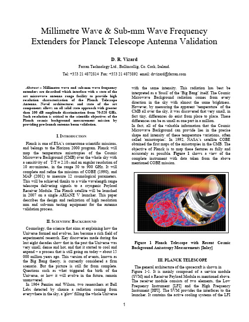
Millimetre Wave & Sub-mm Wave Frequency Extenders for Planck Telescope Antenna ValidationD. R. VizardFarran Technology Ltd , Ballincollig, Co. Cork, Ireland.Tel:+353214872814Fax:+353214873892email:*******************Abstract – Millimetre wave and sub-mm wave frequency extenders are described which interface with a state of the art microwave antenna range facility to provide high resolution characterisation of the Planck Telescope Antenna. Novel architectures and state of the art components allows an all solid state approach with greater than 100 dB amplitude discrimination from 70-320 GHz. Such resolution is critical to the scientific objectives of the Planck cosmic background measurement mission by providing pre-launch antenna beam validation.I. I NTRODUCTIONPlanck is one of ESA’s cornerstone scientific missions, and belongs to the Horizon 2000 program. Planck will map the temperature anisotropies of the Cosmic Microwave Background (CMB) over the whole sky witha sensitivity of T/T = 2.10-6 and an angular resolution of10 arc-minutes, in the range 30 to 900 GHz. It will complete and refine the missions of COBE (1990), and MAP (2001) to measure 12 cosmological parameters. This will be achieved thanks to a wide wavelength range telescope delivering signals to a cryogenic Payload Receiver Module. The Planck satellite will be launched in 2007 on a single ARIANE V launcher. This paper describes the design and realization of high resolution mm and sub-mm testing equipment for the antenna validation process.II. S CIENTIFIC B ACKGROUND Cosmology, the science that aims at explaining how the Universe formed and evolves, has become a rich field of experimental research. Key discoveries made during the last eight decades show that in the past the Universe was very small, dense and hot, and that it started to cool and expand – a process that is still going on today – about 15 000 million years ago. This version of events, known as the Big Bang theory, is currently considered a firm scenario. But the picture is still far from complete. Questions such as what triggered the birth of the Universe, or how it will evolve in the future, remain unanswered.In 1964 Penzias and Wilson, two researchers at Bell Labs detected by chance a radiation coming from everywhere in the sky, a 'glow' filling the whole Universe with the same intensity. This radiation has best be interpreted as a 'fossil' of the ‘Big Bang’ itself. The Cosmic Microwave Background radiation comes from every direction in the sky with almost the same brightness. However, by measuring the apparent ‘temperature’ of the CMB all over the sky, it was discovered that very small, in fact tiny, differences do exist from place to place. These differences can be as small as one part in a million.In fact, all of the valuable information that the Cosmic Microwave Background can provide lies in the precise shape and intensity of these temperature variations, often called 'anisotropies'. In 1992, NASA’s satellite COBE obtained the first maps of the anisotropies in the CMB. The objective of Planck is to map these features as fully and accurately as possible. Figure 1shows a view of the complete instrument with data taken from the above mentioned COBE mission.Figure 1 Planck Telescope with Recent Cosmic Background Anisotropy Measurements [Inlay]III. PLANCK TELESCOPEThe general architecture of the spacecraft is shown in Figure 1-1. It is mainly composed of a service module (SVM) and a Receiver Payload Module as mentioned above. The receiver module consists of two elements, the Low Frequency Instrument [LFI] and the High Frequency Instrument [HFI]. The SVM provides the interfaces to the launcher. It containsthe active cooling systems of the LFIand HFI and satellite control equipment. The LFI and HFI modules operate in nine frequency channels ranging from 30 GHz to 857 GHz.To reach the unprecedented sensitivity goals of the project, the LFI detectors comprising High Electron Mobility Transistors (HEMT) for the 30 to 100 GHz channels and the bolometers for the 100 to 857 GHz channels, are cooled to 20 K and 0.1 K respectively. The detector horns are distributed over the focal surface of an off-axis telescope operating at a temperature between 40 K and 60 K.Figure 1-1 Planck Telescope Showing SVM, Off-axis Antenna, LFI and HFI ModulesThe optics of the telescope is derived from a classical radio frequency antenna design. It is an off-axis Gregorian telescope with two reflectors, a large elliptical primary with dimensions 1.9 x 1.5 m and a smaller elliptical secondary of size 1 x 0.8 m. The wavelength spectral domain ranges from 0.350 mm (857 GHz) to 10 mm (30 GHz). The angular resolution on the sky is better than 13 arcmin for a wavelength of 3 mm (100 GHz).IV. ANTENNA REQUIREMENTSThe aims of the Planck instruments are to obtain an image of the CMB fluctuations and subtract the primordial signal from contaminating astrophysical source of emissions. This can be achieved by excellent control of systematic errors induced by the ‘straylight’. There must be excellent control and verification of the antenna to provide maximum rejection towards specific directions such as the sun, moon and the earth and the self emission of the complete spacecraft. To obtain the required level of characterization the antenna needs to bemeasured over a very wide dynamic range. Additionally given the large antenna diameter compared to the wavelength special facilities are needed to measure the pattern accurately, as discussed briefly below. V. ANTENNA TEST R EQUIREMENTSFor the accurate measurement of the Planck antenna far field patterns including phase it becomes necessary to employ special techniques as the so called ‘far field’ is not developed until a considerable distance from the antenna. In order to accurately measure an antenna’s far zoneperformance, the deviation of the phase of the field across its aperture must be restricted. The criterion generally used is that the phase should be constant to within π/8 radian (22.5°). Under normal operating conditions this criteria is easily achieved since there is usually a large separation between transmitting and receiving antennas. Duringantenna testing however, it is desirable because of various practical considerations to make antenna measurements at as short a range as possible. Generally the range parameter R = 2D 2/lambda is used to define the far field distance, which is over 150 m in the case of a 1.5 metre antenna operating at 100 GHz (3 mm). See Figure 1-2 belowFigure 1-2 Regular Anechoic Chamber VI. C OMPACT ANTENNA TEST RANGEA common technique to avoid the large facility that the above would entail is the use of a Compact Antenna Test Range (CATR) see Fig 1-3. Compact ranges are an excellent alternative to traditional far-field ranges. This method of testing allows an operator to employ an indoor anechoic test chamber at a reasonable cost and avoid problems associated with outdoor range weather and security. In a manufacturing environment, the compactrange can be located near to the final testing and integration facilities. By placing a compact range in a shielded chamber, one can also eliminate interference from external sources.The principle of operation of a compact range is based on the basic concepts of geometrical optics. Diverging spherical waves from a point source located at the focal point of a paraboloidal surface are collimated into a plane wave. This plane wave is incident on the test antenna. The resultant plane wave has a very flat phase front, however the reflector-feed combination introduces a small (but generally acceptable) amplitude taper across the test zone.F1-3VII M ILLIMETRE W AVE I NSTRUMENTATIONTo provide pre-launch antenna verification, amplitude measurements of the main beam and sidelobes with at least 100 dB of dynamic range is required at 70, 100 and 320 GHz. A high level of amplitude and phase stability is required to allow time for the complete measurement of the beam. Additionally the frequency dependence of the antenna is required to be evaluated across the > 2 GHz bandwidth of the operating channels. The transmit and receive modules must fully interface with existing ground support equipment in respect of frequency capability and control software.These requirements have been met by adopting a fully solid state modular approach with 3 TX and 3 RX units. The 70 GHz and 100 GHz units are based on a common LO frequency conversion approach, for convenience of operation with existing equipment. The 320 GHz channel is based on a fixed frequency multiplier chain to provide the maximum possible transmit power and has a separate local oscillator for transmit and receive. Figure 1-4 describes a generic converter arrangement.VII–(A) 70 AND 100 GH Z TX MODULESThe 70 GHz and 100 GHz frequency extenders use a subharmonic mixer based upconversion technique to generate the transmitted test signal. See Figure 1-5. The input drive signal is set to be 3.5 +/- 1 GHz and is provided by the existing microwave equipment. A common TX and RX microwave local oscillator signal is frequency multiplied to provide the final mm-wave mixer LO. A final mm-wave power amplifier provides output power in the range 20-50 mW depending on frequency. A sample of the transmitted power is downconverted in a separate mixing process to provide amplitude compensation for variations caused by frequency or temperature. The advantages of this general approach can be summarised :•Common LO allows use with current GSE equipment and frequency plan•Easy coverage and control of full RF frequency band•Subharmonic mixer approach reduces LO multiplication cost and complexity•Solid state approach has no lifetime or high voltage safety issues•Compact, lightweight and has low power consumptionFigure 1-5 100 GHz TX Module SchematicVII –(B) 70 AND 100 GH Z RX MODULESThe 70 GHz and 100 GHz receiver extenders use a similar subharmonic mixer based downconverter. The output IF signal is now 3.5 +/- 1 GHz and the receiver local oscillator signal provided by multiplication as before. The input noise figure is determined by a low noise MMIC HEMT mm-wave amplifier of typically < 5 dB noise figure. The same general attributes of the TX module apply to the receiver unit. The RX unit is mounted at the antenna under test and is specially packaged to meet the physical constraints imposed at the Planck instrument. 3D models are used to ensure compatibility. Figure 1-6 shows an electrical schematic and Fig 1-7 shows the 100 GHz module mechanical arrangement.Figure 1-6 100 GHz Module Mechanical OutlineVI. S UBMILLIMETRE W AVE I NSTRUMENTATION At 320 GHz the use of an upconverter approach for the transmitter was ruled out due to the restricted outputpower from a mixer upconverter and the lack of power amplifiers for this frequency range. Likewise low noise amplifiers are not available and therefore a direct input mixer receiver was required. The TX module is based on an active frequency multiplier chain starting at 10 GHz with an overall multiplication factor X32, providing an output power of approx 0 dBm. The subharmonically pumped mixer based receiver uses a similar LO chain and has an overall 10 dB noise figure. In order to provide the correct frequency plan independent TX and RX local oscillators are required. The lack of amplifiers for both transmit and receive result in a lower dynamic range, and additionally the antenna is characterised at a fixed frequency only. This is an acceptable trade-off in the application, which can be offset by increasing the integration time used.VIII D EVELOPMENT S TATUSThe frequency extenders described here for the 70-320 GHz frequency range are in the process of manufacture for use in initial antenna testing trials starting May 2005. Development will be complete by Aug 2005 and the first full validation of the Planck antenna at mm and sub-mm wavelengths is expected in late 2005. Examples of previously manufactured custom modules for antenna testing are shown below, in this case for the extension of the ESA CATR facility to provide coverage over 170-260 GHz using similar techniques. Figure 2 details the arrangement.F IGURE 2 170-260 GH Z F REQUENCY EXTENDER MODULESCONCLUSIONSCustom designed mm-wave and sub-mm wave modules for the frequency extension of existing microwave Ground Support Equipment operating within a Compact Antenna Test Range have been described. The modules utilize state of the art mm-wave components including mixers, multipliers, low noise and power amplifiers, and provide an all solid state, compact and reliable solution to the needs of high performance antenna testing through to the sub-mm spectral region.A CKNOWLEDGEMENTS[1] C Nardini, D Drubel, of Alcatel Espace for providingdetails of the Planck telescope testing facility.[2] M Paquay of ESA-ESTEC regarding work done underESA contract.[3] J Coughlan, A O Riordan, Farran Technology Ltd, reProject Management and Mechanical Design.[4] This work is being carried out under contract toAlcatel Espace SA Cannes France。
- 1、下载文档前请自行甄别文档内容的完整性,平台不提供额外的编辑、内容补充、找答案等附加服务。
- 2、"仅部分预览"的文档,不可在线预览部分如存在完整性等问题,可反馈申请退款(可完整预览的文档不适用该条件!)。
- 3、如文档侵犯您的权益,请联系客服反馈,我们会尽快为您处理(人工客服工作时间:9:00-18:30)。
a r X i v :a s t r o -p h /0612612v 1 21 D e c 2006Submitted to the Astronomical JournalPreprint typeset using L A T E X style emulateapj v.12/14/05THE MULTIWAVELENGTH SURVEY BY YALE-CHILE (MUSYC):DEEP NEAR-INFRARED IMAGING ANDTHE SELECTION OF DISTANT GALAXIESRyan Quadri,1Danilo Marchesini,1,2Pieter van Dokkum,1,2Eric Gawiser,1,2,3,4Marijn Franx,5Paulina Lira,3Gregory Rudnick,6C.Megan Urry,2Jos ´e Maza,3Mariska Kriek,5L.Felipe Barrientos,7Guillermo Blanc,8Francisco J.Castander,9Daniel Christlein,1,2,3Paolo S.Coppi,1,2Patrick B.Hall,10David Herrera,1,2Leopoldo Infante,7Edward N.Taylor,5Ezequiel Treister,11Jon P.Willis 12Submitted to the Astronomical JournalABSTRACTWe present deep near-infrared JHK imaging of four 10′×10′fields.The observations were carried out as part of the Multiwavelength Survey by Yale-Chile (MUSYC)with ISPI on the CTIO 4m telescope.The typical point source limiting depths are J ∼22.5,H ∼21.5,and K ∼21(5σ;Vega).The effective seeing in the final images is ∼1.′′0.We combine these data with MUSYC UBV RIz imaging to create K -selected catalogs that are unique for their uniform size,depth,filter coverage,and image quality.We investigate the rest-frame optical colors and photometric redshifts of galaxies that are selected using common color selection techniques,including distant red galaxies (DRGs),star-forming and passive BzKs,and the rest-frame UV-selected BM,BX,and Lyman break galaxies (LBGs).These techniques are effective at isolating large samples of high redshift galaxies,but none provide complete or uniform samples across the targeted redshift ranges.The DRG and BM/BX/LBG criteria identify populations of red and blue galaxies,respectively,as they were designed to do.The star-forming BzKs have a very wide redshift distribution,a wide range of colors,and may include galaxies with very low specific star formation rates.In comparison,the passive BzKs are fewer in number,have a different distribution of K magnitudes,and have a somewhat different redshift distribution.By combining these color selection criteria,it appears possible to define a reasonably complete sample of galaxies to our flux limit over specific redshift ranges.However,the redshift dependence of both the completeness and sampled range of rest-frame colors poses an ultimate limit to the usefulness of these techniques.Subject headings:catalogs —surveys —galaxies:distances and redshifts —galaxies:high-redshift—infrared:galaxies1.INTRODUCTIONThe issues surrounding galaxy formation and evolution provide significant motivation for ongoing astrophysical research.Although several of the basic physical processes that drive the formation and evolution of galaxies were identified some time ago,such as the gravitational col-lapse of dark matter,the cooling and dissipative collapse of baryons,the variation in star formation rates with time,and galaxy mergers,constructing detailed models that reproduce observed properties for a wide range of galaxy types and redshifts has proven exceedingly dif-ficult.A precise determination of the cosmological pa-1Department of Astronomy,Yale University,New Haven,CT Electronic address:quadri@2Yale Center for Astronomy and Astrophysics,Yale University,New Haven,CT3Departamento de Astronom´ıa,Universidad de Chile,Santiago,Chile4National Science Foundation Astronomy and Astrophysics Postdoctoral Fellow5Leiden Observatory,Universiteit Leiden,The Netherlands 6National Optical Astronomical Observatory,Tucson,AZ 7Departamento de Astronom´ıa y Astrof´ısica,Pontifica Univer-sidad Cat´o lica de Chile,Santiago,Chile8Department of Astronomy,University of Texas at Austin,Austin,Texas9Instiut d’Estudis Espacials de Catalunya,Barcelona,Spain 10Department of Physics and Astronomy,York University,Toronto,Canada11European Southern Observatory,Santiago,Chile12Department of Physics and Astronomy,University of Victoria,Victoria,Canadarameters has removed some of the uncertainties,but it is largely accepted that comprehensive observations of galaxies at low and high redshifts are necessary to refine our understanding of galaxy evolution.Recent years have seen dramatic progress in the obser-vational study of high redshift galaxies.Much of this progress has been driven by deep imaging of “blank”fields with multiple bandpasses.These surveys often rely on carefully-designed color selection techniques,mak-ing use of only a few bands,to isolate samples of high redshift galaxies.The most well known color selection criteria identify the Lyman Break Galaxies (LBGs)at z ∼3(Steidel et al.1996),using the U n GR bands.This technique has been extended to select LBGs at higher redshifts,and to select similar star-forming galaxies at z ∼2.3and z ∼1.7(BX and BM galaxies,respectively;Adelberger et al.2004).Selecting galaxies in optical bands may miss many red high redshift galaxies,so NIR selection techniques have also become important.Ex-tremely Red Objects (EROs)are at z 1,and have been selected using a variety of criteria,such as R −K >5and I −H >3(McCarthy 2004).Franx et al.(2003)used J −K >2.3to select distant red galaxies (DRGs)at z ∼2−4.Daddi et al.(2004)proposed a technique involving the BzK bands to identify galaxies at z >1.4.Yan et al.(2004)used (z −3.6µm)AB >3.25to isolate IRAC Extremely Red Objects (IEROs).The primary advantage of such selection techniques is that they rely on only a few observed bands to isolate2Quadri et al.large samples of galaxies in a(hopefully)well-defined red-shift range.However,diagnostic information about indi-vidual galaxies or about the range of properties spanned by a sample of galaxies requires more bands to trace the detailed spectral energy distributions over a wide wave-length range.Specific color selection techniques may also identify only a subset of galaxies in the targeted redshift range(by design),offering a limited view of the diver-sity of galaxy properties at that redshift.Surveys with a large number of observed bands may be able to use photometric redshifts to obtain a more complete sample of galaxies in any given redshift range,and are better able to specify the intrinsic properties of high redshift galaxies.With these issues in mind,we have executed a deep op-tical/NIR survey of four southern and equatorialfields as part of the Multiwavelength Survey by Yale-Chile (MUSYC).13Subsets of these data have been used to study several characteristics of K-selected galaxies at z>2,including the number density and colors of mas-sive galaxies(van Dokkum et al.2006),the clustering properties(Quadri et al.2006),and the luminosity func-tion(Marchesini et al.2006).Additionally,Kriek et al. (2006a,b,c)obtained NIR spectroscopy of the brightest MUSYC galaxies,and Webb et al.(2006)used Spitzer MIPS imaging to infer the star formation rate of MUSYC DRGs.The purpose of this paper is two-fold.First,we present the MUSYC deep NIR imaging.We describe the ob-servations,data reduction,and the K-selected catalogs with full UBV RIzJHK photometry.Second,we use these catalogs and high quality photometric redshifts to investigate the properties of galaxies that are selected with common color selection criteria.We use Vega mag-nitudes unless noted otherwise.Throughout we use H0=70km−1s−1Mpc−1,Ωm=0.3,andΩΛ=0.7.2.THE MULTIW AVELENGTH SURVEY BY YALE-CHILE The MUSYC survey consists of several components: optical imaging of four30′×30′fields,NIR imag-ing over the same area,deeper NIR imaging over four 10′×10′subfields,and spectroscopic followup.Some of the MUSYCfields also benefit from imaging by Chandra and XMM in the x-ray,HST in the optical,and Spitzer in the infrared.The survey design is described by Gawiser et al. (2006a).The four30′×30′fields were selected to have low Galactic reddening,HI column density(Burstein& Heiles1978),and100µm dust emission(Schlegel et al. 1998).They were also chosen to have high Galactic lat-itude to reduce the number of stars,to cover a wide range in right ascension to enableflexible scheduling, and to be accessible from Chilean observatories.These fields were observed with UBV RIzfilters for complete optical coverage.A narrowband5000˚Afilter was also used to identify Lymanαemitters at z≃3(Gawiser et al.2006b).Gawiser et al.(2006a)presents images and optically-selected catalogs of one of the MUSYCfields, EHDF-S.The full optical data for the remainingfields will be described elsewhere(E.Gawiser et al.2007,in preparation).The four30′×30′fields were also observed in at least 13/MUSYC one of the J,H,and K bands.We refer to this as the “wide”portion of the MUSYC NIR imaging.These data were collected and processed in a similar way to the data described in this paper(E.Taylor et al.2007,in prepa-ration;G.Blanc2007et al.2007,in preparation).The typical depths are J∼22.and K∼20.Four10′×10′subfields were observed to greater depth in all of JHK.These data,which are referred to as the “deep”NIR MUSYC imaging,are presented in this pa-per.Two of these subfields,HDFS1and HDFS2,are adjacent and lie within the larger30′×30′MUSYC Ex-tended Hubble Deep Field-South(EHDF-S).The other two subfields lie within the larger MUSYC1030and1255fields.We did not perform deep NIR imaging in the fourth large MUSYCfield,ECDF-S,because very deep imaging in the central region of thisfield has been made available by the Great Observatories Origins Deep Sur-vey(GOODS)team(Giavalisco et al.2004).The exact locations of the deep MUSYCfields within the larger 30′×30′fields were chosen to avoid bright r-mation about thesefields is given in Table1.3.OBSERVATIONSThe MUSYC deep NIR observations were performed with the Infrared Sideport Imager(ISPI)(Probst et al. 2003;van der Bliek et al.2004)on the CTIO Blanco 4m Telescope.The detector is a2048×2048HgCdTe HAWAII-2array,with a∼0.′′305pixel scale and a10.′5×10′.5field of view.Observation were performed over the course of9observing runs from January2003to April 2006.The mean airmass of observation varied between1.21 and1.43for differentfield/filter combinations,and ex-posures were rarely taken at airmass>1.6.Standard stars from Persson et al.(1998)were observed2-4times per night except when the conditions were poor.The range of airmass values for standard star observations was similar to that of science observations.The background emission in the NIR is bright, non-uniform across thefield,and can vary on short timescales.Accurate background subtraction requires that the telescope be dithered between exposures(see §4).Because the brightest objects in an exposure can leave residual images in subsequent exposures,using a non-regular dither pattern–in which the telescope does not repeatedly trace the same sequence of dither posi-tions–facilitates removal of artifacts during the reduc-tion process.We used an algorithm to generate semi-random dither patterns in which the distance between subsequent dither positions is maximized.The size of the dither box is45′′,which is sufficiently large to ob-tain good background subtraction in the regions around all but the brightest/most extended sources in ourfields without significantly reducing the area with the highest exposure times.The typical exposure times at each dither position were 1×100s(coadds×individual exposure time)in J,4×20s in H,and4×15s in K.The total exposure times for eachfield/filter combination,after discarding images with poor quality(§4),are given in Table1.The set offilters used with ISPI changed in April2004. Thefields HDFS1and1030were completed using the original JHK′filters,whereas HDFS2and1255were ob-served using the newer JHK sfilters.Both sets offilterDeep NIR Imaging from the MUSYC Survey3Fig. 1.—The filter transmission curves,including atmospheric transmission,used for the MUSYC NIR imaging.The solid curves are for HDFS1and 1030and the dashed curves are for HDFS2and 1255.transmission curves are shown in Figure 1.Conversions between the Vega and AB magnitude systems were cal-culated using the SED of Vega,and are given,along with the effective wavelengths,in Table 2.Note that the shift in effective wavelength between the K ′and K s filters is small,and much less than the filter widths.In the dis-cussion that follows we do not distinguish between the two filter sets.4.DATA REDUCTION AND IMAGE PROPERTIES4.1.Data ReductionThe data were reduced using a combination of stan-dard IRAF 14tasks,modified IRAF tasks,and custom tasks.The core of our reduction procedure was the ex-ternal IRAF package XDIMSUM.15The basic methods are similar to those described in detail by Labb´e et al.(2003),and are outlined below.Near-infrared cameras have a non-negligible dark cur-rent,so dark images with the appropriate exposure time and number of coadds are subtracted from the science images.We use domeflats to perform the flat field cor-rection.To remove the background emission from the domeflat image,and thus to isolate the uniform illumina-tion of the dome screen by the lamp,we follow the stan-dard procedure of subtracting a “lamp off”image from a “lamp on”image.During the observations,special care was taken to keep the count level of the “lamp on”im-ages at a reasonable level,well below where non-linearity becomes significant on the ISPI camera.Domeflats were taken nightly or semi-nightly;they were generally sta-ble from night to night,but showed significant variations between observing runs.14IRAF is distributed by the National Optical Astronomy Ob-servatories,which are operated by the Association of Universities for Research in Astronomy,Inc.,under cooperative agreement with the National Science Foundation.15/iraf/ftp/iraf/extern-v212/xdimsum020806The background emission in each science frame is subtracted,and the resulting images combined,in two passes.During the first pass,an image of the back-ground emission is created for each science image using a running median of the dithered sequence of science im-ages;e.g.the background for image 10is the median combination of images 6-9and 11-14.The positions of several stars are used to determine the relative shifts be-tween background-subtracted images.The images are shifted to a common reference using sub-pixel interpo-lation and are combined.Objects in the combined im-age are detected using a simple thresholding algorithm.These masks are shifted back into the frame of individual science exposures,and the background-subtraction pro-cess is repeated during the second pass;this time objects are masked out during the calculation of the running me-dian in order to improve the background subtraction.We take several steps to improve the quality of the final images.We create a mask of bad pixels in each image.An initial list of bad pixels is created using the flat-field images.We then inspect each background-subtracted image individually;images with severe ar-tifacts (e.g.disturbed point spread functions)are dis-carded,while others with localized artifacts (e.g.satellite trails)are masked using a custom procedure.Additional bad pixels in each image are identified using a cosmic ray detection procedure or are removed with a sigma-clipping algorithm during image combining.The ISPI array can retain memory of previous exposures in the form of persistence images of bright objects.We create a second object mask at the end of the first pass reduc-tion,in which only the cores of the brightest objects are masked;these are used to mask the pixels that contained bright objects during the previous exposure.Finally,we optimize the signal-to-noise in the seeing disk by using a weighted average during the final image combining step.The weights are calculated usingw i =14Quadri et al. We use the IRAF tasks GEOMAP and GEOTRANto re-sample the NIR images so that they follow thesame logical and world coordinate system(i.e.x,ypixel coordinates and RA,Dec)as a set of trimmed op-tical MUSYC images.This processflips the NIR imagesaround the x-axis so that North is up and East is left,in accordance with standard practice.The pixel scale is changed slightly,from0.′′305to0.′′267.We used a6th or-derfit in x and y,allowing for cross-terms,to adequatelyremove the distortions present in the ISPI instrument;a similar high-orderfit was also found to be necessaryby ISPI instrument scientists16.We verified that thepixel resampling does not introduce systematic errors influx for a set of objects distributed across the images.The rms error in stellar positions between the NIR andoptical images is∼0.′′06,much smaller than the typical aperture size used for photometry.We also comparedthe positions of stars in our K-band images to those inthe USNO-B catalog directly.Many of the objects are infact extended,and some others are saturated in our im-ages;after removing these objects the rms is0.′′15−0.′′2, consistent with the uncertainties of individual USNO-Bstars.Thefinal K-band images are shown in Figure2.Thestretch has been adjusted to emphasize faint sources andthe uniformity of the background.Figure3shows a color composite image of HDFS1,constructed using the RJK bands.The effective seeing in thefinal images is takenas the median of the FWHM for a set of∼5−10stars,and is given in Table1.4.3.Photometric Calibration and Verification Observations of standard stars from Persson et al. (1998)were performed nightly except when the condi-tions were very poor.Each standard star observationused a large5-point dither pattern,and the telescopewas de-focused to keep the peak count level in the linearregime of ISPI.Following Persson et al.(1998),the in-strumental magnitude of the star was measured in a10′′diameter aperture;we verified that increasing the aper-ture size would change the instrumental zeropoints by<1%.The zeropoint rms from a single dither sequenceof a standard star is typically0.01−0.03,setting an ap-proximate scale for theflatness of the images.We then calibrated a set of secondary standard stars in the sciencefield with the same size aperture,after applying a small correction for the different airmass of standard star andscience observations.It was not possible to determine ac-curate airmass coefficients from our observations,so weused the coefficients given by Frogel(1998),which were nonetheless found to be consistent with our observations. Following usual practice in the NIR,we did not accountfor color terms in the photometric calibration.There was at least one night for eachfield/filter com-bination where the observing conditions were sufficientto determine an accurate calibration of the secondary standards.Forfield/filter combinations where there wasmore than one night of satisfactory calibrations,the agreement between nights is typically0.01−0.02.Whileit is difficult to place constraints on possible systematic uncertainties,the internal precision of ourfinal zero-points is 0.03in every case.The zeropoints are given16see /instruments/irDeep NIR Imaging from the MUSYC Survey5Fig.2.—The deep K-band images from the MUSYC.At top,the individual HDFS1and HDFS2images have been combined to create a single19.′5×10.′3image.The otherfields are∼10.′3on a side.zeropoints using2MASS photometry;but without otherdata to compare with,we cannot be certain that our0.03magnitude zeropoint uncertainties for thesefieldsare reliable.4.4.Noise Properties and Limiting DepthsTheflux uncertainty within an aperture has a con-tribution from the photon statistics from astronomicalobjects,as well as a contribution from background noise,which is due to sky emission,read noise,etc.The stan-dard method of determining the contribution of back-ground noise,by e.g.SExtractor(Bertin&Arnouts1996)or the APPHOT package of IRAF,is to scalethe rmsflux value of background pixels by the squareroot of the number of pixels within the aperture,6Quadri etal.Fig.3.—An RJK composite of HDFS1.Figure 5shows how the width of the best-fitting Gaussian changes with aperture size,along with predictions from theGAIN,(2)where F is the flux in ADU,GAIN is the total effec-tive gain,and σback is estimated for an aperture with the appropriate size.In the case of the elliptical Kron aper-tures (see §5)we estimate σback for a circular aperture with the same area.The characteristics of the final images can be found in Table 3.This table includes an estimate of the 5σpoint source limiting depths.These values are calculated using the background fluctuations in the color aperture (see §5.3),and with a 0.75magnitude aperture correction applied to account for the ∼50%point-source flux that falls outside this aperture.An alternate analysis of the limiting depths can be found in §5.5.5.SOURCE DETECTION AND PHOTOMETRY5.1.Source DetectionWe used the SExtractor v2.4.3software (Bertin &Arnouts 1996)to detect objects in the K -band im-ages.The two parameters that affect the sensitivity of source detection are DETECTMINAREA,Deep NIR Imaging from the MUSYC Survey7Fig. 4.—Histograms of backgroundfluctuations in1.′′5and2′′diameter apertures in the HDFS1K-band image.The largeraperture has the broader distribution offluxes.The dashed curvesare the best-fittingGaussians.Fig. 5.—The rms value of backgroundfluctuations within anaperture as a function of the aperture size for HDFS1K.Thefilled circles illustrate the measured values,while the solid curveis a power lawfit.The dashed curves show the expected scalingfrom the measured pixel-to-pixel rms relation in the case of no pixelcorrelations(lower)and perfect correlation of all pixels within eachaperture(upper).which specifies the number of adjacent pixels that mustmeet this threshold.Additionally,SExtractor option-allyfilters the detection image with a convolution ker-nel prior to detection in order to enhance the detec-tion of faint objects.Rather than use detailed simula-tions tofind the optimum set of parameters for SEx-tractor,we made use of the ultradeep K-band imageof HDFS from the public FIRES survey(Labb´e et al.2003).The difference in depth between the MUSYCHDFS1K-band image and the FIRES HDF-S image(K∼21.0and K∼24.3,respectively)allows for aclear determination of which objects detected by SEx-tractor in HDFS1are real and which are noise peaks.We increased the DETECTMINAREA=5pixelsand DETECT8Quadri et al.We use SExtractor in dual-image mode to detect ob-jects in K and to perform photometry in all bands.In this subsection we describe our methods to determine “total”flux in K,and to measure high signal-to-noise (S/N)colors.The totalflux in any other band can be calculated directly from these quantities.We estimate the total K-bandflux of an object from the SExtractor AUTO photometry,which uses aflexible elliptical Kron-like aperture.Although this aperture con-tains most of theflux for bright objects,in practice the aperture can become quite small for faint sources–even for the same light profile–so a larger fraction of light may be missed.Therefore we convert the AUTOflux to total flux by applying an aperture correction.The aperture correction is calculated using the median stellar growth curve of a set of bright stars,for a circular aperture with the same area as the AUTO aperture.We note that this procedure may introduce a mild bias in the total flux of faint,extended sources,because their light pro-files may not follow that of a point source outside the AUTO aperture;however these sources will have highly uncertainflux measurements no matter what procedure is used.The aperture correction for the AUTO aper-ture can reach∼0.5magnitudes for some of the faintest sources.Because accurate color measurements are necessary for photometric redshift calculations and modeling of stel-lar populations,we wish to optimize the S/N.Since the noise is a strong function of aperture size(Fig.5),we measure the colors in smaller apertures than the AUTO aperture that is used to estimate the totalflux.For a point source with a Gaussian PSF,and for uncorrelated background noise,the aperture with optimal S/N has diameter1.35×F W HM(Gawiser et al.2006a).In real-istic situations there are competing effects which change the size of the optimal aperture.Relative to the ideal-ized case,the broader wings of our PSFs would suggest a larger aperture to obtain the same signal,while the noise correlations suggest a smaller aperture to keep the same level of noise.The optimal S/N aperture for a point source can be found by dividing the stellar growth curve by theσback curve shown in Figure5.Wefind that the optimal aperture typically has diameter∼1.1−1.4times the FWHM,depending on thefilter(see also Gawiser et al.2006a).Using a very small aperture for color deter-minations presents several problems.Accurate colors re-quire that a similar fraction of theflux from an object is contained within the color aperture in eachfilter,which is easier to achieve with larger apertures.This is because a larger aperture contains a larger fraction of theflux, leading to a smaller relative difference in the fraction of flux.Secondly,one of the primary scientific goals of the deep NIR MUSYC survey is the study of high redshift galaxies,which may not appear as pure point-sources in our∼1′′rger apertures also reduce the effects of the small variations in PSF across the images,and the residual geometric distortions at the edges of the images. We choose,as a compromise,apertures with diameter ∼1.5times the stellar FWHM.These apertures contain ∼50%of the light from a point source.We verified that the S/N in these apertures is 95%of the S/N in the optimal aperture for every image.5.4.Catalog formatThe photometry in the K-selected catalogs is presented in units offlux,normalized so that the zeropoint is25on the AB system.The use offlux,rather than magnitudes, avoids the problem of converting the measuredflux un-certainties into magnitude uncertainties,the problem of asymmetric magnitude uncertainties for low S/N objects, and the loss of information for objects that have nega-tive measuredfluxes.The photometry is not corrected for Galactic extinction.Object detection and measurement of geometrical parameters are performed by SExtractor in the rms-normalized K image.The adjacent HDFS1and HDFS2fields were treated separately,but a list of objects that appears in both catalogs is available.Version3.1of the K-selected catalogs are given in the following format: Column1:SExtractor ID number,starting with1 Columns2-3:x and y barycentersColumns4-5:RA and DEC(decimal degrees;J2000) Column6:internal MUSYCfield code(4=HDFS1, 5=HDFS2,6=1030,7=1255)Columns7-24:Flux density and uncertainty in the color aperture,in the order UBV RIzJHKColumns25-26:K-bandflux density and uncertainty in the“total”apertureColumns27-35:Exposure time weight in bands UBV RIzJHK,normalized to the weight of the median objectColumns36-37:Diameters of color and AUTO aper-tures.The diameter of the AUTO aperture is taken as the geometric mean of the major and minor axes(arcsec) Columns38:SExtractor blendingflag2–object was originally blended with another object(1=blended, 0=unblended)Columns39:SExtractor blendingflag1–object was blended with another object strongly enough to sig-nificantly bias AUTO photometry(1=blended,0=un-blended)Column40:Half-light radius(arcsec)Column41:EllipticityColumn42:Position angle(degrees),measured counter-clockwise from NorthColumn43:Aperture correction to convert AUTOflux to totalfluxColumn44:SExtractor CLASSDeep NIR Imaging from the MUSYC Survey9 Fig. 6.—The K-band completeness curves.Point sourceswere inserted at random locations in the central region of the fourMUSYCfields,where the exposure time is 95%of the total.Thecompleteness is defined as the fraction of simulated sources thatwere recovered,as a function of total magnitude of the simulatedsource.The completeness values are higher if the simulated pointsources are inserted in empty regions of the images(see Table4).blend them.This effect causes the plateau in the com-pleteness curves at brighter magnitudes to have someslope;evidently,this problem is worse at fainter mag-nitudes.We repeated the simulations,this time insert-ing point sources in locations that avoid other(real orsimulated)objects.The completeness is now equal tounity to at least K=20.5in allfields.Table4showsthe90%and50%completeness limits for the deep K-selected MUSYC catalogs for both the“unmasked”and“masked”simulations.We note that the completeness limits from the un-masked and masked simulations are similar,reflectingthe uncrowded nature of thefields to our depth in K.The masked simulations may provide a better estimateof the sensitivity of our images,while the unmasked(shallower)simulations should be used when assessingthe completeness for actual astronomical objects becausesuch objects do not avoid each other on the sky.We alsonote that the completeness for extended objects will belower than for the simulated point sources,and would inprinciple be a function of inclination,morphology,andsize.6.NUMBER COUNTSFigure7shows the surface density of objects as a func-tion of magnitude,excluding objects classified as stars(§7),for each of our fourfields.No completeness correc-tions have been applied.The number counts are calcu-lated in0.5magnitude bins using only the image areawith>95%of the total K-band exposure time.Theerrorbars assume Poisson statistics,which should un-derestimate the true uncertainties because objects areclustered.The fourfields are generally consistent over18 K 20,where the S/N is high and differences indepth do not affect the number counts.It is noteworthythat the1030field has the highest density of objects inthis magnitude range;thisfield also has the highest den-sity of galaxies with M>1011M⊙at2<z phot<3of anyof thefields studied by van Dokkum et al.(2006),sug-gesting the possibility of significant galaxy over-densitiesin this redshift range.The upper panel of Figure8shows the average num-ber counts of the fourfields,along with counts drawnfrom the literature.The completeness corrections de-scribed above have been applied to the MUSYC points.Note that these completeness values provide a simplis-tic correction when dealing with number counts;a moresophisticated correction would account for the differencebetween the measured and intrinsic magnitudes of theartificial sources.This can be a significant effect be-cause the rising slope of number counts means that moresources would scatter to brighter magnitudes than tofainter magnitudes due to noisefluctuations.Further-more,there may be biases in the photometry of thefaintest sources(see also F¨o rster Schreiber et al.2006).Neither do we attempt to correct for spurious detections,which would only be significant at the faintest magni-tudes,or estimate completeness correction for extendedsources.For these reasons we only extend the averagenumber counts to the bin centered at K=21,where thecompleteness correction begins to become significant.The bestfit logarithmic slope d(logN)/dM to theMUSYC number counts isα≈0.31over18≤K≤20.To illustrate deviations from this power law in differentmagnitude ranges,in the lower panel of Figure8we havedivided the observed number counts by thisfit.The de-viation from unity in this panel at brighter magnitudesillustrates a change in the d(logN)/dM relation.How-ever,we do notfind evidence for a sharp break in thepower law slope at K∼17.5,as has been reported byCrist´o bal-Hornillos et al.(2003).These authors interpretthe galaxy number counts in terms of models of galaxyevolution,and suggest that the break can be reproducedby models with late star formation in massive galaxies(z 2;see also Eliche-Moral et al.2006).There is alsosome evidence from deeper surveys that the slopeflattensat K 21;for instance,the data of F¨o rster Schreiber etal.(2006)indicateα≈0.20over21≤K≤23.7.PHOTOMETRIC REDSHIFTS AND STARCLASSIFICATIONWe calculate photometric redshifts using the methodsdescribed by Rudnick et al.(2001,2003).Briefly,non-negative linear combinations of galaxy templates arefitto the observed spectral energy distributions.The tem-plates include the four empirical templates of Coleman,Wu,&Weedman(1980)and the two empirical star-burst templates of Kinney et al.(1996),all of which havebeen extended into the UV and NIR using models.Wealso include10Myr and1Gyr old single stellar populationtemplates generated with the Bruzual&Charlot(2003)models,as the empirical templates are derived from low-redshift galaxies and do not adequately describe some ofthe high-redshift galaxies in the MUSYC catalogs.Wedo not allow for additional reddening in the models.Thephotometric redshift uncertainties are calculated usingMonte Carlo simulations,in which the observedfluxesare varied within the photometric uncertainties.We cor-rected for Galactic extinction when calculating photo-metric redshifts(Schlegel et al.1998).。