Introduction of Finite Element Method-Lesson3
P1有限元方法(P1-FEM)

Let Uh =
i=1
ai ϕi
(VP)become: Find Uh Vh ,such that : a(Uh , ϕi ) = F (ϕi ) i.e.
N −1 i=1
proof : Notice that a(u − uh , vh ) = F (vh ) − F (vh ) = 0,we get, a(u − uh , u − uh ) = a(u − uh , u − vh + vh − uh ) = a(u − uh , u − vh ) ≤ α||u − uh ||V ||u − vh ||V Further, 2 a(u − uh , u − uh ) ≥ γ ||u − uh ||V it leads to ||u − uh ||V ≤ α γ infvh Vh ||u − vh ||V This theorem tells us that uh is a good approximate solution of u in Vh
2.3
P1-Finite Element Method
There is an natural quetion:How to choose Vh . A simple idea is that let Vh be a set of continuous piecewise linear functions which satisfy the boundary condition.
2.2
Garlekin Method
In reality,the space V always has infinite dimension.As a result,numerical method can not be used to find the exact answer in V.The main idea of Galerkin method is that find the approximate solution of u in Vh which is the subspace of V and with finite dimension. i.e. Find uh Vh s.t a(uh , vh ) = F (vh ) for all vh Vh 2 (GM)
一维有限单元法
一维有限单元法
一维有限单元法(Finite Element Method,FEM)是一种数值分
析技术,用于解决求解复杂非线性有限定义域内的热传导,弹性以及
磁学问题。
它是一种有效的计算方法,用于处理各种物理和化学的非
线性变分问题,是工程计算的重要工具。
FEM的基本思想是将一个求解结构用有限个几何元素组成,每个
几何元素都被抽象为若干个结点,考虑元素间的位置和连接关系,有
限个结点之间的运动被模拟,研究得到各个节点、区域或整体的操作
状态。
FEM的步骤是:(1)网格划分,将复杂的物体分割成有限的单元组成;(2)拟态函数建模,用有限二次函数对实体解除近似;(3)全局组装,统一表达各种非线性矩阵方程;(4)求解和分析,建立模
型进行求解分析,实际是求解有限元方程组。
FEM还可以用于解决流体力学中的大循环Navier-Stokes方程,
以及岩土力学中的弹性变形分析和破坏问题。
FEM也可以用于求解有
限定义域内多维问题。
这里可以把三维空间划分为空间相关的几何元
素组成,然后运用FEM展开计算和分析。
从近年来FEM发展势头来看,FEM将继续受到广泛的关注和重视,因为它能够解决科学和工程方面繁复复杂的实际问题,为工程优化提
供造价高效的、可靠的分析方法。
有限元分析基础
第一讲第一章有限元的基本根念Basic Concepts of the Finite Element Method1.1引言(introduction)有限元(FEM或FEA)是一种获取近似边值问题的计算方法。
边值问题(boundary value problems, 场问题field problem )是一种数学问题(mathematical problems)(在所研究的区域,一些相关变量满足微分方程如物理方程、位移协调方程等且满足特定的区域边界)。
边值问题也称为场问题,场是指我们研究的区域,并代表一种物理模型。
场变量是满足微分方程的相关变量,边界条件代表场变量在场边界上特定的值(物理边界转化为数学边界)。
根据所分析物理问题的不同,场变量包括位移、温度、热量等。
1.2有限元法的基本思路 (how does the finite element methods work)有限元法的基本思路可以归结为:将连续系统分割成有限个分区或单元,对每个单元提出一个近似解,再将所有单元按标准方法组合成一个与原有系统近似的系统。
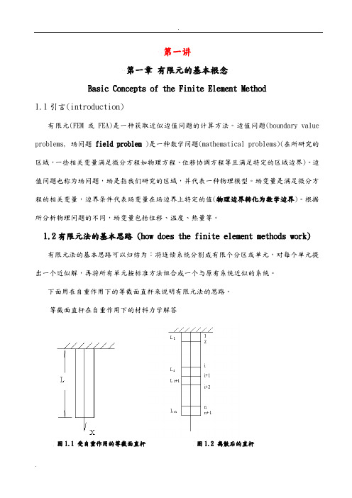
下面用在自重作用下的等截面直杆来说明有限元法的思路。
等截面直杆在自重作用下的材料力学解答图1.1 受自重作用的等截面直杆图1.2 离散后的直杆受自重作用的等截面直杆如图所示,杆的长度为L ,截面积为A ,弹性模量为E ,单位长度的重量为q ,杆的内力为N 。
试求:杆的位移分布,杆的应变和应力。
)()(x L q x N -=EAdx x L q EA dx x N x dL )()()(-== ⎰-==xx Lx EA q EA dx x N x u 02)2()()( (1))(x L EAq dx du x -==ε )(x L A q E x x -==εσ 等截面直杆在自重作用下的有限元法解答(1)离散化如图1.2所示,将直杆划分成n 个有限段,有限段之间通过一个铰接点连接。
称两段之间的连接点为结点,称每个有限段为单元。
有限单元法基本原理与数值方法
有限单元法基本原理与数值方法英文回答:Basic Principles of Finite Element Method.The finite element method (FEM) is a numerical technique used to find approximate solutions to boundary value problems for partial differential equations (PDEs). It is based on the idea of dividing a complex problem into smaller, more manageable parts, called finite elements.The first step in the FEM is to discretize the domain of the problem into a mesh of finite elements. The mesh is typically generated using a computer program, and the size and shape of the elements can be varied to suit the requirements of the problem.Once the mesh has been created, the next step is to define the governing equations for the problem. The governing equations are mathematical equations thatdescribe the physical behavior of the system being modeled. The governing equations are typically derived from the conservation laws of physics, such as the conservation of mass, momentum, and energy.The governing equations are then discretized using the finite element method. This involves approximating the solution to the governing equations over each finite element. The approximate solution is typically a linear combination of basis functions, which are defined over the finite elements.The discretized governing equations are then assembled into a system of linear equations. The system of linear equations is then solved using a computer program. The solution to the system of linear equations provides an approximate solution to the original boundary value problem.The FEM is a powerful tool that can be used to solve a wide variety of problems in engineering and science. It is particularly well-suited for problems with complex geometries or complex boundary conditions.Numerical Methods.The numerical methods used in the FEM can be classified into two categories: direct methods and iterative methods.Direct methods solve the system of linear equations by explicitly finding the inverse of the coefficient matrix. This approach is computationally expensive, but it is guaranteed to find the exact solution to the system of linear equations.Iterative methods solve the system of linear equations by repeatedly updating an approximate solution until it converges to the exact solution. This approach is computationally less expensive than direct methods, but it is not guaranteed to find the exact solution to the system of linear equations.The choice of numerical method depends on the size and condition of the system of linear equations. For small systems of linear equations, direct methods are typicallypreferred. For large systems of linear equations, iterative methods are typically preferred.中文回答:有限元法基本原理。
1.The finite element method-its____ basis and fundamentals

能源与建筑工程学院
1.The standard discrete system and origins of the finite element method
1.2 The structural element and the structural system in which Ke11 , Ke12 , etc., are submatrices which are again square and of the size l × l , where l is the
number of force and displacement components to be considered at each node. The element properties were
assumed to follow a simple linear relationship. In principle, similar relationships could be established for non-linear materials, but discussion of such problems will be postponed at this stage. In most cases considered in this volume the element matrices Ke will be symmetric.
能源与建筑工程学院
1.The standard discrete system and origins of the finite element method
1.1 Introduction The existence of a unified treatment of ‘standard discrete problems’ leads us to the first definition of the
英文有限元方法Finite element method讲义 (1)

MSc in Mechanical Engineering Design MSc in Structural Engineering LECTURER: Dr. K. DAVEY(P/C10)Week LectureThursday(11.00am)SB/C53LectureFriday(2.00pm)Mill/B19Tut/Example/Seminar/Lecture ClassFriday(3.00pm)Mill/B192nd Sem. Lab.Wed(9am)Friday(11am)GB/B7DeadlineforReports1 DiscreteSystems DiscreteSystems DiscreteSystems2 Discrete Systems. Discrete Systems. Tutorials/Example I.Meshing I.Deadline 3 Discrete Systems Discrete Systems Tutorials/Example IIStart4 Discrete Systems. Discrete Systems. DiscreteSystems.5 Continuous Systems Continuous Systems Tutorials/Example II. Mini Project6 Continuous Systems Continuous Systems Tutorials/Example7 Continuous Systems Continuous Systems Special elements8 Special elements Special elements Tutorials/Example III.Composite IIDeadline *9 Special elements Special elements Tutorials/Example10 Vibration Analysis Vibration Analysis Vibration Analysis III Deadline11 Vibration Analysis Vibration Analysis Tutorials/Example12 VibrationAnalysis Tutorials/Example Tutorials/Example13 Examination Period Examination Period14 Examination Period Examination Period15 Examination Period Examination Period*Week 9 is after the Easter vacation Assignment I submission (Box in GB by 3pm on the next workingday following the lab.) Assignment II and III submissions (Box in GB by 3pm on Wed.)CONTENTS OF LECTURE COURSEPrinciple of virtual work; minimum potential energy.Discrete spring systems, stiffness matrices, properties.Discretisation of a continuous system.Elements, shape functions; integration (Gauss-Legendre).Assembly of element equations and application of boundary conditions.Beams, rods and shafts.Variational calculus; Hamilton’s principleMass matrices (lumped and consistent)Modal shapes and time-steppingLarge deformation and special elements.ASSESSMENT: May examination (70%); Short Lab – Holed Plate (5%); Long Lab – Compositebeam (10%); Mini Project – Notched component (15%).COURSE BOOKSBuchanan, G R (1995), Schaum’s Outline Series: Finite Element Analysis, McGraw-Hill.Hughes, T J R (2000), The Finite Element Method, Dover.Astley, R. J., (1992), Finite Elements in Solids and Structures: An Introduction, Chapman &HallZienkiewicz, O.C. and Morgan, K., (2000), Finite Elements and Approximation, DoverZienkiewicz, O C and Taylor, R L, (2000), The Finite Element Method: Solid Mechanics,Butterworth-Heinemann.IntroductionThe finite element method (FEM) is a numerical technique that can be applied to solve a range of physical problems. The method involves the discretisation of the body (domain) of interest into subregions, which are known as elements. This enables a continuum problem to be described by a finite system of equations. In the field of solid mechanics the FEM is undoubtedly the solver of choice and its use has revolutionised design and analysis approaches. Many commercial FE codes are available for many types of analyses such as stress analysis, fluid flow, electromagnetism, etc. In fact if a physical phenomena can be described by differential or integral equations, then the FE approach can be used. Many universities, research centres and commercial software houses are involved in writing software. The differences between using and creating code are outlined below:(A) To create FE software1. Confirm nature of physical problem: solid mechanics; fluid dynamics; electromagnetic; heat transfer; 1-D, 2-D, 3-D; Linear; non-linear; etc.2. Describe mathematically: governing equations; loading conditions.3. Derive element equations: convert governing equations into algebraic form; select trial functions; prepare integrals for numerical evaluation.4. Assembly and solve: assemble system of equations; application of loads; solution of equations.5. Compute:6. Process output: select type of data; generate related data; display meaningfully and attractively.(B) To use FE software1. Define a specific problem: geometry; physical properties; loads.2. Input data to program: geometry of domain, mesh generation; physical properties; loads-interior and boundary.3. Compute:4. Process output: select type of data; generate related data; display meaningfully and attractively.DISCRETE SYSTEMSSTATICSThe finite element involves the transformation of a continuous system (infinite degrees of freedom) into a discrete system (finite degrees of freedom). It is instructive therefore to examine the behaviour of simple discrete systems and associated variational methods as this provides real insight and understanding into the more complicated systems arising from the finite element method.Work and Strain energyFLuxConsider a metal bar of uniform cross section, A , fixed at one end (unrestrained laterally) and subjected to an axial force, F , at the other.Small deflection theory is assumed to apply unless otherwise stated.The work done, W , by the applied force F is .a ()∫′′=uau d u F WIt is worth mentioning at this early stage that it is not always possible to express work in this manner for various reasons associated with reversibility and irreversibility. (To be discussed later)The work done, W , by the internal forces, denoted strain energy , is se22200se ku 21u L EA 2121EAL d EAL d AL W ==ε=ε′ε′=ε′σ=∫∫εεwhere ε=u L and stiffness k EA L=.The principle of virtual workThe principle of virtual work states that the variation in strain energy is equal to the variation in the work done by applied forces , i.e.()u F u u d u F du d W u ku u ku 21du d ku 21W u0a 22se δ=δ⎟⎟⎠⎞⎜⎜⎝⎛′′=δ=δ=δ⎟⎠⎞⎜⎝⎛=⎟⎠⎞⎜⎝⎛δ=δ∫()0u F ku =δ−⇒Note that use has been made of the relationship δf dfduu =δ where f is an arbitrary functional of u . In general displacement u is a function of position (x say) and it is understood that ()x u δ means a change in ()u x with xfixed. Appreciate that varies with from zero to ()'u F 'u ()u F F = in the above integral.Bearing in mind that δ is an arbitrary variation; then this equation is satisfied if and only if F , which is as expected. Before going on to apply the principle of virtual work to a continuous system it is worth investigating discrete systems further. This is because the finite element formulation involves the transformation of a continuous system into a discrete one. u ku =Spring systemsConsider a single spring with stiffness independent of deflection. Then, 2F21u1F1u2k()()⎟⎟⎠⎞⎜⎜⎝⎛⎥⎦⎤⎢⎣⎡−−=−=2121212se u u k k k k u u 21u u k 21W()()()⎟⎟⎠⎞⎜⎜⎝⎛⎥⎦⎤⎢⎣⎡−−δδ=δ−δ−=δ21211212se u u k k k k u u u u u u k W()⎟⎟⎠⎞⎜⎜⎝⎛δδ=δ+δ=δ21212211a F F u u u F u F W , where ()111u F F = and ()222u F F =.Note here that use has been made of the relationship δ∂∂δ∂∂δf f u u f u u =+1122, where f is an arbitrary functional of and . Observe that in this case is a functional of 1u u 2W se u u u 2121=−, so()()(121212*********se se u u u u k u u ku 21du d u du dW W δ−δ−=−δ⎟⎠⎞⎜⎝⎛=δ=δ).The principle of virtual work provides,()()()()0F u u k u F u u k u 0W W 21221121a se =−−δ+−−−δ⇒=δ−δand since δ and δ are arbitrary we have. u 1u 2F ku ku 11=−2u 2 F ku k 21=−+represented in matrix form,u F K u u k k k k F F 2121=⎟⎟⎠⎞⎜⎜⎝⎛⎥⎦⎤⎢⎣⎡−−=⎟⎟⎠⎞⎜⎜⎝⎛=where K is known as the stiffness matrix . Note that this matrix is singular (det K k k =−=220) andsymmetric (K K T=). The symmetry is a result of the fact that a unit deflection at node 1 results in a force at node 2 which is the same in magnitude at node 1 if node 2 is moved by the same amount.Could also have arrived at equation above via()⎟⎟⎠⎞⎜⎜⎝⎛⎥⎦⎤⎢⎣⎡−−=⎟⎟⎠⎞⎜⎜⎝⎛⇒=⎟⎟⎠⎞⎜⎜⎝⎛⎟⎟⎠⎞⎜⎜⎝⎛⎥⎦⎤⎢⎣⎡−−−⎟⎟⎠⎞⎜⎜⎝⎛δδ=δ−δ2121211121a se u u k k k k F F 0u u k k k k F F u u W WBoundary conditionsWith the finite element method the application of displacement constraint boundary conditions is performed after the equations are assembled. It is an interest to examine the implications of applying and not applying the displacement boundary constraints prior to applying the principle of virtual work. Consider then the single spring element above but fixed at node 1, i.e. 0u 1=. Ignoring the constraint initially gives()212se u u k 21W −=, ()()1212se u u u u k W δ−δ−=δ and 2211a u F u F W δ+δ=δ.The principle of virtual work gives 2211ku ku ku F −=−= and 2212ku ku ku F =+−=, on applicationof the constraint. Note that is the force required at node 1 to prevent the node moving and is the reaction force.21ku F −=21ku F =−Applying the constraint straightaway gives 22se ku 21W =, 22se u ku W δ=δ and 22a u F W δ=δ. The principle of virtual work gives with no information about the reaction force at node 1.22ku F =Exam Standard Question:The spring-mass system depicted in the Figure consists of three massless springs, which are attached to fixed boundaries by means of pin-joints at nodes 1, 3 and 5. The springs are connected to a rigid bar by means of pin-joints at nodes 2 and 4. The rigid bar is free to rotate about pivot A. Nodes 2 and 4 are distances and below pivot A, respectively. Each spring has the same stiffness k. Node 2 is subjected to an external horizontal force F 2/l 4/l 2. All deflections can be assumed to be small.(i) Write expressions for the extension of each spring in terms of the displacement of node 2.(ii) In terms of the degrees of freedom at node 2, write expressions for the total strain energy W of the spring-mass system. In addition, specify the variation in work done se a W δ resulting from the application of the force.2F (iii) Use Use the principle of virtual work to find a relationship between the magnitude of and the horizontal components of displacement at node 2.2F (iv) Use the principle of virtual work to show that the net vertical force imposed by the springs on the rigid-bar at node 2 is zero.Solution:(i) Directional vectors for springs are: 2112e 21e 23e +=, 2132e 21e 23e +−= and 145e e =. Extensions for bottom springs are: 221212u 23u e =⋅=δ, 223232u 23u e −=⋅=δ.Note that 2u u 24=, so 2u245−=δ.(ii)()2222222245232212se ku 87u 212323k 21k 21W =⎟⎟⎠⎞⎜⎜⎝⎛⎟⎠⎞⎜⎝⎛+⎟⎟⎠⎞⎜⎜⎝⎛−+⎟⎟⎠⎞⎜⎜⎝⎛=δ+δ+δ=, 222u F W δ=δ(iii) 2222a 22se ku 47F u F W u ku 47W =⇒δ=δ=δ=δ(iv) Need additional displacement degree of freedom at node 2. Let 22122e v e u u += and note that2221212v 21u 23u e +=⋅=δ and 2223232v 21u 23u e +−=⋅=δ.()⎟⎟⎠⎞⎜⎜⎝⎛⎟⎟⎠⎞⎜⎜⎝⎛+−+⎟⎟⎠⎞⎜⎜⎝⎛+=δ+δ=222222232212se v 21u 23v 21u 23k 21k 21W ⎟⎟⎠⎞⎜⎜⎝⎛⎟⎟⎠⎞⎜⎜⎝⎛δ+δ−⎟⎟⎠⎞⎜⎜⎝⎛+−+⎟⎟⎠⎞⎜⎜⎝⎛δ+δ⎟⎟⎠⎞⎜⎜⎝⎛+=δ22222222se v 21u 23v 21u 23v 21u 23v 21u 23k W Setting and gives0v 2=0u 2=δ2vert 222222se v F v 0v 21u 23v 21u 23k W δ=δ=⎟⎟⎠⎞⎜⎜⎝⎛⎟⎠⎞⎜⎝⎛δ⎟⎟⎠⎞⎜⎜⎝⎛−+⎟⎠⎞⎜⎝⎛δ⎟⎟⎠⎞⎜⎜⎝⎛=δ hence . 0F vert 2=Method of Minimum PotentialConsider the expression,()()F u u u TT 21212121c se K 21F F u u u u k k k k u u 21W W P −=⎟⎟⎠⎞⎜⎜⎝⎛−⎟⎟⎠⎞⎜⎜⎝⎛⎥⎦⎤⎢⎣⎡−−=−=where W F and can be considered as a work term with independent of . u F u c =+1122F i u iThe approach of minimising P is known as the method of minimum potential .Note that,()()u F 0F -u u =F u u u +u u K K K K 21W W P T T T T c se =⇒=δδ−δδ=δ−δ=δwhere use has been made of the fact that δδu u =u u T TK K as a result of K 's symmetry.It is useful at this stage to consider the minimisation of an arbitrary functional ()u P where()()3T T O H 21P P u u u u u δ+δδ+∇δ=δand the gradient ∇=P P u i i ∂∂, and the Hessian matrix coefficients H P u u ij i j=∂∂∂2.A stationary point requires that ∇=, i.e.P 0∂∂Pu i=0.Moreover, a minimum point requires that δδu u TH >0 for all δu ≠0 and matrices that possess this property are known as positive definite .Setting P W W K se c T=−=−12u u u F T provides ∇=−=P K u F 0 and H K =.It is a simple matter to check that with u 10= (to prevent rigid body movement) that K is positive definite and this is a property commonly associated with FE stiffness matrices.Exam Standard Question:The spring system depicted in the Figure consists of four massless unstretched springs, which are attached to fixed boundaries by means of pin-joints at nodes 1 to 4. The springs are connected to a slider at node 5. Theslider is constrained to move in a frictionless channel whose axis is to the horizontal. Each spring has the same stiffness k. The slider is subjected to an external force F 0453 whose direction is along the axis of the frictionless channel.(i)The deflection of node 5 can be represented by the vector 25155v u e e u +=, where and areunit orthogonal vectors which are shown in the Figure. Write the components of deflection and in terms of , where is the magnitude of , i.e. e 1e 25u 5v 5U 5U 5u 25U 5u =. Show that the extensions of eachspring, in terms of , are: 5U ()22/31U 515+=δ, ()22/31U 525−=δ, and2/U 54535−=δ−=δ.(ii) In terms of k and write expressions for the total strain energy W of the spring-mass system. Inaddition, specify the variation in work done 5U se a W δ resulting from the application of the force . 5F (iii) Use the principal of virtual work to find a relationship between the magnitude of and thedisplacement at node 5.5F 5U (iv) Use the principal of virtual work to determine an expression for the force imposed by the frictionless channel on the slider.(v)Form a potential energy function for the spring system. Assume here that nodes 1, 3 and 4 are fixed and node 5 is restricted to move in the channel. Use this function to determine the reaction force at node 2.Solution:(i) Directional vectors for springs and channel are: ()2115e e 321e +=, ()2125e e 321e +−=, 135e e −=, 45e e = and (21c 5e e 21e +=). Deflection c 555e U u =, so 2U v u 555==. Extensions springs are: ()3122U u e 551515+=⋅=δ, ()3122U u e 552525−=⋅=δ, 2Uu e 553535−=⋅=δand 2Uu e 554545=⋅=δ(ii)()()()252522245235225215se kU U 83131k 8121k 21W =⎟⎠⎞⎜⎝⎛+−++=δ+δ+δ+δ=, 55a U F W δ=δ(iii)5555a 55se kU 2F U F W U kU 2W =⇒δ=δ=δ=δ(iv) Need additional displacement degree of freedom at node 3. A unit vector perpendicular to the channel is(21p 5e e 21e +−=) and let p 55c 555e V e U u += and note that()()3122V3122U u e 5551515−++=⋅=δ and ()()3122V3122U u e 5552525++−=⋅=δ, 2V 2U u e 5553535+−=⋅=δ and 2V 2U u e 5554545−=⋅=δ()()()()()()()()⎟⎠⎞⎜⎝⎛−+++−+−++=δ+δ+δ+δ=255255255245235225215se V U 831V 31U 31V 31U k 8121k 21W ()()()()()555se V 0V 831313131kU 81W δ=δ−+−+−+=δ, where variation is onlyconsidered and is set to zero. Principle of virtual work .5V δ3V 0F V F V 0W p 55p 55se =⇒δ=δ=δ(v)()3122U u e 551515+=⋅=δ, ()()5552525V 3122Uu u e −−=−⋅=δ, where 2522e V u =. ()()()223333223232233245235225215V F U F U V 3122U 3122U k 21V F U F k 21P −−⎟⎟⎠⎞⎜⎜⎝⎛+⎥⎦⎤⎢⎣⎡−−+⎥⎦⎤⎢⎣⎡+=−−δ+δ+δ+δ=and ()0F V 3122U k V P 2232=−⎥⎦⎤⎢⎣⎡−−−=∂∂, which on setting 0V 2= gives ()⎥⎦⎤⎢⎣⎡−−=3122U k F 32.The reaction is .2F −System AssemblyConsider the following three-spring system 2F 21u 1F 1u 2kF 3F 4u 3u 4k 1k2334()()()234322322121se u u k 21u u k 21u u k 21W −+−+−=,()()()()()()343432323212121se u u u u k u u u u k u u u u k W δ−δ−+δ−δ−+δ−δ−=δ,44332211a u F u F u F u F W δ+δ+δ+δ=δ,and δδ implies that,W W se a −=0u F K u u u u k k 0k k k k 00k k k k 00k k F FF F 43213333222211114321=⎟⎟⎟⎟⎟⎠⎞⎜⎜⎜⎜⎜⎝⎛⎥⎥⎥⎥⎦⎤⎢⎢⎢⎢⎣⎡−−+−−+−−=⎟⎟⎟⎟⎟⎠⎞⎜⎜⎜⎜⎜⎝⎛=where again it is apparent that K is symmetric but also it is banded, i.e. the non-zero coefficients are located around the principal diagonal. This is a property commonly associated with assembled FE stiffness matrices and depends on node connectivity. Note also that the summation of coefficients in individual rows or columns gives zero. The matrix is singular and 0K det =.Note that element stiffness matrices are: , and where on examination of K it is apparent how these are assembled to form K .⎥⎦⎤⎢⎣⎡−−1111k k k k ⎥⎦⎤⎢⎣⎡−−2222k k k k ⎥⎦⎤⎢⎣⎡−−3333k k k kIf a boundary constraint is imposed then row one is removed to give:0u 1=u F K u u u k k 0k k k k 0k k k F F F 432333322221432=⎟⎟⎟⎠⎞⎜⎜⎜⎝⎛⎥⎥⎥⎦⎤⎢⎢⎢⎣⎡−−+−−+=⎟⎟⎟⎠⎞⎜⎜⎜⎝⎛=. If however a boundary constraint (say) is imposed then row one is again removed but a somewhatdifferent answer is obtained: 1u 1=u F K u u u k k 0k k k k 0k k k F F k F 4323333222214312=⎟⎟⎟⎠⎞⎜⎜⎜⎝⎛⎥⎥⎥⎦⎤⎢⎢⎢⎣⎡−−+−−+=⎟⎟⎟⎠⎞⎜⎜⎜⎝⎛+=)Direct FormulationIt is possible to formulate the stiffness matrix directly by moving one node and keeping the others fixed and noting the reactions.The above system can be solved for u , once possible rigid body motion is prevented, by setting u (say) to give 10=⇒=⎟⎟⎟⎠⎞⎜⎜⎜⎝⎛⎥⎥⎥⎦⎤⎢⎢⎢⎣⎡−−+−−+=⎟⎟⎟⎠⎞⎜⎜⎜⎝⎛=u F K u u u k k 0k k k k 0k k k F F F 432333322221432⎟⎟⎟⎠⎞⎜⎜⎜⎝⎛⎥⎥⎥⎦⎤⎢⎢⎢⎣⎡−−+−−+=⎟⎟⎟⎠⎞⎜⎜⎜⎝⎛−4321333322221432F F F k k 0k k k k 0k k k u u uThe inverse stiffness matrix, K −1, is known as the flexibility matrix and, for this example at least, can be assembled directly by noting the system response to prescribed forces.In practice K −1is never calculated and the system K u F = is solved using a modern numerical linear system solver.It is a simple matter to confirm thatu u K 21u u u u k k 0k k k k 00k k k k 00k k u u u u 21W T 4321333322221111T4321se =⎟⎟⎟⎟⎟⎠⎞⎜⎜⎜⎜⎜⎝⎛⎥⎥⎥⎥⎦⎤⎢⎢⎢⎢⎣⎡−−+−−+−−⎟⎟⎟⎟⎟⎠⎞⎜⎜⎜⎜⎜⎝⎛= with F u T4321T4321a F F F F u u u u W δ=⎟⎟⎟⎟⎟⎠⎞⎜⎜⎜⎜⎜⎝⎛⎟⎟⎟⎟⎟⎠⎞⎜⎜⎜⎜⎜⎝⎛δδδδ=δThus,()u F F u u K 0K W W Ta se =⇒=−δ=δ−δExample:k1F 2u23k2u3F321With use a direct method to find the assembled stiffness and flexibility matrices.0u 1=Solution:The equations of interest are of the form: 3232222u k u k F += and 3332323u k u k F +=.Consider and equilibrium at nodes 2 and 3. At node 2, 0u 3=()2212u k k F += and at node 3,.223u k F −=Consider and equilibrium at nodes 2 and 3. At node 2, 0u 2=322u k F −= and at node 3, . 323u k F =Thus: , , 2122k k k +=223k k −=232k k −= and 233k k =.For flexibility the equations of interest are of the form: 3232222F c F c u += and . 3332323F c F c u +=Consider and equilibrium at nodes 2 and 3. At node 2, 0F 3=122k F u = and at node 3,1223k F u u ==.Consider and equilibrium at nodes 2 and 3. At node 2, 0F 2=122k F u = and at node 3,()2133k 1k 1F u +=.Thus: 122k 1c =, 123k 1c =, 132k 1c = and 2133k 1k 1c +=.Can check that ⎥⎦⎤⎢⎣⎡=⎥⎦⎤⎢⎣⎡+⎥⎦⎤⎢⎣⎡−−+1001k 1k 1k 1k 1k 1k k k k k 2111122221 as required,It should be noted that the direct determination requires boundary constraints to be applied to ensure that the flexibility matrix exists, which requires the stiffness to be non-singular. However, the stiffness matrix always exists, so boundary conditions need not be applied prior to constructing the stiffness matrix with the direct approach.Large deformation theory for spring elementsThus far small deflection theory has been applied where the strains are measured using the Cauchy strainxu11∂∂=ε. A conjugate stress can be obtained by differentiating with respect the expression for strain energy density (energy per unit volume) 11ε211E 21ε=ω, i.e. 111111E ε=ε∂ω∂=σ, where E is Young’s Modulusand is the Cauchy stress (sometimes referred to as the Euler stress). 11σIn the case of large deformation theory we will restrict our attention to hyperelastic materials which are materials that possess an expression for strain energy density Ω (say) that is analytical in strain.The strain used in large deformation theory is Green’s strain (see Appendix II) which for a uniformly loadeduniaxial bar is 211x u 21x u E ⎟⎠⎞⎜⎝⎛∂∂+∂∂=.An expression for strain energy density (energy per unit volume) 211EE 21=Ω and the derived stress is 111111EE E S =∂Ω∂=, where E is Young’s Modulus and is known as the 211S nd Piola-Kirchoff stress . 2F21u1F1u2kBar subject to longitudinal deformationConsider a bar of length L and cross sectional area A represented by a spring element and subject to nodal forces and . 1F 2FThe strain energy is∫∫∫∫⎥⎥⎦⎤⎢⎢⎣⎡⎟⎠⎞⎜⎝⎛∂∂+∂∂==Ω=Ω=212121x x 22x x 211x x V se dx x u 21x u EA 21dx E EA 21dx A dV WConsider further a linear displacement field of the form ()21u L x u L x L x u ⎟⎠⎞⎜⎝⎛+⎟⎠⎞⎜⎝⎛−= and note thatL u u xu 12−=∂∂. ()()221212x x 221212se u u L 21u u L EA 21dx L u u 21L u u EA 21W 21⎥⎦⎤⎢⎣⎡−+−=⎥⎥⎦⎤⎢⎢⎣⎡⎟⎠⎞⎜⎝⎛−+−=∫ ()()()⎥⎦⎤⎢⎣⎡−+−+−=4122312212se u u L 41u u L 1u u k 21W()()()(12312221212se u u u u L 21u u L 23u u k W δ−δ⎥⎦⎤⎢⎣⎡−+−+−=δ) and 2211a u F u F W δ+δ=δ.The principle of virtual work gives()()()⎥⎦⎤⎢⎣⎡−+−+−−=3122212121u u L 21u u L 23u u k F and()()(⎥⎦⎤⎢⎣⎡−+−+−=3122212122u u L 21u u L 23u u k F ), represented in matrix form as()()()()()⎟⎟⎠⎞⎜⎜⎝⎛⎥⎥⎥⎥⎦⎤⎢⎢⎢⎢⎣⎡⎥⎥⎥⎦⎤⎢⎢⎢⎣⎡−+−−−−−−−+−+⎥⎦⎤⎢⎣⎡−−=⎟⎟⎠⎞⎜⎜⎝⎛21121212121221u u L 3u u 1L 3u u 1L 3u u 1L 3u u 1L 2u u k 3k k k k F Fwhich is of the form[]u F G L K K += where is called the geometrical stiffness matrix and is the usual linear stiffnessmatrix. G K L KA common approximation used, depending on the magnitude of L /u u 12−, is⎟⎟⎠⎞⎜⎜⎝⎛⎥⎦⎤⎢⎣⎡⎥⎦⎤⎢⎣⎡−−+⎥⎦⎤⎢⎣⎡−−=⎟⎟⎠⎞⎜⎜⎝⎛2121u u 1111L 2P 3k k k k F F where ()12u u k P −=.The fact that is non-linear (even in its approximate form) means that iterative solution procedures are required to be employed to determine the unknown displacements. G KNote that the approximate form is arrived at using the following strain energy expression()()⎥⎦⎤⎢⎣⎡−+−=312212se u u L 1u u k 21WExample:The strain energies for the springs in the above system (fixed at node 1) are k 1 F 2u 23k 2u3F321⎥⎦⎤⎢⎣⎡+=1322211seL u u k 21W and ()()⎥⎦⎤⎢⎣⎡−+−=323222322se u u L 1u u k 21WUse the principle of virtual work to obtain the assembled linear and geometrical stiffness matrices.()()()3322a 2322322322122212se1sese u F u F W u u u u L 23u u k u L 2u 3u k W W W δ+δ=δ=δ−δ⎥⎦⎤⎢⎣⎡−+−+δ⎥⎦⎤⎢⎣⎡+=δ+δ=δThus ()(⎥⎦⎤⎢⎣⎡−+−−⎥⎦⎤⎢⎣⎡+=2232232122212u u L 23u u k L 2u 3u k F ) and ()()⎥⎦⎤⎢⎣⎡−+−=22322323u u L 23u u k F⎟⎟⎠⎞⎜⎜⎝⎛⎥⎦⎤⎢⎣⎡⎥⎦⎤⎢⎣⎡αα−α−α+α+⎥⎦⎤⎢⎣⎡−−+=⎟⎟⎠⎞⎜⎜⎝⎛32222212222132u u k k k k k F F where 1211L 2u k 3=α and ()23222u u L 2k 3−=α.Note that the element stiffness matrices are[][]111k K α+= and ⎥⎦⎤⎢⎣⎡αα−α−α+⎥⎦⎤⎢⎣⎡−−=222222222k k k k Kand it is evident how these should be assembled to form the assembled linear and geometrical stiffness matrices.2v21u 1v1u 2kxBar subject to longitudinal and lateral deflectionConsider a bar of length L and cross sectional area A represented by a spring element and subject to longitudinal and lateral displacements u and v, respectively.The normal strain is 2211x v 21x u 21x u E ⎟⎠⎞⎜⎝⎛∂∂+⎟⎠⎞⎜⎝⎛∂∂+∂∂= and the associated strain energy∫∫∫∫⎥⎥⎦⎤⎢⎢⎣⎡⎟⎠⎞⎜⎝⎛∂∂+⎟⎠⎞⎜⎝⎛∂∂+∂∂==Ω=Ω=212121x x 22x x 211x x V se dx x v 21x u 21x u EA 21dx E EA 21dx A dV W ∫⎥⎥⎦⎤⎢⎢⎣⎡⎟⎠⎞⎜⎝⎛∂∂⎟⎠⎞⎜⎝⎛∂∂+⎟⎠⎞⎜⎝⎛∂∂+⎟⎠⎞⎜⎝⎛∂∂≈21x x 232se dx x v x u x u x u EA 21WConsider further a linear displacement field of the form ()21u L x u L x L x u ⎟⎠⎞⎜⎝⎛+⎟⎠⎞⎜⎝⎛−= and()21v L x v L x L x v ⎟⎠⎞⎜⎝⎛+⎟⎠⎞⎜⎝⎛−=, and note thatL u u x u 12−=∂∂ and L v v x v 12−=∂∂. ()()()()⎥⎦⎤⎢⎣⎡−−+−+−=L v v u u L u u u u L EA 21W 21212312212se()()()()()()()1212121221221212se v v L v v u u k u u L 2v v L 2u u 3u u k W δ−δ⎦⎤⎢⎣⎡−−+δ−δ⎥⎦⎤⎢⎣⎡−+−+−=δ2v 22h 21v 11h 1a v F u F v F u F W δ+δ+δ+δ=δ and the principle of virtual work gives()()()⎥⎦⎤⎢⎣⎡−+−+−−=L 2v v L 2u u 3u u k F 21221212h1and ()()⎥⎦⎤⎢⎣⎡−−−=L v v u u k F 1212v1 ()()()⎥⎦⎤⎢⎣⎡−+−+−=L 2v v L 2u u 3u u k F 21221212h2and ()()⎥⎦⎤⎢⎣⎡−−=L v v u u k F 1212v2()()⎟⎟⎟⎟⎟⎠⎞⎜⎜⎜⎜⎜⎝⎛⎟⎟⎟⎟⎟⎠⎞⎜⎜⎜⎜⎜⎝⎛⎥⎥⎥⎥⎦⎤⎢⎢⎢⎢⎣⎡−−−−−+⎥⎥⎥⎥⎦⎤⎢⎢⎢⎢⎣⎡−−−+⎥⎥⎥⎥⎦⎤⎢⎢⎢⎢⎣⎡−−=⎟⎟⎟⎟⎟⎠⎞⎜⎜⎜⎜⎜⎝⎛22111212v 2h 2v 1h 1v u v u 101005.105.1101005.105.1Lu u k 1010000010100000L2v v k 0000010100000101k F F F FExam Standard Question:The spring system depicted in the Figure consists of two massless springs of equal length , which are attached to fixed boundaries by means of pin-joints at nodes 1 and 2. The springs are connected to a slider atnode 3. The slider is constrained to move in a frictionless channel whose axis is 45 to the horizontal. Each spring has the same stiffness . The slider is subjected to an external force F 1L =0L /EA k =3 whose direction is along the axis of the frictionless channel.FigureAssume the springs have strain density ⎥⎥⎦⎤⎢⎢⎣⎡⎟⎠⎞⎜⎝⎛∂∂⎟⎠⎞⎜⎝⎛∂∂+⎟⎠⎞⎜⎝⎛∂∂+⎟⎠⎞⎜⎝⎛∂∂=Ω232x v x u x u x u E 21.(i) Write expressions for the longitudinal and lateral displacements for each spring at node 3 in terms of thedisplacement along the channel at node 3.(ii) In terms of displacement along the channel at node 3, write expressions for the total strain energy W of thespring-mass system. In addition, specify the variation in work done se a W δ resulting from the application of the force .3F (iii) Use the principle of virtual work to find a relationship between the magnitude of and the displacementalong the channel at node 3. 3FSolution:(i) Directional vectors for springs and channel are: ()2113e e 321e +=and ()2123e e 321e +−= and (21c 3e e 21e +=). Perpendicular vectors are: ()2113e 3e 21e +−=⊥and ()2123e 3e 21e +=⊥Deflection c 333e U u =, so 2U v u 333==.Longitudinal displacement: ()3122U u e 331313+=⋅=δ, ()3122U u e 332323−=⋅=δ.Lateral displacement: ()3122U u e 331313+−=⋅=δ⊥⊥, ()3122U u e 332323+=⋅=δ⊥⊥(ii) The strain energy density for element 1 is ⎥⎥⎦⎤⎢⎢⎣⎡⎟⎟⎠⎞⎜⎜⎝⎛δ⎟⎠⎞⎜⎝⎛δ+⎟⎠⎞⎜⎝⎛δ+⎟⎠⎞⎜⎝⎛δ=Ω⊥21313313213L L L L E 21 The strain energy density for element 2 is ⎥⎥⎦⎤⎢⎢⎣⎡⎟⎟⎠⎞⎜⎜⎝⎛δ⎟⎠⎞⎜⎝⎛δ+⎟⎠⎞⎜⎝⎛δ+⎟⎠⎞⎜⎝⎛δ=Ω⊥22323323223L L L L E 21 The total strain energy with substitution of 1L = gives()()()()[]()()()()[][]3322312232332322321313313213se U Uk 21k 21k 21W α+α=δδ+δ+δ+δδ+δ+δ=⊥⊥where and are constants determined on collecting up terms on substitution of and .1α2α231313,,δδδ⊥⊥δ2333a U F W δ=δ.(iii) The principle of virtual work gives⎥⎦⎤⎢⎣⎡α+α=⇒δ=δ=δ⎥⎦⎤⎢⎣⎡α+α=δ32133332323231se U 23kU F U F W U U 23U k WPin-jointed structuresThe example above is a pin-jointed structure. A reasonable good approximation reported in the literature for strain energy density, commonly used with pin-jointed structures, is⎥⎥⎦⎤⎢⎢⎣⎡⎟⎠⎞⎜⎝⎛∂∂⎟⎠⎞⎜⎝⎛∂∂+⎟⎠⎞⎜⎝⎛∂∂=Ω22x v x u x u E 21This arises from strain-energy approximation 211x v 21x u E ⎟⎠⎞⎜⎝⎛∂∂+∂∂=. Can be used when 22x v x u ⎟⎠⎞⎜⎝⎛∂∂<<⎟⎠⎞⎜⎝⎛∂∂.。
Introduction-to-Finite-Elements-Method

; ; ;
IFEM Ch 1–Slide 12
; ; ;
Introduction to FEM
Two Interpretations of FEM for Teaching
Physical
Breakdown of structural system into components (elements) and reconstruction by the assembly process Emphasized in Part I
IFEM Ch 1–Slide 3
Introduction to FEM
Computational Mechanics
Branches of Computational Mechanics can be distinguished according to the physical focus of attention
Introduction to FEM
FEM in Modeling and Simulation: Mathematical FEM
Mathematical model
IDEALIZATION REALIZATION
Discretization + solution error
FEM
SOLUTION
3 4 2 4
r d
5 1 5
2r sin(π/n) i
2π/n 6 7 8
j r
IFEM Ch 1–Slide 10
Introduction to FEM
Computing π "by Archimedes FEM"
n 1 2 4 8 16 32 64 128 256
Introduction to Finite Element Method

1. Mathematical Model
(1) odeling
Physical Problems Mathematica l Model Solution
Identify control variables Assumptions (empirical law)
(2) Types of solution Sol. Eq.
(b) total number of element (mesh) 1D: 2D: 3D:
b. Select a shape function 1D line element: u=ax+b c. Define the compatibility and constitutive law
d. Form the element stiffness matrix and equations (a) Direct equilibrium method (b) Work or energy method (c) Method of weight Residuals
Continuous system Time-independent PDE Time-dependent PDE Discrete system Linear algebraic eq. ODE
(2) Discretization Modeling a body by dividing it into an equivalent system of finite elements interconnected at a finite number of points on each element called nodes.
(2) Analysis procedures of linear static structural analysis
- 1、下载文档前请自行甄别文档内容的完整性,平台不提供额外的编辑、内容补充、找答案等附加服务。
- 2、"仅部分预览"的文档,不可在线预览部分如存在完整性等问题,可反馈申请退款(可完整预览的文档不适用该条件!)。
- 3、如文档侵犯您的权益,请联系客服反馈,我们会尽快为您处理(人工客服工作时间:9:00-18:30)。
Ni ( x j , y j ) = 0
N i ( xm , y m ) = 0
Homework1-1: 证明上式
性质2:在单元中任一点,所有形函数的和等于1。 N i ( x, y ) + N j ( x, y ) + N m ( x, y ) = 1 Homework1-2: 证明上式 性质3:在三角形单元的边界ij上任一点(x, y),有
ui
xi xj xm
yi yj ym yi yj ym ui uj um
1 vj a4 = 2A vm
vi
xi xj xm
yi yj ym yi yj ym vi vj vm
1 ui 1 a2 = 1 uj 2A 1 um 1 xi 1 a3 = 1 xj 2A 1 xm
1 vi 1 a5 = 1 vj 2A 1 vm 1 xi 1 a6 = 1 xj 2A 1 xm
泊松比 弹性模量
(1-7)
σx =
E (ε x + µε xy ) 2 1− µ
{σ } = [D]{ε }
(1-8)
矩阵[D]称为弹性矩阵,对于平面应变的问题,将上式 µ E µ − > 中E换成 , 1− µ 1− µ D σ x ε x 1 E µ 1 σ y = ε y 2 { σ } = [D ]{ε } 1− µ 1 − µ γ xy τ xy 0 0 2 各种类型结构的弹性物理方程都可以用(1-8)来表示, 但是结构的形态会不同,力学的性态(应力、应变等) 有区别,弹性矩阵[D]的体积与元素会不同。
选取位移函数应考虑的问题
1.位移函数的个数:等于单元中任意点的位移分量个数, 本单元中有u和v,因此我们有2个位移函数 2.位移函数是坐标的函数,所以本单元的坐标系x, y 是为位移的坐标函数 3.位移函数中待定常数的个数: 待定常数的个数应等 于单元节点自由度总数,以便用单元节点位移来解待 定常数。本单元有6个节点自由度,两个位移函数中需 包含6个待定常数。
思想:用有限个离散单元的集合体代替原连续体,采用 能量原理研究单元及其离散集合体的平衡,以计算机 和矩阵运算为工具进行结构受力分析,求得结构变形 和应力。 优点:避免力学获得连续解的困难(求解偏微分方程), 使大型、复杂结构设计分析容易在计算机上实现。 离散、插值、能量原理、矩阵计算
(1-12)
形函数(Shape Function)
形函数就是由上述的待定常数所组成的矩阵,也就是 用来描述位移函数的插值函数。 通过单元节点位移确定位移函数中的待定常数 a1,a2,…a6。设节点i, j, m的坐标为(Xi, Yi), (Xj, Yj), (Xm, Ym),位移分别为(ui, vi), (uj, vj), (um, vm):
须满足物理现象 4.位移函数中需包含单元刚体位移 (常数项) 5.包含单元常应变 (1次项) 6.单元内要连续,相邻单元间要尽量协调 条件4,5称为构成单元的完备性条件 条件6称为单元位移的协调性条件
完备性是有限元收敛于真实解的必要条件 单元的位移协调准则是有限元收敛于真实解的充分条 件 三角形三节点常应变单元要满足以上的必要与充分条 件。
(1-16)
ai = x j ym − xm y j j (1-17) bi = y j − ym m i ci = − x j + xm 式(1-17)中(i, j, m)意指,按i, j, m依次轮换下标, 可得到aj, bj, cj, am, bm, cm。式中可以看出ai ̄cm 是三个节点坐标的函数
2
由上述的推导可以看出,我们最重要的是要求节点的 位移,有了位移单元的应力应变等都可求出。 单元内任意点 插值函数(形函数)
y m j i
x
1.3 位移函数(displacement function)与形函数 (Shape function)
位移函数:由于有限元法采用能量原理进行单元分析, 因此必须是事先设定位移函数。位移函数也可称为位 移模式,表示单元内部位移变化的数学表达式,其为 单元任一点坐标的函数。 一般来说,位移函数的选取会影响计算结果的精度, 适当的选取位移函数是很难的。但是在有限元的概念 中,若是将单元划分的很小,我们可以将位移函数设 定为简单的多项式来表示,也因单元够小,我们可以 获得好的精确度,这就是有限元法的优势。
1 u= [(ai + bi x + ci y )ui + (a j + b j x + c j y )u j + (am + bm x + cm y )um ] 2A 1 v= [(ai + bi x + ci y )vi + (a j + b j x + c j y )v j + (am + bm x + cm y )vm ] 2A
7.位移函数的形式: 一般选完全多项式。为实现4-6的 要求,根据Pascal三角形由低阶到高阶按顺序、对秤 的选;多项式项数等于(稍大于)单元节点自由度
例题:
平面应力矩形板划分为数个三角形单元
4 1 2 5 3 4 6
1 3 2 对任一单元,(3)单元与位移函数, u = a + a x + a y v = a4 + a5 x + a6 y 1 2 3 位移函数中的刚体位移? 位移函数中的常应变? 相邻单元连续性?
位移函数设定
不同类型的单元结构会有不同的位移函数。在这里我们, 以三角形单元为例,来说明如何设定位移函数: 图是一个三节点的三角形单元,节点为i,j,m按逆时针方 向排列。每个节点上的位移在单元内有两个分量:
{δ n } = [un
vn ]
T
n=i,j,m
(1-10)
一个三角形单元有3个节点,所以共有6个结点位移分 量。其单元位移或是节点位移列阵:
{δ i } {δ } = {δ j } = ui vi u j v j um vm { } δ m
[
]
T
(1-11)
假定单元中任一点位移与节点的关系,为一个简单多 项式: u = a1 + a2 x + a3 y v = a4 + a5 x + a6 y 式中a1,a2,….为待定常数, 由单元位移的6个分量来确定
x − xi N i ( x, y ) = 1 − x j − xi
N j ( x, y ) = x − xj xi − x j
N m ( x, y ) = 0
ui = a1 + a2 xi + a3 yi
u j = a1 + a2 x j + a3 y j
vi = a4 + a5 xi + a6 yi
v j = a4 + a5 x j + a6 y j
um = a1 + a2 xm + a3 ym
vm = a4 + a5 xm + a6 ym
1 uj a1 = 2A um
εy =
∂v ∂y
T
γ xy =
∂u ∂v + ∂y ∂x
∂u [ε ] = ∂x
∂u ∂v + ∂y ∂x
(1-6)
7.物理方程矩阵表示: 对于弹性力学的平面应力问题, 物理方程的矩阵形式可表示为
σ x ε x 1 E µ 1 ε y σ y = 2 1− µ γ µ 1 − τ xy xy 0 0 2
分析步骤
(1)结构离散化:用点、线或面把结构划分为有限个离 散单元体,并在单元指定点设置节点。研究单元的平 衡和变形协调,来形成单元平衡方程。
P 1 l/2 1 1 1 l/2 2 2 2 2 l/2 2 l/2 3 单元的 节点上 有位移 和力
3
δ ,F
δ ,F
δ ,F
δ ,F
(2)单元集合: 把所有离散的有限元单元集合起来代替 原结构,形成离散结构节点平衡方程。 建立单元刚度矩阵[k]e,形成单元等价节点力 (3)系统分析:平衡方程求解节点位移与计算单元应力 把单元刚度矩阵集合成结构刚度矩阵[K],形成等 价节点荷载{P} (4)解综合方程:[K]{△}={P} 找出位移、内力与应力
1 u= [(ai + bi x + ci y )ui + (a j + b j x + c j y )u j + (am + bm x + cm y )um ] 2A
v=
1 [(ai + bi x + ci y )vi + (a j + b j x + c j y )v j + (am + bm x + cm y )vm ] 2A
(1-14)
上式中,A为三角形单元的面积:
y m j i
1 xi 1 A = 1 xj 2 1 xm
(1-15)
yi yj ym
x
为了使得求得的面积为正值,每个三角形单元的节点次序必须是逆时针, 至于起始位置则没有影响 待定常数只跟坐标和节点有关
将1-14代入1-12,在整理后:
qvy }
T
(1-2)
x
3.单元的位移f = {u v}T