m-map用法详解

合集下载

工具箱map

12、M_Map工具箱的内容和描述1、Contents.m - 工具箱内容2、m_demo.m - 演示了几个地图。

用户可调用的函数：1、m_proj.m - 初始化投影2、m_coord - geomagnstic地理坐标3、m_grid.m - 绘制网格4、m_scale.m - 强制映射到一个给定的比例5、m_ruler - 绘制比例尺6、m_ungrid.m - 删除地图元素（如果你想改变参数）7、m_coast.m - 绘制的海岸线8、m_elev.m - 绘制高程数据9、m_tbase.m - 绘制高程数据，从高分辨率数据库10、m_etopo2.m - 绘制高程数据（另一个）高分辨率数据库11、m_gshhs_c.m - 绘制海岸线GSHHS粗分辨率数据库12、m_gshhs_l.m - 绘制海岸线GSHHS低分辨率数据库13、m_gshhs_i.m - 绘制海岸线GSHHS中分辨率数据库14、m_gshhs_h.m - 绘制海岸线GSHHS高分辨率数据库15、m_gshhs_f.m - 绘制海岸线GSHHS全分辨率数据库16、m_plotbndry.m - 绘制一个政治边界，从DCW17、m_usercoast.m - 绘制的海岸线，使用用户指定的子集数据库。

18、m_shaperead.m - 读取ESRI shape文件19、m_plot.m - 绘制线数据上的地图坐标20、m_line.m - 绘制线数据上的地图坐标21、m_text.m - 添加文本数据，在地图坐标22、m_legend.m - 画一个图例框23、m_patch.m - 添加补丁的数据，在地图坐标24、m_pcolor - 绘制pcolor表面25、m_quiver - 矢量数据绘制箭头26、m_contour - 绘制等高线栅格数据27、m_contourf - 绘制填充轮廓28、m_track - 绘制注释轨迹29、m_range_ring - 绘制范围的圈30、m_ll2xy.m - 从经/纬度转换到地图坐标31、m_xy2ll.m - 从地图坐标转换到经/纬度32、m_geo2mag - 将磁性坐标转换到地理坐标33、m_mag2geo - 反向34、m_lldist- 经/纬度点之间的距离35、m_xydist - 地图坐标点之间的距离36、m_fdist - 在给定的范围/方位椭球上的位置37、m_idist - 椭球上点与点之间的范围/方位角38、m_geodesic - 椭球的点之间的测地线点39、m_tba2b.m - 用于安装高分辨率的高程数据库40、m_vec.m - 花式箭头内部功能（并不意味着是用户可调用）1、private/ mp_azim.m - 方位角预测2、private/ mp_cyl.m - 圆柱投影（赤道）3、private/ mp_conic.m - 圆锥投影4、private/ mp_tmerc.m - 横向圆柱形投影5、private/ mp_utm.m - 椭圆通用横轴圆柱投影6、private/ mp_omerc.m - 斜圆柱投影7、private/ mu_util.m的- 各种实用程序8、private/ mu_coast.m - 例程来处理的海岸线9、private/ mc_coords的- 坐标转换10、private/ clabel.m - 补丁的版本的clabel（MATLAB V5.1版本中不包含的功能，不同的文本属性）。

Matlab的m_map工具箱函数说明

Matlab的m_map工具箱函数说明%---------------------------------------地磁坐标%lat=[25*ones(1,100) 50*ones(1,100) 25];%lon=[-99:0 0:-1:-99 -99];%clf%subplot(121);%m_coord('IGRF2000-geomagnetic'); % Treat all lat/longs as geomagnetic（地磁坐标）%m_proj('stereographic'); %立体投影%m_coast;%m_grid;%m_line(lon,lat,'color','r'); % "lat/ln" assumed geomagnetic on the geomagnetic map %m_coord('geographic'); % Switch to assuming geographic（地理坐标）%m_line(lon,lat,'color','c'); % Now they are treated as geographic%subplot(122);%m_coord('geographic'); % Define all in geographic%m_proj('stereographic');%m_coast;%m_grid;%m_line(lon,lat,'color','c');%m_coord('IGRF2000-geomagnetic'); % Now assume that values are in geomagnetic%m_line(lon,lat,'color','r');%---------------------------------------------------画轨迹线%m_proj('UTM','long',[-72 -68],'lat',[40 44]);%m_gshhs_i('color','k');%m_grid('box','fancy','tickdir','out');% fake up a trackline%lons=[-71:.1:-67];%lats=60*cos((lons+115)*pi/180);%dates=datenum(1997,10,23,15,1:41,zeros(1,41));%m_track(lons,lats,dates,'ticks',0,'times',4,'dates',8,...% 'clip','off','color','r','orient','upright');%--------------------------------------------------改变坐标%[X,Y]=m_ll2xy(LONG,LAT, ...optional clipping arguments )%[LONG,LAT]=m_xy2ll(X,Y)%DIST=m_lldist([20 30],[44 45]) %计算两点之间的距离%--------------------------------------------------以某点为中心画半径%m_proj('lambert','long',[-160 -40],'lat',[30 80]);%m_coast;%m_range_ring(-123,49,[1e3:1e3:10e3],'color','r');%m_ungrid range_ring%m_range_ring(-123,49,[200:200:2000],'color','r');%------------------------------------------------自定义海岸线%Adding your own coastlinesmatla地图投影有关函数(2007-03-11 22:52:34)转载function [ output_args ] = Untitled1( input_args )%UNTITLED1 Summary of this function goes here% Detailed explanation goes here%－－－－－－－－－－－－－－－－－－－－－海岸线%m_coast('patch',[.7 .7 .7],'edgecolor','none');%m_grid('xlabeldir','end','fontsize',10);%m_line(-129,48.5,'marker','square','markersize',4,'color','r');%m_text(-129,48.5,' M5','vertical','top');%---------------------------------------椭圆型投影%m_proj('mollweide');%m_coast('patch','r');%m_grid('xaxislocation','middle');%m_proj('stereographic'); % Example for stereographic projection（立体投影）%m_coast;%m_grid;load coast.datm_line(coast(:,1),coast(:,2));Filled coastlines will require more work. You should first read theinstructions there on joining the coastline data into continuous segments.If you are lucky, (i.e. no lakes or anything else), you may achieve success with load coast.dat[X,Y]=m_ll2xy(coast(:,1),coast(:,2),'clip','patch');k=[find(isnan(X(:,1)))];for i=1:length(k)-1,x=coast([k(i)+1:(k(i+1)-1) k(i)+1],1);y=coast([k(i)+1:(k(i+1)-1) k(i)+1],2);patch(x,y,'r');end;%-----------------------------------------------toolbox contents 中各文件的描述Contents.m - toolbox contentsm_demo.m - demonstrates a few maps.User-callable functionsm_proj.m - initializes projectionm_coord - geomagnstic to geographic coordsm_grid.m - draws gridsm_scale.m - forces map to a given scalem_ungrid.m - erases map elements (if you want to change parameters)m_coast.m - draws a coastlinem_elev.m - draws elevation datam_tbase.m - draws elevation data from high-resolution databasem_etopo2.m - draws elevation data from (another) high-resolution databasem_gshhs_c.m - draws coastline from GSHHS crude databasem_gshhs_l.m - draws coastline from GSHHS low-resolution databasem_gshhs_i.m - draws coastline from GSHHS intermediate-resolution database m_gshhs_h.m - draws coastline from GSHHS high-resolution databasem_gshhs_f.m - draws coastline from GSHHS full resolution databasem_plotbndry.m - draws a political boundary from the DCWm_usercoast.m - draws a coastline using a user-specified subset database.m_plot.m - draws line data in map coordsm_line.m - draws line data in map coordsm_text.m - adds text data in map coordsm_legend.m - Draw a legend boxm_patch.m - adds patch data in map coordsm_pcolor - draws pcolor surfacem_quiver - draws arrows for vector datam_contour - draws contour lines for gridded datam_contourf - draws filled contoursm_track - draws annotated tracklinesm_range_ring - draws range ringsm_ll2xy.m - converts from long/lat to map coordinatesm_xy2ll.m - converts from map coordinates to long/latm_geo2mag - converts from magnetic to geographic coordsm_mag2geo - the reversem_lldist - distance between long/lat pointsm_xydist - distance between map coordinate pointsm_fdist - location of point at given range/bearing along ellipsoidal earthm_idist - range/bearings between points on ellipsoidal earthm_geodesic - points on geodesics between given points on ellipsoidal earthm_tba2b.m - used in installing high-resolution elevation database.m_vec.m - fancy arrowsInternal functions (not meant to be user-callable)private/mp_azim.m - azimuthal projectionsprivate/mp_cyl.m - cylindrical projections (equatorial)private/mp_conic.m - conic projectionsprivate/mp_tmerc.m - transverse cylindrical projectionsprivate/mp_utm.m - elliptical universal transverse cylindrical projectionsprivate/mp_omerc.m - oblique cylindrical projectionprivate/mu_util.m - various utility routinesprivate/mu_coast.m - routines to handle coastlines.private/mc_coords - coordinate conversion.private/clabel.m - patched version of clabel (matlab v5.1 version does not contain capabilities for different text properties).private/m_coasts.mat - coastline dataHTML Documentationmap.html - documentation introprivate/mapug.html - users guidevarious .gif - examples.。

m_map用法详解

M_Map：用户指南1.4版1。

入门首先，获得所有文件，无论是作为一个zip压缩包或gzip压缩的tar 文件并解压缩。

如果你解压了zip文件，请确保您还解压了子目录！现在，启动Matlab程序（版本5或更高版本）。

确保“工具箱”在您的路径。

这可以简单地通过CD ING到正确的目录。

另外，如果你已经解压缩到目录/用户/富/ m_map （和/用户/富/ /私人m_map），那么你可以添加到你的搜索路径：路径（path，“/用户/富/ m_map'）;或使用addpath /用户/丰富/ m_map按照这份文件，然后你会使用Web浏览器打开文件:/用户/丰富/ m_map 的/ map.html，就是这个HTML文件。

注意：您可能要，安装M_Map所有用户访问一个工具箱。

要做到这一点，解压缩文件到$ MATLAB /工具箱/ m_map，目录添加到$ MATLAB /工具箱/本地/ pathdef.m的的定义的列表，并更新缓存文件，使用Rehash toolboxcache（可选）高分辨率测深数据库安装说明是在第9和第10条中的说明安装（可选）高解析度GSHHS的海岸线数据库。

但是，我们应该首先检查的基本设置是OK的。

看一个例子地图，试试这个：m_proj（“oblique mercator”）;m_coast;m_grid;这是俄勒冈州/不列颠哥伦比亚省海岸的一个线图，使用斜墨卡托投影（一些更复杂的地图，可以产生通过运行演示功能m_demo）。

第一行初始化设计。

默认值被设置为不同的投影，这样你就可以很容易地看到一个特定的投影是什么样的，但所有的设计有一些可选参数。

要得到相同的地图，而不使用默认值，您可以使用m_proj（‘oblique mercator’，’longitudes’，[-132 -125]，...“latitudes”，[56 40]，“direction”，“vertical”，“aspect”，0.5）;各种选项的确切含义在第2节给出。

利用matlab画中国地图的几种方法

>>bou1_4lx=[a(:).X];%提取经度信息
>>bou1_4ly= [a(:).Y];%提取纬度信息
>>m_proj('Lambert Conformal Conic','lon',[70,140],'lat',[0,60])%选择投影方式
>>m_plot(bou1_4lx,bou1_4ly)%绘图
地绘制自己的数据。有兴趣的读者可以参阅它的使用说明。就在上述的网址上就有。但是m_是按照国家单个给出的，如果想画出世界各国的边界，就需要把每个国家的数据都下载下来，很麻烦。
网上有如何利用m_map来绘制行政边界的说明，例如下面的这个地址的作者就提供了一个具体的操作方法：将下载的.shp文
geoshow(h,land,'FaceColor',[0.5 0.7 0.5])
lakes=shaperead('worldlakes','UseGeoCoords',true);
geoshow(lakes,'FaceColor','blue')
rivers=shaperead('worldrivers','UseGeoCoords',true);
geoshow(rivers,'Color','blue')
cities=shaperead('worldcities','UseGeoCoords',true);
geoshow(cities,'Marker','.','Color','red')

map用户指南-英文

M_Map: User's Guide v1.41. Getting startedFirst, get all the files, either as a zip archive or a gzipped tar-file and unpack them. If you are unpacking the zip file MAKE SURE YOU ALSO UNPACK SUBDIRECTORIES! Now, start up Matlab (version 5 or higher). Make sure that the toolbox is in your path. This can be done simply by cd 'ing to the correct directory.Alternatively, if you have unpacked them into directory /users/rich/m_map (and/users/rich/m_map/private ), then you can add this to your search path:path(path,'/users/rich/m_map');oraddpath /users/rich/m_mapTo follow along with this document, you would then use a Web-browser to openfile:/users/rich/m_map/map.html , that is, this HTML document.Note: you may want to install M_Map as a toolbox accessible to all users. To do this, unpack the files into $MATLAB/toolbox/m_map, add that directory to the list defined in $MATLAB/toolbox/local/pathdef.m, and update the cache file usingrehash toolboxcacheInstructions for installing the (optional) high-resolution bathymetry database are given in Section 9, and instructions for installing the (optional) high-resolution GSHHS coastline database is given in Section 10. However, we should first check that the basic setup is OK.To see an example map, try this:m_proj('oblique mercator');m_coast;m_grid;This is a line map of the Oregon/British Columbia coast, using an Oblique Mercator projection (A few more complex maps can be generated by running the demo function m_demo ).The first line initializes the projection. Defaults are set for the different projection, so you can easily see what a specific projection looks like, but all projections have a number of optional parameters as well. To get the same map without using the defaults, you would usem_proj('oblique mercator','longitudes',[-132 -125], ...'latitudes',[56 40],'direction','vertical','aspect',.5);The exact meanings of the various options is given in Section 2. However, notice that longitudes are specified using a signed notation - East longitudes are positive, whereas West longitudes are negative (Also note that a decimal degree notation is used, so that a longitude of 120 30'W is specified as -120.5).The second line draws a coastline, using the 1/4 degree database. Coastlines with greater resolution can be drawn, using your own database (see also Section 7 ). m_coast can be called with various line parameters. For example,m_coast('linewidth',2,'color','r');draws a thicker red coastline. Filled coastlines can also be drawn, using the 'patch' option (followed by any of the usual PATCH property/value pairs).m_coast('patch',[.7 .7 .7],'edgecolor','none');draws a coastline with a gray fill and no border.The third line superimposes a grid. Although there are many possible options that can be used to customize the appearance of the grid, defaults can always be used (as in the example). These options are discussed in Section 4. You can get a list of the options using the GET syntax:m_grid getwhich acts somewhat like the get(gca) syntax for regular plots.Finally, suppose you want to show and label the location of, say, a mooring at 129W, 48 30'N.[X,Y]=m_ll2xy(-129,48.5);line(X,Y,'marker','square','markersize',4,'color','r');text(X,Y,' M5','vertical','top');m_ll2xy (and its inverse m_xy2ll ) convert from longitude/latitude coordinates to those of the projection. Various clipping options can also be specified in converting to projection coordinates. If you are willing to accept default clipping setting, you can use the built-in functions m_line and m_text :m_line(-129,48.5,'marker','square','markersize',4,'color','r');m_text(-129,48.5,' M5','vertical','top');Finally (!), we may want to alter the grid details slightly. Note that, a given map must only be initialized once.clfm_coast('patch',[.7 .7 .7],'edgecolor','none');m_grid('xlabeldir','end','fontsize',10);m_line(-129,48.5,'marker','square','markersize',4,'color','r');m_text(-129,48.5,' M5','vertical','top');2. Specifying projectionsIn order to get a list of the current projections,m_proj getorm_proj('set');Which currently return the following list:Available projections are:StereographicOrthographicAzimuthal Equal-areaAzimuthal EquidistantGnomonicSatelliteAlbers Equal-Area ConicLambert Conformal ConicMercatorMiller CylindricalEquidistant CylindricalOblique MercatorTransverse MercatorSinusoidalGall-PetersHammer-AitoffMollweideRobinsonUTMIf you want details about the possible options for any of these projections, add its name to the above command, egm_proj('set','stereographic');'Stereographic'<,'lon<gitude>',center_long><,'lat<itude>', center_lat><,'rad<ius>', ( degrees | [longitude latitude] )><,'rec<tbox>', ( 'on' | 'off' )>You can also get details about the current projection. For example, in order to see what the default parameters are for the sinusoidal projection, we first initialize it, and then use the 'set' option:m_proj('sinusoidal');m_proj getCurrent mapping parameters -Projection: Sinusoidal (function: mp_tmerc)longitudes: -90 30 (centered at -30)latitudes: -65 65Rectangular border: offIn order to initialize a projection, you usually specify some location parameters that define the geometry of the projection (longitudinal limits, central parallel, etc.), as well as parameters that define the extent of the map (whether it is in a rectangular axis, what the border points are, etc.). These vary slightly from projection to projection.Two useful properties for projections are (1) the ability the preserve angles for differentially small regions, and (2) the ability to preserve area. Projections satisfying the first condition are called conformal , those satisfying the second are called equal-area . No projection can be both. Many projections (especially global projections) are neither, instead an attempt has been made to aesthetically balance the errors in both conditions.Note: Most projections are currently spherical rather than ellipsoidal. UTM is an ellipsoidal projection, and both the lambert conformal conic and albers equal-area coniccan be specified with ellipses if desired. This is sometime useful when you have data (eg from a GIS package) at scales of Canadian provinces or US states, which are often mapped using one of these projections. It is unlikely that this will be a problem in normal usage.1. Azimuthal projectionsAzimuthal projections are those in which points on the globe are projected ontoa flat tangent plane. Maps using these projections have the property thatdirection or azimuth from the center point to all other points is shown correctly.Great circle routes passing through the central point appear as straight lines (although great circles not passing through the central point may appear curved).These maps are usually drawn with circular boundaries. The following parameters are needed to define an azimuthal projection:<,'lon<gitude>',center_long><,'lat<itude>', center_lat>These parameters define the center point of the map. Maps are aligned so that the specified longitude is vertical at the map center, with its northern end at the top (but see option rotangle below).<,'rad<ius>', ( degrees | [longitude latitude] )>This defines the extent of the map. Either an angular distance in degrees can be given (eg 90 for a hemisphere), or the coordinates of a point on the boundary can be specified.<,'rec<tbox>', ( 'on' | 'off' | 'circle' )>The default is to enclose the map in a circular boundary (chosen using either of the latter two options), but a rectangular one can also be specified. However, rectangular maps are usually better drawn using a cylindrical or conic projection of some sort.<,'rot<angle>', degrees CCW>This rotates the figure so that the central longitude is not vertical.1. StereographicThe stereographic projection is conformal, but not equal-area. Thisprojection is often used for polar regions.2. OrthographicThis projection is neither equal-area nor conformal, but resembles aperspective view of the globe.3. Azimuthal Equal-AreaSometimes called the Lambert azimuthal equal-area projection, this mappingis equal-area but not conformal.4. Azimuthal EquidistantThis projection is neither equal-area nor conformal, but all distances anddirections from the central point are true.5. GnomonicThis projection is neither equal-area nor conformal, but all straight lineson the map (not just those through the center) are great circle routes. Thereis, however, a great degree of distortion at the edges of the map, so maximumradii should be kept fairly small - 20 or 30 degrees at most.6. SatelliteThis is a perspective view of the earth, as seen by a satellite at a specifiedaltitude. Instead of specifying a radius for the map, the viewpoint altitudeis specified:<,'alt<itude>', altitude_fraction >the numerical value assigned to this property represents the height of theviewpoint in units of earth radii. For example, a satellite in an orbit ofradius 3 earth radii would have an altitude of 2.2.Cylindrical and Pseudo-cylindrical ProjectionsCylindrical projections are formed by projecting points onto a plane wrapped around the globe, touching only along some great circle. These are very useful projections for showing regions of great lateral extent, and are also commonly used for global maps of mid-latitude regions only. Also included here are two pseudo-cylindrical projections, the sinusoidal and Gall-Peters, which have some similarities to the cylindrical projections (see below).These maps are usually drawn with rectangular boundaries (with the exception of the sinusoidal and sometimes the transverse mercator).1. MercatorThis is a conformal map, based on a tangent cylinder wrapped around the equator. Straight lines on this projection are rhumb lines (ie the track followed by a course of constant bearing). The following properties affect this projection:<,'lon<gitude>',( [min max] | center)>Either longitude limits can be set, or a central longitude defined implyinga global map.<,'lat<itude>', ( maxlat | [min max])>Latitude limits are most usually the same in both N and S latitude, and can be specified with a single value, but (if desired) unequal limits can also be used.2. Miller CylindricalThis projection is neither equal-area nor conformal, but "looks nice" for world maps. Properties are the same as for the Mercator, above.3. Equidistant cylindricalThis projection is neither equal-area nor conformal. It consists ofequally-spaced latitude and longitude lines, and is very often used for quick plotting of data. It is included here simply so that such maps can take advantage of the grid generation routines. Also known as the Plate Carree.Properties are the same as for the Mercator, above.4. Oblique MercatorThe oblique mercator arises when the great circle of tangency is arbitrary.This is a useful projection for, eg, long coastlines or other awkwardly shaped or aligned regions. It is conformal but not equal area. The following properties govern this projection:<,'lon<gitude>',[ G1 G2 ]><,'lat<itude>', [ L1 L2 ]>Two points specify a great circle, and thus the limits of this map (it is assumed that the region near the shortest of the two arcs is desired). The2 points (G1,L1) and (G2,L2) are thus at the center of either the top/bottomor left/right sides of the map (depending on the 'direction' property).<,'asp<ect>',value>This specifies the size of the map in the direction perpendicular to the great circle of tangency, as a proportion of the length shown. An aspect ratio of 1 results in a square map, smaller numbers result in skinnier maps.Aspect ratios >1 are possible, but not recommended.<,'dir<ection>',( 'horizontal' | 'vertical' )This specifies whether the great circle of tangency will be horizontal on the page (for making short wide maps), or vertical (for tall thin maps).5. Transverse MercatorThe Transverse Mercator is a special case of the oblique mercator when the great circle of tangency lies along a meridian of longitude, and is therefore conformal. It is often used for large-scale maps and charts. The following properties govern this projection:<,'lon<gitude>',[min max]><,'lat<itude>',[min max]>These specify the limits of the map.<,'clo<ngitude>',value>Although it makes most sense in general to specify the central meridian as the meridian of tangency (this is the default), certain map classification systems (noteably UTM) use only a fixed set of central longitudes, which may not be in the map center.<,'rec<tbox>', ( 'on' | 'off' )>The map limits can either be based on latitude/longitude (the default), or the map boundaries can form an exact rectangle. The difference is small for large-scale maps. Note: Although this projection is similar to theUniversal Transverse Mercator (UTM) projection, the latter is actually ellipsoidal in nature.6. Universal Transverse Mercator (UTM)UTM maps are needed only for high-quality maps of small regions of the globe (less than a few degrees in longitude). This is an ellipsoidal projection.Options are similar to those of the Transverse Mercator, with the addition of<,'zon<e>', value 1-60><,'hem<isphere>',value 0=N,1=S>These are computed automatically if not specified. The ellipsoid defaultsto 'normal' , a spherical earth of radius 1 unit, but other options can alsobe chosen using the following property:<,'ell<ipsoid>', ellipsoid>For a list of available ellipsoids try m_proj('get','utm') .The big difference between UTM and all the other projections is that forellipsoids other than 'normal' the projection coordinates are in meters ofeasting and northing. To take full advantage of this it is often useful tocall m_proj with 'rectbox' set to 'on' and not to use the long/lat gridgenerated by m_grid (since the regular matlab grid will be in units ofmeters).7. SinusoidalThis projection is usually called "pseudo-cylindrical" since parallels oflatitude appear as straight lines, similar to their appearance in cylindricalprojections tangent to the equator. However, meridians curve together inthis projection in a sinusoidal way (hence the name), making this mapequal-area.8. Gall-PetersParallels of latitude and meridians both appear as straight lines, but thevertical scale is distorted so that area is preserved. This is useful fortropical areas, but the distortion in polar areas is extreme.3.Conic ProjectionsConic projections result from projecting onto a cone wrapped around the sphere.The vertex of the cone lies on the rotational axis of the sphere. The cone is either tangent at a single latitude, or can intersect the sphere at two separated latitudes.It is a useful projection for mid-latitude areas of large east-west extent. The following properties affect these projections:<,'lon<gitude>',[min max]><,'lat<itude>',[min max]>These specify the limits of the map.<,'clo<ngitude>',value>The central longitude appears as a vertical on the page. The default value is the mean longitude, although it may be set to any value (even one outside the limits).<,'par<allels>',[lat1 lat2]>The standard parallels can be specified. Either one or two parallels can be given, the default is a single parallel at the mean latitude<,'rec<tbox>', ( 'on' | 'off' )>The map limits can either be based on latitude/longitude (the default), or the map boundaries can form an exact rectangle which contain the given limits. Unless the region being mapped is small, it is best to leave this 'off' .1. Albers Equal-Area ConicThis projection is equal-area, but not conformal2. Lambert Conformal ConicThis projection is conformal, but not equal-area.4.Miscellaneous global projectionsThere are a number of projections which don't really fit into any of the above categories. Mostly these are global projections (ie they show the whole world), and they have been designed to be "pleasing to the eye". I'm not sure what use they are in general, but they make nice logos!1. Hammer-AitoffAn equal-area projection with curved meridians and parallels.2. MollweideAlso called the Elliptical or Homolographic Equal-Area Projection.Parallels are straight (and parallel) in this projection. Note that example4 shows a rather sophisticated use designed to reduce distortion, a morestandard map can be made usingm_proj('mollweide');m_coast('patch','r');m_grid('xaxislocation','middle');3. RobinsonNot equal-area OR conformal, but supposedly "pleasing to the eye".5. Yeah, but which projection should I use?Well, it depends really on how large an area you are mapping. Usually, maps of the whole world are Mercator, although often the Miller Cylindrical projection looks better because it doesn't emphasize the polar areas as much. Another choice is the Hammer-Aitoff or Mollweide (which has meridians curving together near the poles). Both are equal-area. It's probably not a good idea to use these projections for maps that don't have the equator somewhere near the middle. The Robinson projection is not equal-area or conformal, but was the choice of National Geographic (for a while, anyway), and also appears in the IPCC reports.If you are plotting something with a large north/south extent, but not very wide (say, North and South America, or the North and South Atlantic), then the Sinusoidal or Mollweide projections will look pretty good. Another choice is the Transverse Mercator, although that is usually used only for very large-scale maps.For smaller areas within one hemisphere or other (say, Australia, the United States, the Mediterranean, the North Atlantic) you might pick a conic projection. The differences between the two available conic projections are subtle, and if you don't know much about projections it probably won't make much difference which one you use.If you get smaller than that, it doesn't matter a whole lot which projection you use. One projection I find useful in many cases is the Oblique Mercator, since you can align it along a long (but narrow) coastal area. If map limits along lines of longitude/latitude are OK, use a Transverse Mercator or Conic Projection. The UTM projection is also useful.Polar areas are traditionally mapped using a Stereographic projection, since for some reason it looks nice to have a "bullseye" pattern of latitude lines.If you want to get a quick idea of what any projection looks like, default parameters for all functions are set for a "typical" usage, ie to get a quick idea of what any projection looks like, you can do so without having to figure out a lot of numerical values:m_proj('stereographic'); % Example for stereographic projectionm_coast;m_grid;6. Map scalesM_Map usually scales the map so that it fits exactly within the current axes. If you just want a nice picture (which is mostly the case) then this is exactly whatyou need. On the other hand, sometimes you want to print things out at some exact scale (ie if you really much prefer sitting at your desk with a ruler and a piece of paper trying to figure out how far apart Bangkok and Tokyo are). Use the m_scale primitive for this - for a 1:250000 map, callm_scale(250000);after you have drawn everything (Be careful - a 1:250000 map of the world is a lot bigger than 8.5"x11" sheet of paper).This option is usually only useful for large-scale maps, ie maps of very small areas).If you wish to know the current scale, calling m_scale without any parameters will calculate and return that value.To return to the default scaling call m_scale('auto') .(PS - If you do want to find distances from Bangkok to anywhere, plot an azimuthal equidistant projection of the world centered on Bangkok (13 44'N, 100 30'E), and choose a fairly small scale, like 1:200,000,000). Another option would be to use range rings, see example 11 .7. Map coordinate systems - geographic and geomagnetic.Latitude/Longitude is the usual coordinate system for maps. In some cases UTM coords are also used, but these are really just a simple transformation based on the location of the equator and certain lines of longitude. On the other hand, there are occasions when a coordinate system based on some other set of axes is useful. For example, in space physics data is often projected in coordinates based on the magnetic poles. M_Map has a limited capabality to deal with data in these other coordinate systems. m_coord allows you to chnage the coordinate system from geographic to geomagnetic. The following code gives you the idea:lat=[25*ones(1,100) 50*ones(1,100) 25];lon=[-99:0 0:-1:-99 -99];clfsubplot(121);m_coord('IGRF2000-geomagnetic'); % Treat all lat/longs as geomagneticm_proj('stereographic');m_coast;m_grid;m_line(lon,lat,'color','r'); % "lat/ln" assumed geomagnetic on thegeomagnetic mapm_coord('geographic'); % Switch to assuming geographicm_line(lon,lat,'color','c'); % Now they are treated as geographicsubplot(122);m_coord('geographic'); % Define all in geographicm_proj('stereographic');m_coast;m_grid;m_line(lon,lat,'color','c');m_coord('IGRF2000-geomagnetic'); % Now assume that values are in geomagnetic m_line(lon,lat,'color','r');Note that this option is not used very much, hence is not fully supported. In particular, filled coastlines may not work properly.3. Coastlines and BathymetryM_Map includes two fairly simple databases for coastlines and global elevation data. Highly-detailed databases are not included in this release because they are a) extremely large and b) extremely time-consuming to process (loops are inherently involved). If more detailed maps are required, section 9 and section 10 give instructions on how to add some freely-available high-resolution datasets. Read section 7and section 8if you want to add your own coastline/bathymetry data.1. Coastline optionsM_Map includes a 1/4 degree resolution coastline database. This is suitable for maps covering large portions of the globe, but is noticeably coarse for manylarge-scale applications. Users not satisfied with their regional map aredirected to section 7and/or section 10for more information on creating and using high-resolution coastlines. The M_Map database is accessed using the m_coast function. Coastlines can be drawn as simple lines, usingm_coast('line', ...optional line arguments );orm_coast( optional line arguments );where the optional arguments are all the standard arguments for specifying line style, width, color, etc. Coastlines can also be drawn as filled patches usingm_coast('patch', ...optional patch arguments );where the optional trailing arguments are the standard patch properties. For example,m_coast('patch',[.7 .7 .7],'edgecolor','g');draws gray land, outlined in green. When patches are being drawn, lakes and inland seas are given the axes background colour.Many older (ocean) maps are created with speckled land boundaries, which looks very nice in black and white. You can get a speckled boundary withm_coast('speckle', ....optional m_hatch arguments);which calls m_hatch . This only looks nice if there aren't too many very tiny islands and/or lakes in the image (see Example 13 ).Note that line coastlines are usually drawn rather rapidly. Filled coastlines take considerably more time to generate (because map limits are not necessarily rectangular, clipping must be accomplished in m-files).2. Topography/Bathymetry optionsM_Map can access a 1-degree resolution global elevation database (actually, this database is is included in the Matlab distribution, used by of$MATLAB/toolbox/matlab/demos/earthmap.m ). A contour map of elevations at default levels can be drawn usingm_elev;Different levels can also be specified:m_elev('contour',LEVELS, optional contour arguments);For example, if you want all the contours to be dark blue, use:m_elev('contour',LEVELS,'edgecolor','b');Filled contours are also possible:m_elev('contourf',LEVELS, optional contourf arguments);Finally, if you want to simply extract the elevation data for your own purposes,[Z,LONG,LAT]=m_elev([LONG_MIN LONG_MAX LAT_MIN LAT_MAX]);returns rectangular matrices for depths Z at locations LONG,LAT.4. Customizing axes1. Grid lines and labelsIn order to get the perfect grid, you may want to experiment with different grid options. Two functions are useful here, M_GRID which draws a grid, and M_UNGRID which erases the current grid (but leaves all coastlines and user-specified data alone). Trym_proj('Lambert');m_coast;m_grid;to get a Lambert conic projection of North America. Now trym_ungridThe coastline is still there, but the grid has disappeared and the axes shows raw X/Y projection coordinates. Now, try this:m_grid('xtick',10,'tickdir','out','yaxislocation','right','fontsize',7);The various options that can be changed are:'box',( 'on' | 'off' | 'fancy' )This specifies whether or not an outline box is drawn. Three types of outline boxes are available: 'on' , the default, is aa simple line. Two types of fancy outline boxes are available. If 'tickdir' is 'in' , then alternating black and white patches are made (see example 2). If 'tickdir' is set to 'out' , then a more complex line pattern is drawn (see example 6). Fancy boxes are in general only available for maps bounded by lat/long limits (ie not for azimuthal projections), but if this option is chosen inappropriately a warning message is issued.'xtick',( num | [value1 value2 ...])This specifies the number/location of the longitude grid. If a single number is specified, grid lines/values are drawn for approximately that number ofequally-spaced locations (the number is only approximate because the M_GRID。

BMP图像格式详解

BMP格式图像文件详析首先请注意所有的数值在存储上都是按“高位放高位、低位放低位的原则”，如12345678h放在存储器中就是7856 3412）。

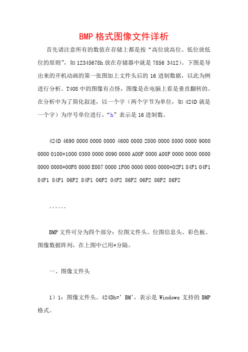
下图是导出来的开机动画的第一张图加上文件头后的16进制数据，以此为例进行分析。

T408中的图像有点怪，图像是在电脑上看是垂直翻转的。

在分析中为了简化叙述，以一个字（两个字节为单位，如424D就是一个字）为序号单位进行，“h”表示是16进制数。

424D 4690 0000 0000 0000 4600 0000 2800 0000 8000 0000 9000 0000 0100*1000 0300 0000 0090 0000 A00F 0000 A00F 0000 0000 0000 0000 0000*00F8 0000 E007 0000 1F00 0000 0000 0000*02F1 84F1 04F1 84F1 84F1 06F2 84F1 06F2 04F2 86F2 06F2 86F2 86F2．．．．．．BMP文件可分为四个部分：位图文件头、位图信息头、彩色板、图像数据阵列，在上图中已用*分隔。

一、图像文件头1）1：图像文件头。

424Dh=’BM’，表示是Windows支持的BMP 格式。

2）2-3：整个文件大小。

4690 0000，为00009046h=36934。

3）4-5：保留，必须设置为0。

4）6-7：从文件开始到位图数据之间的偏移量。

4600 0000，为00000046h=70，上面的文件头就是35字=70字节。

5）8-9：位图图信息头长度。

6）10-11：位图宽度，以像素为单位。

8000 0000，为00000080h=128。

7）12-13：位图高度，以像素为单位。

9000 0000，为00000090h=144。

8）14：位图的位面数，该值总是1。

0100，为0001h=1。

二、位图信息头9）15：每个像素的位数。

GSM信令详解

以下对信令的介绍将分两部分进行，第一部分将介绍信令的基础性知识如：SCCP，TCAP，MAP，BSSAP等；第二部分将重点介绍这些基础性知识在实际中的应用；对第一部分的很好理解是顺利掌握第二部分的有利条件，反过来对第二部分的学习也将加深我们对第一部分的了解。

第一部分：信令的原理性知识关键词：接口，信令，SCCP，TCAP，MAP，SCCP说明：由于信令部分原理性的知识很多，因此在介绍中将分重点掌握与一般了解两种图标予以标注。

没有标注部分的重要性介于两者之间。

重点掌握：Array是学习第二部分的必要条件一般了解：有助于您更深层次的掌握信令应已经掌握的知识：MTP，TUP学习后应达到的目标：能通过分析信令迅速定位故障。

第一部分第一章：SCCP在这一章中我们将讨论A：SCCP在七号信令中的位置B：MTP寻路的局限性C：SCCP的特点和功能D：SCCP的消息和原语E：SCCP的寻址与选路其中A，B是为了引出SCCP做铺垫，C，D是SCCP的具体内容，E是SCCP的实际应用。

第一节，SCCP（信令连接控制部分）在OSI中的位置以OSI七层模型的概念来看一下SCCP的位置：性是显而易见的，但是我们为什么要引入SCCP，是否是因为MTP寻路功能的局限性致使我们要引入SCCP呢？第二节，MTP 寻路的局限性在这一节中我们将讨论MTP的局限性，为引出SCCP做好准备。

MTP是电话通信网理想的信令系统，在电话应用中所有信令消息都和呼叫电路有关，消息的传输路径一般和相关的呼叫连接路径有固定的对应关系。

但是，随着通信新业务的不断发展，越来越多的网络业务需要和远端网络节点直接传送控制消息，这些消息和连接电路无关，有些甚至与呼叫无关，如GSM中移动台和HLR，VLR之间的消息传输；有些虽然与呼叫直接相关，但是消息传输路径不一定要和呼叫连接路径相同也不要求有某种确定的对应关系。

若仍然用MTP和TUP的四级结构传送上述的消息，会带来以下问题：一，MTP是根据DPC和SIO（Service Indicator--业务指示语）来选择路由并确定终端用户的，这一寻址功能具有以下的局限性：a：SPC（信令点编码）不是国际统一编码，它由信令点所在网定义。

Matlab——m_map指南（3）——实例

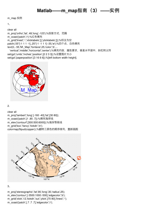
Matlab——m_map指南（3）——实例m_map 实例1、clear allm_proj('ortho','lat', 48,'long',-123');%投影⽅式，范围m_coast('patch','r');%红⾊填充m_grid('linest','-','xticklabels',[],'yticklabels',[]);%标注为空patch(.55*[-1 1 1 -1],.25*[-1 -1 1 1]-.55,'w');%四个点，⽩⾊填充text(0,-.55,'M\_Map','fontsize',25,'color','b',...'vertical','middle','horizontal','center');%填充内容，属性要求，垂直⽔平居中，斜杠转义符set(gcf,'units','inches','position',[2 2 3 3]);%设置图⽚⼤⼩set(gcf,'paperposition',[3 16 6 6]);%[left bottom width height].2.clear allm_proj('lambert','long',[-160 -40],'lat',[30 80]);m_coast('patch',[1 .85 .7]);%填充海岸线m_elev('contourf',[500:500:6000]);%海深等⾼线m_grid('box','fancy','tickdir','in');colormap(flipud(copper));%翻转三原⾊的顺序排列，重新画图3、m_proj('stereographic','lat',90,'long',30,'radius',25);m_elev('contour',[-3500:1000:-500],'edgecolor','b');m_grid('xtick',12,'tickdir','out','ytick',[70 80],'linest','-');m_coast('patch',[.7 .7 .7],'edgecolor','r');4、4.1默认的加载形式clear allSlongs=[-100 0;-75 25;-5 45; 25 145;45 100;145 295;100 290];Slats= [ 8 80;-80 8; 8 80;-80 8; 8 80;-80 0; 0 80];for l=1:7,m_proj('sinusoidal','long',Slongs(l,:),'lat',Slats(l,:));%分区块的载⼊地图m_grid;m_coast;end;xlabel('Interrupted Sinusoidal Projection of World Oceans');% In order to see all the maps we must undo the axis limits set by m_grid calls:set(gca,'xlimmode','auto','ylimmode','auto');%⾃动加载所有数据4.2clear allsubplot(211);Slongs=[-100 0;-75 25;-5 45; 25 145;45 100;145 295;100 290];Slats= [ 8 80;-80 8; 8 80;-80 8; 8 80;-80 0; 0 80];for l=1:7,m_proj('sinusoidal','long',Slongs(l,:),'lat',Slats(l,:));m_grid('fontsize',6,'xticklabels',[],'xtick',[-180:30:360],...%字体尺⼨，隐藏坐标，坐标等距离排列 'ytick',[-80:20:80],'yticklabels',[],'linest','-','color',[.9 .9 .9]);%线条形式实线，颜⾊m_coast('patch','g');%填充绿⾊end;xlabel('Interrupted Sinusoidal Projection of World Oceans');% In order to see all the maps we must undo the axis limits set by m_grid calls:set(gca,'xlimmode','auto','ylimmode','auto');subplot(212);Slongs=[-100 43;-75 20; 20 145;43 100;145 295;100 295];Slats= [ 0 90;-90 0;-90 0; 0 90;-90 0; 0 90];%⽐上⾯范围重叠更多for l=1:6,m_proj('mollweide','long',Slongs(l,:),'lat',Slats(l,:));m_grid('fontsize',6,'xticklabels',[],'xtick',[-180:30:360],...'ytick',[-80:20:80],'yticklabels',[],'linest','-','color','k');m_coast('patch',[.6 .6 .6]);end;xlabel('Interrupted Mollweide Projection of World Oceans');set(gca,'xlimmode','auto','ylimmode','auto');%⾃动加载所有数据范围5、clear all% Nice looking data[lon,lat]=meshgrid([-136:2:-114],[36:2:54]);u=sin(lat/6);%？v=sin(lon/6);m_proj('oblique','lat',[56 30],'lon',[-132 -120],'aspect',.8);%注意纬度顺序，⾼纬到低纬，'aspect'长宽⽐subplot(121);m_coast('patch',[.9 .9 .9],'edgecolor','none');m_grid('tickdir','out','yaxislocation','right',...%边缘经纬线在外，纬度在右，经度在顶'xaxislocation','top','xlabeldir','end','ticklen',.05);%边缘经纬度宽度hold on;%图层合并m_quiver(lon,lat,u,v);%经度，纬度，向东，向北的速度分量，转化为⽮量箭头xlabel('Simulated surface winds');subplot(122);m_coast('patch',[.9 .9 .9],'edgecolor','none');m_grid('tickdir','in','yticklabels',[],...'xticklabels',[],'linestyle','none','ticklen',.02);%经纬线去除hold on;[cs,h]=m_contour(lon,lat,sqrt(u.*u+v.*v));%画出轮廓clabel(cs,h,'fontsize',10,'Color','red','FontWeight','bold');%标注轮廓，字体，字体⼤⼩，颜⾊xlabel('Simulated something else');6、clear all% Plot a circular orbitlon=[-180:180];lat=atan(tan(60*pi/180)*cos((lon-30)*pi/180))*180/pi;m_proj('miller','lat',80);%查询，纬度（-80 80），经度（-180 180）m_coast('color',[0 .6 0]);m_line(lon,lat,'linewi',2,'color','r');%线宽，2；颜⾊m_grid('linestyle','none','box','fancy','tickdir','in');%没有⽹格，边框相间，%m_line(lon,lat,'linewi',2,'color','r','linestyle',':');控制线条格式，点画线还是直线7、clear allm_proj('lambert','lon',[-10 20],'lat',[33 48]);%范围设置与投影有关系m_tbase('contourf');%画5-min数据库轮廓m_grid('linestyle','none','tickdir','out','linewidth',3);没有安装terrainbase,所以轮廓很简陋，这个坑⽤到的时候再填8、不同分辨率情况下画的图clear all% Example showing the default coastline and all of the different resolutions% of GSHHS coastlines as we zoom in on a section of Prince Edward Island.clfaxes('position',[0.35 0.6 .37 .37]);%[left bottom width height]m_proj('albers equal-area','lat',[40 60],'long',[-90 -50],'rect','on');%⽅形，扇形m_coast('patch',[0 1 0]);%填充m_grid('linest','none','linewidth',2,'tickdir','out','xaxisloc','top','yaxisloc','right');m_text(-69,41,'Standard coastline','color','r','fontweight','bold');%经纬度，内容，格式axes('position',[.09 .5 .37 .37]);m_proj('albers equal-area','lat',[40 54],'long',[-80 -55],'rect','on');m_gshhs_c('patch',[.2 .8 .2]);m_grid('linest','none','linewidth',2,'tickdir','out','xaxisloc','top');m_text(-80,52.5,'GSHHS\_C (crude)','color','m','fontweight','bold','fontsize',14);axes('position',[.13 .2 .37 .37]);m_proj('albers equal-area','lat',[43 48],'long',[-67 -59],'rect','on');m_gshhs_l('patch',[.4 .6 .4]);m_grid('linest','none','linewidth',2,'tickdir','out');m_text(-66.5,43.5,'GSHHS\_L (low)','color','m','fontweight','bold','fontsize',14);axes('position',[.35 .05 .37 .37]);m_proj('albers equal-area','lat',[45.8 47.2],'long',[-64.5 -62],'rect','on');m_gshhs_i('patch',[.5 .6 .5]);m_grid('linest','none','linewidth',2,'tickdir','out','yaxisloc','right');m_text(-64.4,45.9,'GSHHS\_I (intermediate)','color','m','fontweight','bold','fontsize',14); axes('position',[.55 .23 .37 .37]);m_proj('albers equal-area','lat',[46.375 46.6],'long',[-64.2 -63.7],'rect','on');m_gshhs_h('patch',[.6 .6 .6]);m_grid('linest','none','linewidth',2,'tickdir','out','xaxisloc','top','yaxisloc','right');m_text(-64.18,46.58,'GSHHS\_H (high)','color','m','fontweight','bold','fontsize',14);运⾏出现这样问题⽹站https:///mgg/shorelines/data/gshhs/oldversions/version1.10/下载下载version1.10中 gshhs_1.10.zip ⽂件，将zip⽂件解压，把gshhs_*.b ⽂件复制到 matlab\R2009\toolbox\matlab\m_map\@private ⽂件夹内。

1、下载文档前请自行甄别文档内容的完整性，平台不提供额外的编辑、内容补充、找答案等附加服务。
2、"仅部分预览"的文档,不可在线预览部分如存在完整性等问题,可反馈申请退款(可完整预览的文档不适用该条件!)。
3、如文档侵犯您的权益，请联系客服反馈,我们会尽快为您处理(人工客服工作时间：9:00-18:30)。

M_Map：用户指南1.4版1。

入门首先，获得所有文件，无论是作为一个zip压缩包或gzip压缩的tar 文件并解压缩。

如果你解压了zip文件，请确保您还解压了子目录！现在，启动Matlab程序（版本5或更高版本）。

确保“工具箱”在您的路径。

这可以简单地通过CD ING到正确的目录。

注意：您可能要，安装M_Map所有用户访问一个工具箱。

但是，我们应该首先检查的基本设置是OK的。

第一行初始化设计。

默认值被设置为不同的投影，这样你就可以很容易地看到一个特定的投影是什么样的，但所有的设计有一些可选参数。

但是，请注意，东经指定使用有正负之分的标记法-东经是正的，而西经度是负的（还要注意，使用一个十进制度表示，这样东经120 30'W被指定为-120.5）。

第二行绘制海岸线，使用1/4度数据库。

海岸线与更高的分辨率可以使用自己的数据库（见第7节）。

m_coast 可以调用不同的线路参数。

例如，m_coast（'linewidth'，2，“color”，'r'）;m_coast（'线宽'，2，“颜色”，'r'）;画了较粗的红色海岸线。

填充的的海岸线也可以画出，使用“patch（修补）”选项（后面的任何通常的PATCH属性/值对）。

m_coast('patch',[.7 .7 .7],'edgecolor','none');m_coast（'修补'，[0.7 0.7 0.7]，'edgecolor'，'没有'）;用灰色填充和无边框绘制的海岸线。

第三条语句是叠加网格。

虽然有很多可能的选项，可用于自定义外观的网格，默认可以随时使用（在本例中）在第4节讨论这些选项。

你可以得到一个使用GET语法的选项列表：m_grid get它的作用有点像（GCA）的语法进行有规则地图形绘制。

最后，假设您想要显示和标注的位置，也就是说，一个停泊在129W，48 30'N。

[X,Y]=m_ll2xy(-129,48.5);line(X,Y,'marker','square','markersize',4,'color','r');text(X,Y,' M5','vertical','top');m_ll2xy（和它的逆m_xy2ll）用于经度/纬度坐标转换来与投影匹配。

各种裁剪选项，也可以指定在转换到投影坐标。

如果你愿意接受默认的剪切设置，您可以使用内置的功能m_line和m_text的：m_line(-129,48.5,'marker','square','markersize',4,'color','r');m_text(-129,48.5,' M5','vertical','top');最后（！），我们可能需要稍微改变网格的详细信息。

需要注意的是，在给定的地图只能被初始化一次。

clfm_coast('patch',[.7 .7 .7],'edgecolor','none');m_grid('xlabeldir','end','fontsize',10);m_line(-129,48.5,'marker','square','markersize',4,'color','r');m_text(-129,48.5,' M5','vertical','top');2。

指定预测为了得到一个列表，目前的预测，m_proj get或m_proj('set');目前返回下面的列表：Available projections are:Stereographic 立体的Orthographic 正交Azimuthal Equal-area 方位等面积Azimuthal Equidistant 方位等距Gnomonic 大圆Satellite 卫星Albers Equal-Area Conic 阿尔伯斯等面积圆锥Lambert Conformal Conic 兰伯特等角圆锥Mercator 墨卡托Miller Cylindrical 米勒圆柱Equidistant Cylindrical 等距圆柱Oblique Mercator 斜轴墨卡托Transverse Mercator 横轴墨卡托投影Sinusoidal 正弦Gall-Peters 胆-彼得斯Hammer-AitoffMollweideRobinson 罗宾逊UTM如果你想这些预测可能的选项，其名称添加到上面的命令，例如：m_proj('set','stereographic');'Stereographic'<,'lon<gitude>',center_long><,'lat<itude>', center_lat><,'rad<ius>', ( degrees | [longitude latitude] )><,'rec<tbox>', ( 'on' | 'off' )>您还可以得到关于当前投影的详细信息。

例如，为了看什么默认参数为正弦投影，我们首先对它进行初始化，然后使用“设置”选项：m_proj('sinusoidal');m_proj getCurrent mapping parameters -Projection: Sinusoidal (function: mp_tmerc)longitudes: -90 30 (centered at -30)latitudes: -65 65Rectangular border: offm_proj（'正弦'）;m_proj当前映射参数-投影：正弦（功能：mp_tmerc）的经度：-90 30 （中心在-30）纬度：-65 65矩形边框：关闭为了初始化一个projection，通常指定的某些位置参数定义的几何形状的投影（纵向限制，中央平行的，等），以及作为参数定义的范围内的地图（不管它是在一个矩形轴，边界点是什么，等等）。

这些略有不同，从投影到投影。

两个有用的属性的投影（1）能够保持角度差异小的区域（2）可以维护地区。

投影满足第一条件被称为适形，那些满足第二被称为相等的面积。

无投影二者皆可满足。

许多投影（特别是全球投影）都不满足，而不是已经试图作出美学平衡这两个条件中的错误。

注：目前，大多数投影是球形，而不是椭圆形。

UTM是一个椭圆形的投影，如果需要的话，可以指定椭圆等角圆锥投影和Albers等面积圆锥。

这有时是有用的，当你有加拿大的省或美国各州数据（例如，从一个地理信息系统软件包），这往往是使用这些投影。

这是不可能的，这将是在正常使用中的一个问题。

方位预测方位角的预测是在地球上的点被投射到一个平面的切平面。

地图使用这些预测的方向或从中心点到所有其他点的方位正确显示的属性。

大圆路线穿过中心点显示为直线（虽然大圆不穿过中央的点可能会出现弯曲）。

通常，这些地图绘制的圆形边界。

下面的参数需要定义一个方位投影：<,'lon<gitude>',center_long><,'lat<itude>', center_lat>这些参数定义了地图的中心点。

指定的经度是在地图的中心是垂直对齐的，其北端在地图的顶部（但看到下面的选项rotangle，）<,'rad<ius>', ( degrees | [longitude latitude] )>这定义地图的半径长度。

要么以度的角距离，可以给定的（例如，90为一个半球），或者可以指定的边界上的一个点的坐标。

<,'rec<tbox>', ( 'on' | 'off' | 'circle' )>默认情况下是在一个圆形边界附上地图（使用后两个选项选择），但也可以指定一个矩形。

然而，矩形地图通常是更好的使用某种形式的圆柱或圆锥投影绘制。

<,'rot<angle>', degrees CCW>这个是旋转图形以使中央的经度是不垂直的。

●Stereographic立体投影是等角的（正形投影的），但不等面积。

此投影往往用于极地区域。