A Study of the Quasi-elastic (e,e'p) Reaction on $^{12}$C, $^{56}$Fe and $^{97}$Au
高二英语哲学思想初探单选题30题

高二英语哲学思想初探单选题30题1. Philosophy is the study of _______ and the nature of reality.A. wisdomB. knowledgeC. truthD. thought答案:C。
本题主要考查哲学中对研究对象的理解。
选项A“wisdom”意为智慧;选项B“knowledge”意为知识;选项C“truth”意为真理,哲学研究的是真理和现实的本质;选项D“thought”意为思想,相比之下,“truth”更符合哲学研究的核心。
2. In philosophy, a ________ is a statement that is considered to be true without needing to be proved.A. theoryB. principleC. axiomD. concept答案:C。
“axiom”在哲学中特指无需证明即被认为正确的陈述,选项A“theory”指理论;选项B“principle”指原则;选项D“concept”指概念,均不符合题意。
3. The branch of philosophy that deals with the nature of beauty and art is called _______.A. ethicsB. aestheticsC. epistemologyD. metaphysics答案:B。
本题考查哲学分支。
选项A“ethics”是伦理学;选项C“epistemology”是认识论;选项D“metaphysics”是形而上学,而“aesthetics”指美学,与美和艺术的本质相关。
4. One of the fundamental questions in philosophy is 'What is the meaning of ______?'A. lifeB. existenceC. beingD. reality答案:A。
动态光散射分析(DLS)
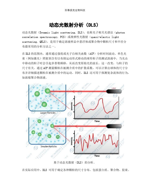
动态光散射分析(DLS)动态光散射(Dynamic light scattering, DLS),也称光子相关光谱法(photon correlation spectroscopy, PCS)或准弹性光散射(quasi-elastic light scattering, QELS),是用于确定溶液样品中悬浮体或聚合物中颗粒尺寸和半径分布最常用的分析方法之一。
在DLS的范围内,通常通过强度或光子自相关函数(ACF)分析时间波动。
单色光束(例如激光)照射到含有以布朗运动形式移动的球形粒子的测试溶液中,当光击中移动的粒子时会引起多普勒频移,从而改变原始光的波长。
这一改变,与粒子的尺寸有关。
通过ACF测量颗粒在被测介质中的扩散系数,可以计算出球体的尺寸分布并详细描述颗粒在被测介质中的运动。
同时,DLS还可用于探测复杂流体的行为,如浓缩聚合物溶液。
基于动态光散射(DLS)的分析。
在实际应用中,DLS可用于确定各种颗粒的尺寸分布,包括蛋白质、聚合物、胶束、碳水化合物和纳米颗粒。
如果系统在尺寸上不分散,则可以确定颗粒的平均有效直径,因为测量不仅取决于颗粒的核心尺寸,还取决于表面结构的尺寸、粒子浓度和介质中离子的类型。
动态光散射(DLS)分析的优点。
1. 准确、可靠和可重复的粒度分析。
2. 样品制备简单,甚至无需样品制备就可以直接对天然样品进行分析。
3. 设置简单和全自动化测定。
4. 可测量小于1nm的尺寸。
5. 可测量分子量 <1000Da的分子。
6. 体积要求低。
动态光散射DLS分析可获得重要的参数,例如分子量、回转半径、平移扩散常数等。
欢迎来电咨询!百泰派克生物科技生物制品表征服务内容。
动态光散射分析一站式服务。
您只需下单-寄送样品。
百泰派克生物科技一站式服务完成:样品处理-上机分析-数据分析-项目报告。
含沙铁路道碴弹性模量和沉降量的试验研究_季顺迎

接力 , 则依据 Mohr-Coulomb摩擦定律 , 试样与筒
体内壁间的剪切应力为 :
τ=μσr
(2)
式中 :τ为试样与筒体内壁的剪切应力 。由于对筒
体内壁进行了磨光处理 , 取碎石和细沙与光滑不锈
钢表面的摩擦因数 μ=0.15。由此 , 试样的有效法
向应力应在其名义法向应力的基础上考虑侧壁摩
擦力的影响 , 可按下式确定 :
向径向应力的传递系数 。 如果沙石混合体的内摩
擦角为 φ, 忽略其黏接力 , 则应力传递系数 k0 =1 sinφ[ 20] 。 通过动三轴试验测得道碴颗粒的内摩擦 角在 48°~ 53°之间[ 16] 。 考虑含沙铁路道碴的内摩
擦角要略低于纯道碴材料 , 这里取其内摩擦角 φ =
46°, k0 =0.28。 若试样与筒体内壁的摩擦因数为 μ, 不存在黏
-2νk0 )hu0
P A
(5)
这样 , 通过对循环加卸载过程中试样作用力 P
和位移 u的测试 , 由 (5)式即可确定含沙道碴试样
的弹性模量 。
3 含沙道碴材料的弹性模量和沉降量
采用以上试验装置和弹性模量的确定方法对 含沙道碴材料的弹性模量和沉降量进行测试 , 并在 此基础上研究细沙 -道碴混合体的力学性质随含 沙量的变化趋势 。 3.1 道碴碎石在循环加载下弹性模量和沉降量的
科技英语翻译考题整理

【科技英语翻译】考题整理1、The waster radiation is revolutionizing X-ray science, enabling researchers to see things on an atomic level with eyes that are a million times more powerful than ever before,这种被视为废物的辐射使 X 射线科学发声了一场革命:它使科研工作者能用眼睛看到原子级的东西,这一放大率比以往提高了 100 万倍。
2、If we had known the properties of the material, we should have made full use of it. 要是当时了解这种材料的特性的话,我们就会充分利用它了。
3 、Moving parts of a machine would wear much more rapidly without being oiled. 机器的运动部件如果不加油就会磨损的非常快。
4 、Cool slowly to minimize cracking. 要慢慢冷却,以最大限度的减少开裂。
5、Don`t let the stresses inside the material exceed the elastic limit, or else permanent deformation will result.不要使材料的应力超过弹性极限,否则会产生永久变形。
6 、Attention must be paid to the working temperature of the machine.应当注意机器的工作温度。
7 、Television is the transmission and reception of images of moving objects by radio waves. 电视通过无线电波发射和接受各种活动物体的图像。
ielts_academic_reading_practice_test_13_4ff0635013

IELTS Reading Passage - Population Movements And GeneticsPopulation Movements And GeneticsOrigins and distribution of human populations is studied based on archaeological and fossil evidence. From the 1950s, numerous techniques have been used which are more objective. Information about early population movements now obtained by 'archaeology of the living body', the clues are taken from the genetic material.These values of the techniques are ensured by the work on the problems which deal with when people entered America. The launching ground of human colonisers of the New World is North-east Asia and Siberia. It was found that major migration happened across the Bering Strait into the Americans. New clues have derived from the research into genetics which includes the genetic markers in modern Native Americans.Biological Anthropologist Robert Williams found one particular protein (immunoglobulin G) in the form of fluid in the blood. Most of the proteins produce variants and interbreeding human population members will share these sets of variants. One can determine their genetic distance by comparing the Gm allotypes of two different populations. This informs the length of time.In the span of a twenty year period, Williams and his colleagues collected the sample of over 5,000 American Indians in Western North America. . Gm allotypes can be divided into two groups, one of them corresponds to the genetic typing of Central And South American Indians. Apart from this, other tests showed that Aleut3 and Inuit formed a third group. It was found from the evidence that there have been three migration waves that happened across the Bering Strait. da about 600 or 700 years ago). The third wave, perhaps 10,000 or 9,000 years ago, saw the migration from North-east Asia of groups ancestral to the modern Eskimo and Aleut.To what extent does other research support these conclusions ? Douglas Wallace, a geneticist, studied mitochondrial DNA4 in the blood samples from three distinct Native American Groups: Arizona’s Pima-Papago Indians, Maya Indians on the Yucatan Peninsula, Mexico, and Ticuna Indians in Brazil's Upper region. According to the prediction of Robert Williams’s work, all three groups seem to be descended from the same ancestor - thePaleo-indian population.There are two other sorts of research which throws some light on the Native American Population origination. It involves the study of teeth and of languages. The biological anthropologist Christy Turner, having an expertise in analysing the changing physical characteristics in human teeth. According to him, tooth crowns and roots possess a high genetic component, affected by environmental and other factors in a minimal fashion. Turner studied many thousands of New and Old World Specimens, both ancient and modern and finds that most of the prehistoric Americans are connected to Northern Asian Populations byroot and crown traits such as incisor shovelling ( a scooping out on one or both surfaces of the tooth ), triple-rooted lower first molars and single-rooted upper first premolars.As stated by Turner, this ties in with the idea of a single Paleo-Indian migration out of North Asia, which he fixes before 14,000 years ago by calibrating rates of dental micro-evaluation. Analysing the tooth suggests that there were two later migrations of Eskimo-Aleut andNa-Denes.Since the 1950s, the linguist Joseph Greenberg has argued that all Native American languages belong to a single ‘Amerind’ family, Na-Dene and Eskimo-Aleut is an exception -a view that supports the idea of three main migrations. Among fellow linguists, Greenberg is a minority, who favour the idea of many waves of migration to account for the fact that American Indians speak more than 1000 languages at one time. Greenberg’s view is supported by the new genetic and dental evidence. However, dates given for the migrations should be treated cautiously, excluded where supported by hard archaeological evidence. Population Movements And Genetics IELTS Reading QuestionsQuestions 1 - 7Answer the questions below.Choose NO MORE THAN THREE WORDS from the passage for each answer.1.Where from the clues on early population movements was taken by ?2.What protein Robert Williams found in the form of fluid in the blood ?3.What could be determined by comparing the Gm allotypes of two differentpopulations ?4.How many groups are there in Gm allotypes ?5.Who studied mitochondrial DNA4 from three different Native American Groups’ bloodsamples ?6.Which study throws a light on origins of the Native American Population other thanstudy of languages ?7.Who is an expert in analysing changing physical characteristics of human teeth ?Questions 8-13Complete the summary below.Write NO MORE THAN TWO WORDS from the passage for each answer.From the8______, numerous techniques have been used which are more objective to study the fossil evidence. Information about early population movements now obtained by '9____of the living body', the clues are taken from the genetic material. Modern10________,new clues have been derived from the research into genetics which includes the genetic11______. Biological Anthropologist12_______found one particular protein (immunoglobulin G) in the form of fluid in the blood. One can determine their genetic distance by comparing the13_______of two different populations.。
朝花夕拾2-7 欧洲规范的荷载组合

欧洲规范的荷载组合(Actions and combinations of actions) Preface对于任何国家和地区的建筑结构规范体系而言,可靠度指标及其荷载规范(指荷载组合的规定)是整个规范体系的“总纲”,要想全面了解该规范体系,须首先研究其荷载规范,这正是我做此读书笔记之原因。
欧洲的规范的可靠度也是采用半系数(半概率极限状态)来描述,即partial factor。
本文所指的“欧洲规范”均指BS EN,即欧洲规范的英国版本。
所谓的“欧洲规范”实际不存在,它只是一个范本,在各个国家都有具体的本地化欧洲规范,方法和公式是统一的,各国可能会用不同的系数,还会增加一些附录。
为展现规范原貌,读书笔记都直接摘录英语原文,不作翻译。
感觉欧洲规范体系严谨,但条文繁琐(相比英国规范和美国规范)。
Index1. Introduction (2)1.1 Serviceability Limit States (2)1.2 Ultimate Limit States (2)2. Situations and Actions (3)3. Fundamental combinations of actions (4)3.1 Values of ψ factors (4)3.2 Serviceability Limit States (4)3.2.1 General (4)3.2.2 Combinations (5)3.3 Ultimate Limit States (6)3.3.1 General (6)3.3.2 Combinations – main method (6)3.3.3 Combinations – simplified method (7)3.4 For Non-Linear Analysis (7)3.5 Application for Buildings (8)3.5.1 Combination Table - Ultimate Limit States (8)3.5.2 Combination Table - Serviceability Limit States (11)3.6 Examples (11)4. Deflection in serviceability limit states (14)4.1 Vertical deflection (14)4.1.1 Definition (14)4.1.2 Limit (15)4.2 Horizontal deflection (15)4.2.1 Definition (15)4.2.2 Limit (16)5. Discussion (16)欧洲规范的荷载组合(Actions and combinations of actions) 1. IntroductionThe basis requirement of EN 1990 state that a structure shall have adequate structural resistance (ultimate limit states), serviceability (serviceability limit states), durability, fire resistance and robustness.1.1 Serviceability Limit StatesFor serviceability limit states, which are defined in clause 3.4 of EN 1990 as those that concern:The functionality of the structure or structural members under normal use.The comfort of the people.The appearance of the structure.For buildings, the primary concerns are horizontal and vertical deflections and vibrations. Three categories of combinations of loads (actions) are specified in EN 1990 for serviceability checks: characteristic, frequent and quasi-permanent.1.2 Ultimate Limit StatesFor ultimate limit states, checks should be carried out for the following, as relevant:EQU – loss of static equilibrium of the structure or any part of the structure.STR –internal failure or excessive deformation of the structure or structural members.GEO –failure or excessive deformation of the ground.FAT –fatigue failure of the structure or structural members.欧洲规范的荷载组合(Actions and combinations of actions)2. Situations and ActionsIn EuroCodes, design situations for limit states are classified as follows:Persistent design situations, which refer to conditions of normal use.Transient situations, which refer to temporary conditions, such as during execution or repair.Accidental design situations, which refer to exceptional conditions such as fire, explosion or impact.Seismic design situation, which refer to conditions where the structure is subjected to seismic events.Actions are classified as follows:(1) By their variation in time:Permanent actions (G), (e.g. dead loads such as self-weight. Fittings etc.).Variable actions (Q), (e.g. live loads including imposed floor loads, wind loads and snow loads).Accidental actions (A), (e.g. hazards such as explosions, vehicular impact and fire).(2) By their variation in space:Fixed actions (e.g. self-weight).Free actions (e.g. wind, snow and moveable imposed loads).Types of action:G – permanent actions;Q – variable actions;A – accidental actions.欧洲规范的荷载组合(Actions and combinations of actions)3. Fundamental combinations of actions3.1 Values of ψ factorsValues of ψ factors should be specified, see blow copied from table A1.1 of EN 1990.3.2 Serviceability Limit States3.2.1 GeneralAccording to clause 3.4 of EN 1990, a distinction should be made between reversible and irreversible serviceability limit states. Reversible serviceability limit states are those that would be infringed on a non-permanent basis, such as excessive vibration or high elastic deflections under temporary (variable) loading. Irreversible serviceability limit states are those that would remain infringed even when the cause欧洲规范的荷载组合(Actions and combinations of actions)of infringement was removed (e.g. permanent local damage or deformations).3.2.2 CombinationsThree categories of combinations of loads (actions) are specified in EN 1990 for serviceability checks: characteristic, frequent and quasi-permanent.1, characteristic combination:(6.14a of EN1990)E E G , ;P;Q , ;ψ , ,Q , j 1;i iIn which the combinations of actions in brackets { } (called the characteristic combination), can be expressed as(6.14b of EN1990) :G , P Q , ψ ,Q ,Note: the characteristic combination is normally used for irreversible limit states.2, frequent combination:(6.15a of EN1990)E E G , ;P;ψ , ,Q , ;ψ , ,Q , j 1;i iIn which the combinations of actions in brackets { } (called the frequent combination), can be expressed as(6.15b of EN1990):G , P ψ , Q , ψ ,Q ,Note: the frequent combination is normally used for reversible limit states.3, quasi-permanent combination:(6.16a of EN1990)E E G , ;P;ψ , ,Q , j 1;i iIn which the combinations of actions in brackets { } (called the quasi-permanent combination), can be expressed as(6.16b of EN1990):G , P ψ ,Q ,Note: the quasi-permanent combination is normally used for long-term effects and the appearance of the structure.For serviceability limit states the partial factors for actions should be taken as 1.0 except if differently specified in EN 1991 to EN 1999. Check Annex A1 of EN 1990 for欧洲规范的荷载组合(Actions and combinations of actions) detailing of combinations, which is also a appendix of this article.3.3 Ultimate Limit States3.3.1 General“Fundamental” refers to the persistent or transient design situations, rather than accidental or seismic design situations. There are two options for the fundamental combination of actions at ultimate limit states: main method and s implified method.3.3.2 Combinations – main method1, (Fundamental Combinations) Combinations of actions for persistent or transient design situations:(6.10 - EN 1990)γG, G , γ P γQ, Q K, γQ,ψ , Q ,Or, alternatively for STR and GEO limit states, by less favorable of the two following expressions:(6.10a - EN 1990)γG, G , γ P γQ, ψ , Q K, γQ,ψ , Q ,(6.10b - EN 1990)ξ γG, G k,j γ P γQ, Q K, γQ,ψ , Q ,ψ0:combination factorξ: reduction factor for unfavorable permanent actions G.γG: partial factor for permanent actions.γQ: partial factor variable actions.P: represent actions due to prestressing.2, Combinations of actions for accidental design situations: (6.11b - EN 1990)G k,j P A ψ , or ψ , Q K, ψ , Q ,A d: accidental actionNotes:(1) The choices between ψ1,1Q k,1 or ψ2,1Q k,1 should be related to the relevant欧洲规范的荷载组合(Actions and combinations of actions)accidental design situation (impact, fire or survival after the accidental event or situation).(2) Combinations of actions for accidental design situations should either- involve an explicit accidental action A (fire or impact), or-refer to a situation after an accidental event (A=0).3, Combinations of actions for seismic design situations:(6.12b - EN 1990)G k,j P A E ψ , Q ,A Ed: seismic action3.3.3 Combinations – simplified methodThe second method is a simplified alternative for building structures, which calls for two checks as examples in 3.6, see below. The first check combines one variableaction at a time along with the permanent actions, using the standard value of γQ..The second check combines all variable actions at one time with the permanent actions, using a reduced value 0.9γQ.Note: I find this method in <<Interim Guidance on the use of Eurocode 3: Part 1.1 for European Design of Steel Building Structures>>, but I can’t find similar clauses in the formal Guidance and BS EN 1990.3.4 For Non-Linear AnalysisFor non-linear analysis (i.e. when the relationship between actions and their effects is not linear), expressions (6.9a) or (6.9b) should be applied directly, depending upon the relative increase of effects of actions compared to the increase in the magnitude of actions. The following simplified rules may be considered in the case of a single predominant action :a) When the action effect increases more than the action, the partial factor γF shouldbe applied to the representative value of the action.b) When the action effect increases less than the action, the partial factor γF shouldbe applied to the action effect of the representative value of the action.欧洲规范的荷载组合(Actions and combinations of actions) NOTE: Except for rope, cable and membrane structures, most structures or structural elements are in category a).3.5 Application for BuildingsMethods for establishing combinations of actions for buildings are given in Annex A1 of EN 1990. The combination guidance tables are copied as follow.3.5.1 Combination Table - Ultimate Limit States欧洲规范的荷载组合(Actions and combinations of actions)欧洲规范的荷载组合(Actions and combinations of actions)To simplify building design, note 1 to clause A1.2.1(1) of EN 1990 allows the combination of actions to be based on not more than two variable actions. This simplification is intended to only to apply common cases of building structures. The following is clause of Note 1: Depending on its uses and the form and the location of a building, the combinations of actions may be based on not more than two variable actions.欧洲规范的荷载组合(Actions and combinations of actions) 3.5.2 Combination Table - Serviceability Limit States3.6 ExamplesExamples from the interim guidance:欧洲规范的荷载组合(Actions and combinations of actions)Examples from the formal guidance:欧洲规范的荷载组合(Actions and combinations of actions)欧洲规范的荷载组合(Actions and combinations of actions)4. Deflection in serviceability limit states4.1 Vertical deflection4.1.1 Definition欧洲规范的荷载组合(Actions and combinations of actions) 4.1.2 Limit4.2 Horizontal deflection4.2.1 Definition欧洲规范的荷载组合(Actions and combinations of actions) 4.2.2 LimitNote: All the clauses in section 4 are just for EN 1993-1.5. Discussion1)可能是由于欧洲处于新旧规范更替时代,我发现许多(senior)欧洲结构工程师对欧洲规范条文也是一知半解。
prony series finite element
PRONY SERIES FITTING METHOD TO CREEP EXPERIMENTAL DATA WITHDIFFERENT NUMBERS OF ELEMENTSLucas Feitosa de A. L. BabadopulosDidier BodinEmmanuel ChailleuxSylvia DreessenCentre de Recherche de Solaize de TOTAL - CReSLaboratoire Central des Ponts et Chaussées - LCPCLaboratoire Central des Ponts et Chaussées – LCPCCentre de Recherche de Solaize de TOTAL - CReSRESUMOEste trabalho descreve um método de ajuste de séries de Prony sobre dados de fluência. Foi utilizado o reômetro Bending Beam Rheometer (BBR). Um modelo de Kelvin-Voigt Generalizado (de graus de liberdade D j and τj) foi utilizado para se obter séries de Prony. Foi variado o numero de elementos neste estudo da precisão de ajuste através da função Custo residual (diferenças quadradas entre previsão do modelo e dados experimentais para cada ponto experimental). As constantes temporais são pré-selecionadas em uma escala logarítmica baseada no domínio temporal dos dados. O método foi implementado em Scilab. A utilização de um número maior de constantes não melhora sempre a acurácia do ajuste, mas tende a aumentar a probabilidade de um bom ajuste (o comportamento mecânico de materiais viscoelásticos lineares pode, teoricamente, ser representado por séries de Prony infinitas). A função custo residual evolui com o número de tempos de relaxação do modelo apresentando a tendência de decrescer periodicamente.ABSTRACTThis paper describes a method to fit Prony series to creep experimental data. The test used is the Bending Beam Rheometer (BBR). A Generalized Kelvin-Voigt model (degrees of freedom D j and τj) was used to obtain the Prony series. Different numbers of elements were used to study the fitting accuracy by the means of the residual cost function (squared differences between model prediction and experimental data for each data point). The time constants were preselected in a logarithmic scale based on the experimental time domain. A Quasi-Newton optimization algorithm was used to determine the set of Dj minimizing the residual function. The method was implemented in Scilab. Using bigger number of elements does not always increase the accuracy of a fitting but it possibly increases the probability of a good fitting (theoretically a linear viscoelastic material can be represented by a Kelvin-Voigt Model with an infinity of elements). The residual cost function decreases periodically with the requested number of relaxation times for the model.1. INTRODUCTIONAsphalt provides to the asphalt mixes used in road infrastructure their viscoelastic properties. It is useful to estimate the mechanical response evolution of these materials while they are currently used. In viscoelasticity, for different load histories the materials present different strain evolution in the time domain. Frequently, in order to estimate the relation between stress and strain evolution in asphalt materials, the linear viscoelasticity theory is applied. Obtaining experimental data relating stress and strain allows us to represent this relation by means of mathematical functions. These functions are obtained by fitting mechanical models response to experimental data. The most used models are the Generalized Kelvin-Voigt and the Generalized Maxwell Model, both resulting in modeled mechanical responses mathematically described by Prony series. Many authors describe fitting procedures using this kind of series (Schapery 1961; Sousa and Soares 2008). Linear Viscoelastic properties like Complex Modulus or Creep Compliance are meant to be intrinsic and interconversible properties for each material, in a way that the knowledge of one of them allows us to obtain the other (Park and Schapery 1999; Silva et al. 2008). In this paper, only a curve fitting method of Prony series to creep data is presented.2. CREEPThis phenomenon is defined as the continuous increasing deformation occurring in a material under constant loading. It is very sensible to time variations. Different tests allow us to access creep information, in different loading modes (traction, compression, bending,...). For this work, only the Bending Beam Rheometer was used, which is a three points flexural test.2.1. Bending Beam Rheometer (BBR)In this study, the Bending Beam Rheometer (BBR) was used to access creep data. It provides a measure for low-temperature creep tests. Asphalt beams are prepared in an aluminum mold. Storage time for each sample was 24 hours. After one hour at the test temperature, a constant load of 100 g was applied for 240 seconds to the rectangular beam supported at both ends by stainless steel half-rounds (set 102 mm apart). Center-point deflection is measured continuously. By using a linear interpolation, these tests give a measure of creep stiffness at any moment and any temperature (AASHTO T313-02). An ethanol bath controls the test temperature.Its principle is to measure the deflection in the center-point of a bitumen beam at low temperature (-36 to 0°C, for this work we performed tests above -24°C) in three points bending (Figure 1).Figure 1: Measured deflection and imposed force in a BBR creep testThe viscoelastic property output through this test is the Secant Modulus S(t): )(.4)()()(33t bh PL t t t S δεσ== (1)For a constant load this property is directed related to the Creep Compliance J(t) as simply the inverse:)(1)(.)()()(t J t J t t t S ===σσεσ(2)2.2. Time-temperature superposition principleIn order to obtain the Creep Compliance in time tests not accessible by the experiments, the time-temperature superposition principle is used. This principle states that an increase in the time of loading leads to the same effects in the material as an increase in the temperature. This considers that the material internal structure does not change with the temperature changing. This principle is currently applied to most part of the asphalts used nowadays producing good results. A mathematical form of this principle is:),(),(),(2211i i t T J t T J t T J ==(3) )),(,(),(0i i i i t T T J t T J α=(4) where T: test temperature in KelvinT 0: reference temperature in Kα (T i ,t i ): transposition function for which the form is a T (T i ).t i .2.3. Master curves for creep complianceUsing the time-temperature superposition principle, we get from the data presented in Figure 2 to the Master Curve presented in Figure 3 using different methods (Arrhenius Law, William Landels Ferry Law or a simple manual transposition as first approximation).Figure 2: Example of experimental Creep Compliance at different temperaturesMaster Curve at -10°C-4-3-2-10123log(t)J (t ) (1/M p a )Figure 3: Example of a Master Curve for Creep Compliance at -10°C as referencetemperature3. USED MATERIALS: ASPHALT BINDERSThis study used eight asphalts selected according to the origin of the crude petroleum, manufacturing process, and type of modifiers used. Three direct-distilled asphalts of different origins (B 1, B 2 and B 3) and one semi-blown asphalt (B 4) with the same 35/50 penetration (standard NF EN 12591) were used. Four types of adjuvant were used to modify the B 1 asphalt: Sasobit ® paraffin wax (B M1), polyphosphoric acid at 105-118% (B M2), crosslinker-free SBS polymer (B M3) and crosslinked SBS polymer (B M4).4. THE KELVIN-VOIGT MODEL (KVM)4.1. Simple KVMThis model consists in the parallel association of a spring (εσE =, E is the constant stiffness)and a dashpot (εησ&=, η is the constant of viscosity). Figure4 presents the model and defines the relaxation time τ.Figure 4: Simple Kelvin-Voigt ModelKnowing its mechanical solution under constant stress ()1()(/τσεt e E t −−=) the Creep Compliance can be calculated:)1()1(1)1()()(///τττσσσεt t t e D e E e E t t J −−−−=−=−== (5)4.2. Generalized KVMThe Generalized KVM consists in the series association of a perfectly rigid element withmany Kelvin-Voigt elements.Figure 5: Generalized Kelvin-Voigt ModelUsing Equation 5 we deduce the expression for the Creep Compliance of this model summing the response of each element under constant stress: ∑∑∑=−=−=−−+=−+=−+==n j t j g n j t j n j t j j j j e D D e E E e E E t t J 1/1/01/0)1()1(11)1()()(τττσσσσε (6)where D j and τj can be seen as the degrees of freedom of the Prony series that represents J(t).D g is the Compliance in the glassy state.5. FITTING PROCEDUREThe fitting procedure presented here was implemented in Scilab. It consists in the steps described above:• Preselection of the vector containing the relaxation times τj in a logarithmic scale.o The first relaxation time is the first decade contained in the experimental timedata vector.o The last relaxation time is the decade immediately after the last decade in theexperimental time data vector.o The other relaxation times are distributed logarithmically between the first andthe last one. By this technique, we can vary the number of elements of theKVM and evaluate each fitting of the model to the data.• Determination of the elastic element’s constant. It is directly inferred from theminimum experimental value of Creep Compliance J (Sousa and Soares 2007).• Setting of the initial guess of the Prony series. A purely elastic KVM with the sameelastic element D g as the experimental data was chosen.• Definition of the cost function (square difference between model prediction andexperimental data) and its derivative (calculated by a Scilab function).• Definition of the bounds for D j (the elements cannot be negative).• Optimization of the residual function f and calculation of the parameters of the model.A Quasi-Newton optimization algorithm (only one in Scilab accepting bounds) is used. The residual cost for the optimal set of D j f(xopt) is taken as fitting accuracy indicator.A numerical example is shown in Figure 6 to validate this procedure. A simulated creep compliance was generated from a set of five arbitrary Kelvin Voigt elements D j and τj . The figure shows the number of elements used and the residual cost f(xopt) for the fitted model in parentheses.In Figure 7 an evaluation of the number of elements’ influence over the residual cost function is presented for the numerical simulation. Of course, the minimum value of this function was obtained for the optimization with five elements (simulated material’s original number of elements).Figure 6: Numerical validation of the KVM parameters identification procedureFigure 7: Evaluation of the number of elements’ influence in the Residual cost function forthe simulated material6. RESULTS AND DISCUSSIONFor different number of parameters, different fitted models were obtained. Figure 8 shows sixteen different fittings (using from 1 to 16 Kelvin-Voigt elements) to creep compliance data obtained at -5°C for the reference asphalt binder. This is an example of the general tendency of periodic well calibrated models which occurred for each asphalt binder studied in this paper (even the simulated material).Figure 8: Curve fittings for the reference asphalt binder (Master curve at -5°C) These figures show that higher numbers of requested elements do not always improve the curve fitting. Generally, the decrease in the fitting accuracy is associated with KV elements which assumed zero rigidity during the optimization process. Figure 9 shows the KV elements obtained for the fittings with six and seven relaxation times (requested by the algorithm) to the reference asphalt binder experimental data. Both sets of KV elements have the same purely elastic element (76.7 MPa-1). We can see that when seven elements were requested only four were obtained (three of the seven elements assumed zero rigidity). This may occur because some of the selected relaxation times are not compatible with the actual material’s relaxation spectra.Figure 9: Viscoelastic KV elements obtained for a set of six and seven preselected relaxationtimesAs it was done for the simulated material, Figure 10 shows the evolution of the residual cost function with the number of Kelvin-Voigt elements used in the calibration method.Figure 10: Residual cost function vs Number of elements of the Prony series for B17. CONCLUSIONWith the procedure described in this paper we could fit Prony series to creep compliance data. Different fittings were performed varying the number of elements of the Prony series. Based on the data shown in this paper, it can be said that the evolution of the residual cost function is not monotonic, but it shows a periodic decreasing tendency for all asphalt binders. This is in agree with the theoretical equivalence between infinite Prony series and linear viscoelastic materials’ mechanical behavior. Between one and sixteen parameters a comparison between the fittings is suggested to choose the number of elements in order to obtain a better fitting accuracy. This procedure allows the identification of Prony series describing linear viscoelastic properties based on creep data.AcknowledgementsThe authors would like to thank the French company Total and the LCPC for their researching support and cooperation.REFERENCESFerry, J. D. (1980) Viscoelastic Properties of Polymers. 3e ed. John Wiley and Sons, New York. Hammoum, F.; Chailleux, E.; Nguyen, H-N. ; Erhlacher, A.; Piau, J-M ; Bodin, D. (2009) Experimental and Numerical Analysis of Crack Initiation and Growth in Thin Film. Road Materials and Pavement Design.EATA, P 39-61.Park S. W. and Schapery R. A. (1999) Methods of interconvertion between liner viscoelastic material functions.Part I – a numerical method based on Prony series. International Journal of Solids and Structures, vol.36, p. 1653-1675.Schapery R. A. (1961) A simple collocationg method for fitting viscoelastic models to experimental data.Rep.GALCIT SM 61-23A, California Institute of Technology, Pasadena, USA.Silva, H. N.; Sousa, P. C.; De Holanda, A. S.; Soares, J. B. A (2008) Computer program for linear viscoelastic characterization using Prony Series. XXIX CILAMCE - Iberian Latin American Congress on Computational Methods in Engineering. Maceio, Brésil.Sousa, P. C.; Soares, J. B. (2007) Método da colocação para obtenção de séries de Prony usadas na caracterização viscoélastica de materiais asfalticos. XXI Congresso de Pesquisa e Ensino em Tranportes – ANPET. Rio de Janeiro, Brésil.Williams, M. L.; Landel, R. F.; Ferry, J. D. (1955) The temperature dependence relaxation mechanism in amorphous polymers and other glass forming liquids. Journal of ACS, vol. 77, pp 3701.。
广东工业大学物理学院导师简介

物理学院导师简介硕士教育材料物理与化学(硕士)学科、专业培养目标:具有坚实的材料物理与化学理论基础和系统的专门知识。
了解本学科的发展动向。
掌握材料结构及其物理性质和化学性质研究的基本方法和技术。
熟练掌握运用一门外国语和计算机。
有较强的知识更新能力和熟练的实验技能,掌握有关先进的材料制备技术和先进测试仪器的使用和结果分析。
具有在材料或器件的研究开发单位、高等院校或生产部门工作的能力。
主要课程: 量子力学(Ⅱ)、固体物理(Ⅱ)、高等激光技术、纳米材料与纳米技术、群论、固态电子学、激光光谱学、半导体薄膜技术、新型复合材料理论与应用、光信息存储材料、光电材料及器件物理、计算物理、材料科学前沿、激光与物质相互作用、材料化学、Matlab在工程中的应用、X射线衍射与电子显微分析。
物理电子学(硕士)学科、专业培养目标:物理电子学是近代物理学、电子学、光学、光电子学、量子电子学及相关技术的交叉学科,主要在电子工程和信息科学技术领域内进行基础和应用研究。
硕士生通过三年左右时间的学习学生应具有较坚实的数学、物理基础知识,常据本学科坚实的理论基础及系统的专门知识;掌据相关的实验技术及计算机技术。
较为熟练地掌据一门外国语,能阅读本专业的外文资料。
具有从事科学研究工作及独立从事专门技术工作的能力,以及严谨求实的科学态度和工作作风;能胜任研究机构、高等院校和产业部门有关方面儒教学、研究、工程、开发及管理工作。
主要课程: 光电子学与激光器件、微电子器件原理与应用、固体物理学Ⅱ、激光光谱学、量子力学、薄膜物理技术、声学基础、物质结构、Matlab在工程中的应用、半导体物理学、光通信技术与器件、计算物理学、物理电子技术实验等教授,博士,硕士生导师。
1964年3月出生,2001年在中国科学技术大学获博士学位,2002-2004年中国科学院固体物理研究所博士后。
现任物理学教授,硕士生导师,广东工业大学物理与光电工程学院副院长。
主讲的本科教学课程有《大学物理学》,《电子科学与技术专业导论》,《固体物理学》,《材料物理导论》,《半导体物理学》,《近代物理实验》;为研究生讲授《结构分析》,《纳米材料合成方法》,《材料物理科学前沿》等课程。
- 1、下载文档前请自行甄别文档内容的完整性,平台不提供额外的编辑、内容补充、找答案等附加服务。
- 2、"仅部分预览"的文档,不可在线预览部分如存在完整性等问题,可反馈申请退款(可完整预览的文档不适用该条件!)。
- 3、如文档侵犯您的权益,请联系客服反馈,我们会尽快为您处理(人工客服工作时间:9:00-18:30)。
a r X i v :n u c l -e x /0303011v 1 24 M a r 2003A Study of the Quasi-elastic (e,e’p)Reaction on12C,56Fe and97Au.D.Dutta 15,10,a ,D.van Westrum 4,b ,D.Abbott 22,A.Ahmidouch 7,Ts.A.Amatuoni 25,C.Armstrong 24,c ,J.Arrington 2,d ,K.A.Assamagan 6,e ,K.Bailey 1,O.K.Baker 22,6,S.Barrow 18,K.Beard 6,D.Beatty 18,c ,S.Beedoe 14,E.Beise 11,E.Belz 4,C.Bochna 9,P.E.Bosted 12,H.Breuer 11,E.E.W.Bruins 10,R.Carlini 22,J.Cha 6,f ,N.Chant 11,C.Cothran 23,W.J.Cummings 1,S.Danagoulian 14,D.Day 23,D.DeSchepper 10,J.-E.Ducret 21,F.Duncan 11,g ,J.Dunne 22,f ,T.Eden 6,R.Ent 22,H.T.Fortune 18,V.Frolov 19,h ,D.F.Geesaman 1,H.Gao 9,10,a ,R.Gilman 22,20,P.Gu`e ye 6,J.O.Hansen 1,c ,W.Hinton 6,c ,R.J.Holt 9,C.Jackson 14,H.E.Jackson 1,C.Jones 1,S.Kaufman 1,J.J.Kelly 11,C.Keppel 22,6,M.Khandaker 13,W.Kim 8,E.Kinney 4,A.Klein 17,D.Koltenuk 18,i ,L.Kramer 10,j ,W.Lorenzon 18,k ,A.Lung 2,c ,K.McFarlane 13,l ,D.J.Mack 22,R.Madey 6,7,P.Markowitz 5,J.Martin 10,A.Mateos 10,D.Meekins 22,c ,ler 9,ner 10,J.Mitchell 22,R.Mohring 11,H.Mkrtchyan 25,A.M.Nathan 9,G.Niculescu 6,m ,I.Niculescu 6,n ,T.G.O’Neill 1,D.Potterveld 1,J.W.Price 19,o ,J.Reinhold 1,j ,C.Salgado 13,J.P.Schiffer 1,R.E.Segel 15,P.Stoler 19,R.Suleiman 7,p ,V.Tadevosyan 25,L.Tang 22,6,B.Terburg 9,q ,Pat Welch 16,C.Williamson 10,S.Wood 22,C.Yan 22,Jae-Choon Yang 22J.Yu 18,B.Zeidman 1,W.Zhao 10,and B.Zihlmann 23.1Argonne National Laboratory,Argonne IL 604393Chungnam National University,Taejon 305-764Korea5Florida International University,University Park,FL 331997Kent State University,Kent OH 442429University of Illinois,Champaign-Urbana IL 6180111University of Maryland,College Park MD 2074213Norfolk State University,Norfolk VA 2350415Northwestern University,Evanston IL 6020117Old Dominion University,Norfolk,VA 2352919Rensselaer Polytechnic Institute,Troy NY 1218021CE Saclay,Gif-sur-Yvette France23University of Virginia,Charlottesville VA 2290125Yerevan Physics Institute,Yerevan,Armeniaa Present address:Duke University,Durham,NC 27708bPresent address:Micro-g Solutions Inc.,Erie,CO 805162 INTRODUCTIONThe value of studying electronuclear reactions has longbeen recognized.In such studies the entire nucleus is ac-cessed via a well-understood interaction.A new avenueof investigations has been opened up with the completionof the continuous beam,multi-GeV electron acceleratorat the Thomas Jefferson National Accelerator Facility,also known as Jefferson Lab(JLab).The present pa-per reports results from thefirst experiment done at thisfacility,which is a study of(e,e’p)reactions in the quasi-elastic region.This experiment utilized one of the ad-vantages of electron scattering,namely,the transferredenergy and momentum can be varied separately,and oneof the main features of JLab,namely,the high inten-sity continuous electron beam of CEBAF which makes itpossible to do coincidence measurements orders of mag-nitude more extensive than could be done previously.The simplest model of a nucleus is one of independentnucleons populating the lowest available shell-model or-bits.In a simple picture of e−p scattering within a nu-cleus,the electron scatters from a single protons which ismoving due to its Fermi momentum.The struck protonmay then interact with the residual A-1nucleons beforeleaving the nucleus.Of course,neither the nucleus northe scattering process are this simple and the deviationsfrom these simple pictures reveal much about nuclei andtheir constituents,both real and virtual.The presentexperiment consisted of measuring proton spectra in co-incidence with inelastically scattered electrons with theenergy of the electrons chosen such as to be in the”quasi-elastic”region,i.e.at energies corresponding to scatter-ing from single off-mass-shell nucleons.The spectra weretaken in an angular region about the”conjugate”angle,i.e.the angle for scattering from stationary nucleons,over an angular range sufficient to cover the smearing ofthe two-body kinematics caused by the Fermi momentumof the confined protons.Data were taken over the range0.64<Q2<3.25(GeV/c)2where Q2is the square ofthe four-momentum transferred to the struck proton.dΩ= dσ| q|2[G2E(Q2)+τǫ−1G2M(Q2)](3)where dσ1+2(1+τ)tan2(θQ2−1,G E is the proton electric form factor andG M is the proton magnetic form factor in units of the nuclear magneton,e3 PWIA the coincidence(e,e’p)cross sections can be writ-ten:d6σ2+tan2(θ2)]1/2W LT(q,ω)cos(φ)+λ22(1M2)(5)One can accurately determine∆E recoil because oncethedispersion has been accurately measured the only un-known in Eq.5is the beam energy E.This procedure wasrepeated for several values of the spectrometer magneticfield.With both targets a small correction was made forthe energy loss of the electrons in the target.The other method is to determine the angle of thediffraction minimum for scattering to a state where theposition can be accurately calculated.The minimum forscattering to the12Cfirst excited state has been deter-mined to be at Q2=0.129±0.0006(GeV/c)2[8].The(four)momentum transfer can be written:Q2=4EE′sin2θ1+2E sin2θM(6)where M is the mass of the scattering nucleus andθis theelectron scattering angle.An improvement in accuracyin the measurement of Q is obtained by using the ratioof elastic scattering to inelastic scattering.Again,then,the only unknown is the incident electron energy E.Thetwo methods agreed to1part in2000and the absoluteenergy determination using these methods is believed tobe accurate to10−3.These methods become less feasibleas the energy is increased.The beam energy can alsobe determined by measuring the energy and angle of thescattered particles in electron-proton elastic scattering.Because of the uncertainties in the angle and momentummeasurements this method is less accurate than the othertwo but has the advantage that it can be used over theentire range of incident electron energies.Elastic e−pscattering was used to measure the energy of the three-pass beam with an uncertainty of1part in500.Beamenergy was also determined by measuring the magneticfield needed to bend the beam around the Hall C arc.The energy calibration as well as other aspects of theexperiment are discussed more completely elsewhere[9].Beam currents of10to60µAmps were used.The cur-rents were monitored by3microwave cavities that wereinstalled for this purpose in the Hall C beam line[10].The absolute calibration was performed by comparisonwith an Unser cavity,which is a parametric DC currenttransformer with very stable gain but a drifting offsetwhich was determined as part of our daily calibrationprocedure.The overall accuracy in the beam currentmeasurement was±1%.4TargetsData were taken with≈200mg/cm2C,Fe and Au targets mounted on a steel ladder in an aluminum scat-tering chamber.The target thicknesses were determined to about0.1%.The e−p elastic scattering data used for calibration were taken using the4.0cm cell of the Hall C cryogenic target[11].During the early part of the experiment,before the cryogenic target was avail-able,some data were taken with a solid CH2target but these data were used to check some kinematic offsets only. The compositions of hydrocarbon targets are subject to change under beam irradiation and therefore all the cal-ibration data were taken with the liquid hydrogen tar-get.The cryogenic targets are also mounted on a ladder with both ladders contained in the aluminum scattering chamber.The123.0cm diameter scattering chamber has entrance and exit snouts for the beam and several pump-ing and viewing ports.The particles that went to the High Momentum Spectrometer(HMS)spectrometer ex-ited through a0.4mm aluminum window and those to the Short Orbit Spectrometer(SOS)through a0.2mm aluminum window.For both spectrometers the particles had to pass through about15cm of air before entering the spectrometer.SpectrometersData were taken with the HMS and the SOS in coinci-dence.This experiment served as the commissioning ex-periment for these spectrometers.The HMS detected the electrons and the SOS the protons,except at the highest Q2where the roles of the spectrometers were reversed.High Momentum SpectrometerThe HMS is a25o vertical bend spectrometer made up of superconducting magnets in a QQQD configura-tion.The dipolefield is monitored and regulated with an NMR probe and kept constant at the10−4level.The spectrometer rotates on a pair of rails between12.5o and 90o with respect to the beam line.The HMS maximum central momentum is7.3GeV/c and in preparing for the present experiment the spectrometer was tested up to 4.4GeV/c although the highest setting at which data were taken was2.6GeV/c.The usable momentum bite is of the spectrometer is≈20%.A momentum resolution (σ)of<1.410−3,and an in-plane(out-of-plane)angular resolution of0.8(1.0)mrad was achieved for the HMS. With no collimator in place the solid angle subtended for a point target is8.1msr.A6.35cm thick HEAVYMET (machinable Tungsten alloy,10%Cu Ni;density=17 g/cm3)collimator with aflared octagonal aperture lim-ited the solid angle to6.8msr.The higher momentum particles were usually detected in the HMS and except at the backward(electron)angles these were the electrons. Detailed information about the HMS can be found in[12].Short Orbit SpectrometerThe SOS consists of3(normal conducting)magnets in a QD5the readout interval.In the SOS chambers one pair is in the x plane and the other two pairs of planes are at±60o with respect to the x plane.Position resolution per plane is<250µm in the HMS chambers and<200µm in the SOS.The wire chamber data was used to reconstruct the trajectory of the particles and determine the particles momentum fraction relative to the central momentum,δp/p.Wire chamber tracking efficiency is an important ele-ment in the overall system efficiency and,as such,must be accurately measured.This was done by using the posi-tion information in the hodoscopes to tag particles pass-ing through a small central region of the chambers and then see what fraction of such events was reconstructed from the wire chamber signals.In both spectrometers typical tracking efficiency was greater than97%which was determined to better than1%.The main sources of wire chamber tracking inefficiency are inefficiencies in the chambers themselves(we require5of the6planes have good hits)and inefficiency in the reconstruction al-gorithm.The measured inefficiency was the sum of these inefficiencies and no attempt was made to disentangle the two.CalibrationsSpectrometer optimizationsBecause this was thefirst experiment performed in Hall C,considerable effort went intofirst optimizing the per-formance of the spectrometers and then optimizing the data analysis so as to achieve the highest possible ac-curacy.The magneticfield of the HMS quadrupoles was mapped to determine its optical axis and its effectivefield length versus current,with effectivefield length defined as the line integral of thefield divided by the average field.However,the HMS dipole was not mapped and its magneticfield to current(B-to-I)relation was cal-culated using the TOSCA program[14].The measured field map of the quadrupole and the TOSCA generated map of the dipole were used to build an optics model of the spectrometer with the COSY program[15].For a desired magneticfield of the dipole(i.e.a desired central momentum)the dipole current was set according to the B-to-I relation predicted by the TOSCA program,while the COSY model was used to get the starting value of the quadrupole to dipole ratio(Q/D).The Q/D ratio was then varied to get the best focus in the spectrom-eter and these optimized ratios were used to determine the current settings of the quadrupole for a desired cen-tral momentum of the spectrometer.From elastic e−p scattering data it was later determined that the B-to-I re-lation of the dipole predicted by TOSCA was wrong by about0.9%.The dipole currents were adjusted accord-ingly to correct for this difference.A similar procedure was followed for the SOS except that the quadrupole was not mapped and the optics model was formulated using the COSY program assuming thefield of the quadrupole magnet to be an ideal quadrupole.The SOS dipole B-to-I relation was also found to be slightly wrong(0.55%)and suitable corrections were made to the setting procedure. The basic strategy in determining the momentum and direction of the scattered particles is to use the wire chamber data to determine the position,(x,y),and the angles,(x’,y’),of the particles at the focal plane which, in turn,specifies the trajectory of the particle through the spectrometer.This of course requires knowing the fields of the spectrometer,which are represented by a set of matrix elements that relate the position and di-rection of the particles as they cross the focal plane,to the particle’s momentum,angles of emission,and start-ing position along the beam direction.The accuracy of thefinal results then depends on how well the matrix ele-ments simulate the spectrometers and hence a great deal of effort went into optimizing these matrix elements. The COSY program was used to calculate an ini-tial set of reconstruction matrix elements using the mappedfields for the HMS magnets and the SOS dipoles and an assumed pure quadrupolefield for the SOS quadrupole.The Hall C Matrix Element Optimization Package CMOP[16]was used to optimize the recon-struction matrix elements.In this package the dispersion matrix elements are optimized using momentum scans, i.e.varying the central momentum by varying the mag-neticfields.For each spectrometer these momentum scans were performed for both elastic p(e,e’)and elas-tic12C(e,e’)scattering.In order to obtain the angular matrix elements sieve slits,which are collimators con-taining accurately positioned holes,were placed in front of each of the spectrometers so that rays of known initial position and direction could be traced.The angular ma-trix elements were thenfit by the CMOP package(using singular value decomposition method)to accurately re-produce the known positions of the sieve slit holes.Simi-larly the target y position(projection of the target length along the beam)reconstruction was optimized by utiliz-ing the CMOP package with data from scans along the beam direction.These scans were performed by raising and lowering a slanted carbon target and the continuum portion of the carbon spectrum was used.Most of these calibration data were taken at one-pass,845MeV,with a check for reproducibility made with two-pass,1645MeV, electrons.AcceptancesThe spectrometer’s acceptances were studied with the aid of the simulation code SIMC,which is an adoption to the JLab Hall C spectrometers of the(e,e’p)simulation code written for SLAC experiment NE18[17].This simu-6 lation package employs models for each of the spectrome-ters(HMS and SOS).The same models were also used tostudy the optical properties of the spectrometers.Thesemodels use COSY generated sets of matrices to simulatethe transport of charged particles through the magneticfield of the spectrometer to each major aperture of thespectrometer.Energy loss and multiple scattering in theintervening material were also included.The events thatpassed through all apertures were then reconstructed back to the target using another set of matrices gener-ated by COSY.Surviving events were assigned a weight based on the PWIA cross-section,radiative corrections and coulomb corrections.The PWIA cross-section was calculated using the deForest[18]prescriptionσcc1for the off-shell e−p cross-section and an Independent Par-ticle Shell Model(IPSM)spectral function for the target nucleus involved.The PWIA calculations and the IPSM spectral functions are elaborated in the next two sections. The radiative corrections in SIMC were performed ac-cording to the Mo and Tsai[19]formulation adapted for the coincidence(e,e’p)reaction as described in Ref.[20]. Further,a normalization factor was calculated from the experimental luminosity,phase space volume and the to-tal number of events generated,so that the simulation provided a prediction of the absolute yield.The reconstructed momentum,scattering angle,out-of-plane angle and target length distributions generated by the model were compared with the distributions ob-tained from the e−p elastic scattering data as shown in Fig. 1.These results are an indicator of how well the model acceptance simulated the true acceptance of the spectrometer.This was the status of the model during the experiment,there has been significant improvement in the model since then.CorrectionsRadiative correctionsA major issue in electron scattering experiments is ra-diative corrections.The incoming and outgoing electrons can interact with the Coulombfield of the nucleus in-volved in the scattering which results in the emission and absorption of virtual photons and emission of real,pri-marily soft,photons.Formulas for correcting for these ra-diative losses have been worked out by Mo and Tsai[19]. Correcting spectral functions deduced from(e,e’p)coin-cidence spectra is considerably more complicated because in this case the radiated momentum as well as the lost energy must be allowed for.Although these are real phys-ical processes they are experiment specific and so most theoretical calculations do not take them into account. The prescription for doing this for coincidence(e,e’p) reactions developed by Ent et al.[20]was used in the present ing this prescription,radiated spectrae δ (%)2000400060008000-202e θ (rad)25005000750010000-0.0500.05e φ (rad)50001000015000-0.0500.05 p δ (%)2000400060008000-10010p θ (rad)200040006000-0.0500.05p φ (rad)200040006000-0.0500.05e Ytar(cm)25005000750010000-101FIG.1:Comparison of calculated(dark line)and measured (light line)distributions.Top row is momentum,angle,and out of plane angle for electrons and the middle row the same for st picture is the projection of the distribution along the target for electrons.are generated which can be directly compared with the experimentally measured spectra.This point is discussed further in the section on spectral functions.Nuclear reactionsProtons,being hadrons,will undergo strong interac-tions in traversing the detector stack and valid coinci-dences will be lost.This loss was measured directly us-ing e−p elastic scattering.Each scattered electron must have an accompanying proton and electrons were selected from a small region at the center of the acceptance thus insuring that protons could only be lost through nuclear interactions and other spectrometer inefficiencies.Trans-missions of close to95%were measured for both spec-trometers and are believed to be known to1%.The ab-sorption is virtually constant over the range of proton en-ergies encountered in this experiment and therefore the small uncertainty in the absorption has little effect on any of the results.7DeadtimesThere were two data acquisition deadtimes of possi-ble concern:electronic deadtime and computer deadtime. Electronic deadtime occurs when triggers are not counted because the electronics hardware is busy processing pre-vious triggers.Electronic deadtime is dependent on the width of the logic signals,which for nearly all of the gates was30ns.This deadtime was measured by recording the rates of multiple copies of the trigger with varying widths and then extrapolating to the rate at zero width.For both spectrometers the electronic deadtime was found to be<0.1%.Computer deadtime is a more serious matter. Most of the earlier data were taken in non-buffered mode where the processing time was about400µter data were taken in the buffered mode with processing times of about75µs.Over80%of the data were taken with dead-times of<10%but there were a few runs where deadtimes were as great as60%.Even in these extreme cases the loss of event is known to better than0.5%from the ratio of the number of triggers generated to the number of trig-gers recorded by the data acquisition.This method was checked by measuring a large rate run and then varying the fraction of triggers recorded by the data acquisition.RESULTSKinematicsTable I shows the kinematics settings where data were taken.The protons in the nucleus havefinite momentum and therefore the struck protons from quasi-elastic scat-tering will emerge in a cone about the three-momentum transfer q and measurements must be taken across this cone.The lower the magnitude of q the broader the cone but,fortunately the cross section increases with decreas-ing Q2.While it is desirable to take data over as large a range of Q2as possible the cross section falls offso rapidly with increasing Q2that at the highest Q2point, 3.25(GeV/c)2,the cross section is so small that data could only be taken on one side of the conjugate angle. L-T separations were performed at Q2of0.64(GeV/c)2 and1.8(GeV/c)2.In order to get a good separation,data should be taken at as divergent values ofǫ(Eq1)as pos-sible,which translates into a largeǫpoint at small(elec-tron)angle and large incident energy and a lowǫpoint at large angle and small energy(Table I).The cross sec-tion decreases rapidly with increasing angle and so it was only possible to cover one side of the proton cone atǫ= 0.31,Q2=1.8(GeV/c)2and even at Q2=0.64(GeV/c)2 there was time for only one point on the low-angle side of the cone.Furthermore,no gold data were taken at the larger angle and higher Q2(1.8GeV/c2).TABLE I:Table of kinematics for Experiment E91-013,the central proton angles in bold represents the conjugate angle.Central Centralelectron proton Q2Energy Energy(GeV)(MeV)GeV236.4,39.443.4,47.42.44520.551.4,55.40.9359.4,63.467.4,71.475.40.640.47535032.6.36.6,3.24528.640.6,0.8344.6,48.6,52.60.675970 1.832.44532.031.5,35.539.5,43.50.8147.5,51.455.41.401800 3.25Spectral FunctionsThe spectral function for protons in a nucleus S(E s,p m)is defined as the probability offinding a pro-ton with separation energy E s and momentum p m inside that nucleus.Obtaining spectral functions was a major objective of the present work and this section details how the spectral functions were deduced from the measured missing energy and missing momentum spectra.Hydrogen DataA missing energy and a missing momentum spectrum was obtained at each data point.For the hydrogen tar-get this served as a measure of the response of the sys-tem while for the other targets these are the spectra from which the spectral functions are determined.Hydrogen missing energy spectra along with the Monte Carlo cal-culated spectra at the various kinematics are shown in8Fig.2.The fact that the low energy tail is well repro-duced out to the highest missing energy accepted (80MeV),shows that the radiative corrections are being han-dled correctly.Energy resolution,which is not of primary importance in the present work,is clearly not well incor-porated into the code in that the calculated zero missing energy peak is always narrower than that observed.The peaks get broader with increasing energy of the scattered particle (see Table I),as could be expected,and this ef-fect is not adequately accounted for.The effect is most dramatic at the two values of Q 2where data was taken at two different electron angles,and the peak is much broader at the forward angle where the electron energy is higher,while the proton energy remains the same.Missing Energy (MeV)1021031041050255075Q 2 = 0.64 (GeV/c)2Missing Energy (MeV)101021031040255075Q 2 = 1.28 (GeV/c)2Missing Energy (MeV)1021031040255075Q 2= 1.80 (GeV/c)2C o u n t sMissing Energy (MeV)1021031041050255075Q 2 = 0.64 (GeV/c)2Missing Energy (MeV)1101021030255075Q 2 = 1.83 (GeV/c)2Missing Energy (MeV)10-11101020255075Q 2 = 3.25 (GeV/c)2FIG.2:Measured missing energy spectra for hydrogen (dark line)compared to spectra calculated using the Monte Carlo code SIMC(light line).The spectra with the same Q 2refer to the forward and backward electron angle kinematics respec-tively for the L/T separation kinematics.The ratio of the observed to predicted e −p elastic scattering yield is shown in Table II.In calculating the predicted yield the electric form factor G E is taken toTABLE II:Ratio of observed to predicted yield for e −p elastic scattering.Uncertainties are statistical only,except for the (e,e’p)point at 3.25(GeV/c)2where there is an additional systematic uncertainty that is discussed in the text.ǫ(GeV/c)2H(e,e’p)0.64 1.006±0.0050.380.997±0.0051.281.007±0.0050.831.003±0.0051.830.987±0.0050.540.991±0.0070.71−2(7)and G M is taken from the Gari-Kr¨u mpelmann [21]pa-rameterization which,to a good approximation,yields G M =µp G E .Rosenbluth separation measurements of e −p scattering [22]support the validity of this relation-ship.The typical systematic uncertainty for these measure-ments was 2.3%.However,the large uncertainty in the (e,e’p)yield at Q 2=3.25(GeV/c)2is due to an uncer-tainty in the proton efficiency due to malfunctioning wire chambers in the HMS.For all of the other points,includ-ing the single-arm electrons at 3.25(GeV/c)2,calculated and measured yield agree to within about 1%.The set-ting for Q 2=3.25(GeV/c)2was the only one at which the protons were detected in the HMS and this efficiency problem was corrected before the data on the complex nuclei was taken.As an alternative to performing a Rosenbluth sepa-ration,a polarization transfer method has been devel-oped [23]for measuring the ratio of the electric to the magnetic form factor and a recent experiment using this method reports that for the free proton µp G E /G M de-creases with increasing Q 2declining to a value of 0.61at Q 2=3.47(GeV/c)2[24].A value of 0.79is found at Q 2=1.8(GeV/c)2while at Q 2=0.64(GeV/c)2it is only 5%less than the Q 2=0value of unity.In calculating the simulation cross sections for Table I the dipole (Eqn.7)and Gari-Kr¨u mpelmann [21]values for G E and G M ,respectively,are used.The implications of the results of Jones et.al.[24]for the present work are discussed in the section on L-T separations.Missing Energy Spectra for the Nuclear TargetsA missing energy and missing momentum spectrum was obtained at each data point for all three nuclear tar-9 gets.These are the raw spectra from which the spectralfunctions were extracted after unfolding the radiative ef-fects,the phase space weight and the e−p cross-sectionweight.The raw missing energy spectra are shown inFigs.3,4,and 5.Missing Energy (MeV)2000400060008000Missing Energy (MeV)200400600800Missing Energy (MeV)100200300400CountsMissing Energy (MeV)Missing Energy (MeV)102030Missing Energy (MeV)5101520FIG.3:Measured missing energy spectra for carbon at thedifferent Q2,panels with the same Q2refer to the forwardand backward electron angle kinematics respectively for theL/T separation kinematics.Fig.3shows the missing energy spectra for carbon.At Q2=0.64(GeV/c)2the spectra show a rather sharppeak corresponding to populating low-lying levels in11Bwhich can be attributed to removing p-shell protonsfrom12C and a broader peaking at higher missing ener-gies which is primarily due to removing s-shell protons.The valley between the two groups is increasinglyfilled inas Q2increases,because the(absolute)energy resolutionbroadens as the energy of the particles increases,as notedabove in discussing the hydrogen spectra of Fig.2.Atthe two values of Q2at which L-T separations were per-formed the valley between the s-shell and p-shell regionis less distinct at the forward electron angle,again reflect-Missing Energy (MeV)Missing Energy (MeV)100200300Missing Energy (MeV)CountsMissing Energy (MeV)50100Missing Energy (MeV)Missing Energy (MeV)2.557.510FIG.4:Measured missing energy spectra for iron at the dif-ferent Q2,panels with the same Q2refer to the forward andbackward electron angle kinematics respectively for the L/Tseparation kinematics.ing the poorer energy resolution that was also observedin the hydrogen spectra.The missing energy spectra foriron are shown in Fig.4.The ground-state region peakis more prominent at low Q2and backward angles.Themissing energy spectra for gold are shown in Fig.5.Thestatistical uncertainties are much poorer for gold than forthe other targets and no trends are apparent.Radiative and Acceptance CorrectionsAs previously noted,energy and momentum are lostby the electrons radiating photons in the Coulombfieldof the target nucleus both before and after the scattering.The electrons can also emit bremsstrahlung radiation inpassing through material in the spectrometers.The netresult is a distortion of the spectra and the correctionsto this distortion are model dependent.The code SIMC。