Convex upper and lower bounds for present value functions
matlab 卷积函数

matlab 卷积函数
卷积是信号处理中的重要概念之一,许多时域上的操作可以在频域上进行卷积运算,进而提高运算速度。
Matlab是一款广泛使用的数学软件,在信号处理中也有非常完备的库函数,其中卷积函数就是其中之一。
Matlab中实现卷积运算的函数是conv,其使用方法十分简单。
conv函数的调用格式为:y = conv(x, h),其中x、h为输入向量,y 为输出向量。
调用该函数时,Matlab会自动计算x和h的卷积结果,并将结果存储在y中。
下面我们分步骤阐述使用Matlab中的conv函数实现卷积运算的过程。
1.打开Matlab软件并新建一个.m文件。
2.定义输入向量x和卷积核h。
输入向量x可以是一维数组,也可以是多维数组,卷积核h也是一维数组。
3.调用conv函数,并传入输入向量x和卷积核h作为参数。
函数会自动计算它们的卷积结果,并将结果存储在输出向量y中。
4.可以使用Matlab中的plot函数将输入向量x、卷积核h和卷积结果y显示出来,以便直观地理解卷积的过程。
需要注意的是,在卷积运算时通常需要对数据进行边缘填充(pad)操作,以避免因边缘效应导致的计算错误。
Matlab中提供了一些边缘填充函数来解决这个问题,如circshift和padarray。
circshift函数可以对数组进行循环位移操作,而padarray函数则可以通过添加0或其他常数值的方式对数组进行填充。
总的来说,Matlab中的conv函数可以方便地实现卷积运算,无需手动计算卷积结果。
在调用conv函数时需要注意参数的传递和边缘填充操作,以获得正确的计算结果。
LTE_3GPP_36.213-860(中文版)

3GPP
Release 8
3
3GPP TS 36.213 V8.6.0 (2009-03)
Contents
Foreword ...................................................................................................................................................... 5 1 2 3
Internet
Copyright Notification No part may be reproduced except as authorized by written permission. The copyright and the foregoing restriction extend to reproduction in all media.
© 2009, 3GPP Organizational Partners (ARIB, ATIS, CCSA, ETSI, TTA, TTC). All rights reserved. UMTS™ is a Trade Mark of ETSI registered for the benefit of its members 3GPP™ is a Trade Mark of ETSI registered for the benefit of its Members and of the 3GPP Organizational Partners LTE™ is a Trade Mark of ETSI currently being registered for the benefit of i ts Members and of the 3GPP Organizational Partners GSM® and the GSM logo are registered and owned by the GSM Association
Convex_Hull

convex
not convex
Convex hulls
Preliminaries and definitions Vertices A polygon vertex is convex if its interior angle It is reflex if its interior angle > reflex convex
In a convex polygon, all the vertices are convex. In other words, any polygon with a reflex vertex is not convex.
Convex hulls
Preliminaries and definitions Convex hull, definition 2 The convex hull H(S) of a subset of points S in a plane is the set of all convex combinations of the points of S. It should be intuitively clear that a hull defined in this way can not have a “dent” (reflex vertex). Note now that S in this definition is an infinite set. The convex hull is the smallest convex set that contains S. To be more precise, it is the intersection of all convex sets that contain S.
GSPBOX_-Atoolboxforsignalprocessingongraphs_
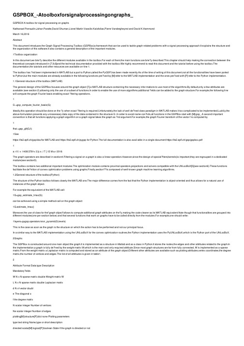
GSPBOX_-Atoolboxforsignalprocessingongraphs_GSPBOX:A toolbox for signal processing on graphsNathanael Perraudin,Johan Paratte,David Shuman,Lionel Martin Vassilis Kalofolias,Pierre Vandergheynst and David K.HammondMarch 16,2016AbstractThis document introduces the Graph Signal Processing Toolbox (GSPBox)a framework that can be used to tackle graph related problems with a signal processing approach.It explains the structure and the organization of this software.It also contains a general description of the important modules.1Toolbox organizationIn this document,we brie?y describe the different modules available in the toolbox.For each of them,the main functions are brie?y described.This chapter should help making the connection between the theoretical concepts introduced in [7,9,6]and the technical documentation provided with the toolbox.We highly recommend to read this document and the tutorial before using the toolbox.The documentation,the tutorials and other resources are available on-line 1.The toolbox has ?rst been implemented in MATLAB but a port to Python,called the PyGSP,has been made recently.As of the time of writing of this document,not all the functionalities have been ported to Python,but the main modules are already available.In the following,functions pre?xed by [M]:refer to the MATLAB implementation and the ones pre?xed with [P]:refer to the Python implementation. 1.1General structure of the toolbox (MATLAB)The general design of the GSPBox focuses around the graph object [7],a MATLAB structure containing the necessary infor-mations to use most of the algorithms.By default,only a few attributes are available (see section 2),allowing only the use of a subset of functions.In order to enable the use of more algorithms,additional ?elds can be added to the graph structure.For example,the following line will compute the graph Fourier basis enabling exact ?ltering operations.1G =gsp_compute_fourier_basis(G);Ideally,this operation should be done on the ?y when exact ?ltering is required.Unfortunately,the lack of well de?ned class paradigm in MATLAB makes it too complicated to be implemented.Luckily,the above formulation prevents any unnecessary data copy of the data contained in the structure G .In order to avoid name con?icts,all functions in the GSPBox start with [M]:gsp_.A second important convention is that all functions applying a graph algorithm on a graph signal takes the graph as ?rst argument.For example,the graph Fourier transform of the vector f is computed by1fhat =gsp_gft(G,f);1Seehttps://lts2.epfl.ch/gsp/doc/for MATLAB and https://lts2.epfl.ch/pygsp for Python.The full documentation is also avail-able in a single document:https://lts2.epfl.ch/gsp/gspbox.pdf1a r X i v :1408.5781v 2 [c s .I T ] 15 M a r 2016The graph operators are described in section4.Filtering a signal on a graph is also a linear operation.However,since the design of special?lters(kernels)is important,they are regrouped in a dedicated module(see section5).The toolbox contains two additional important modules.The optimization module contains proximal operators,projections and solvers compatible with the UNLocBoX[5](see section6).These functions facilitate the de?nition of convex optimization problems using graphs.Finally,section??is composed of well known graph machine learning algorithms.1.2General structure of the toolbox(Python)The structure of the Python toolbox follows closely the MATLAB one.The major difference comes from the fact that the Python implementation is object-oriented and thus allows for a natural use of instances of the graph object.For example the equivalent of the MATLAB call:1G=gsp_estimate_lmax(G);can be achieved using a simple method call on the graph object:1G.estimate_lmax()Moreover,the use of class for the"graph object"allows to compute additional graph attributes on the?y,making the code clearer as its MATLAB equivalent.Note though that functionalities are grouped into different modules(one per section below) and that several functions that work on graphs have to be called directly from the modules.For example,one should write:1layers=pygsp.operators.kron_pyramid(G,levels)This is the case as soon as the graph is the structure on which the action has to be performed and not our principal focus.In a similar way to the MATLAB implementation using the UNLocBoX for the convex optimization routines,the Python implementation uses the PyUNLocBoX,which is the Python port of the UNLocBoX. 2GraphsThe GSPBox is constructed around one main object:the graph.It is implemented as a structure in Matlab and as a class in Python.It stores the nodes,the edges and other attributes related to the graph.In the implementation,a graph is fully de?ned by the weight matrix W,which is the main and only required attribute.Since most graph structures are far from fully connected, W is implemented as a sparse matrix.From the weight matrix a Laplacian matrix is computed and stored as an attribute of the graph object.Different other attributes are available such as plotting attributes,vertex coordinates,the degree matrix,the number of vertices and edges.The list of all attributes is given in table1.2Attribute Format Data type DescriptionMandatory?eldsW N x N sparse matrix double Weight matrix WL N x N sparse matrix double Laplacian matrixd N x1vector double The diagonal of the degree matrixN scalar integer Number of verticesNe scalar integer Number of edgesplotting[M]:structure[P]:dict none Plotting parameterstype text string Name,type or short descriptiondirected scalar[M]:logical[P]:boolean State if the graph is directed or notlap_type text string Laplacian typeOptional?eldsA N x N sparse matrix[M]:logical[P]:boolean Adjacency matrixcoords N x2or N x3matrix double Vectors of coordinates in2D or3D.lmax scalar double Exact or estimated maximum eigenvalue U N x N matrix double Matrix of eigenvectorse N x1vector double Vector of eigenvaluesmu scalar double Graph coherenceTable1:Attributes of the graph objectThe easiest way to create a graph is the[M]:gsp_graph[P]:pygsp.graphs.Graph function which takes the weight matrix as input.This function initializes a graph structure by creating the graph Laplacian and other useful attributes.Note that by default the toolbox uses the combinatorial de?nition of the Laplacian operator.Other Laplacians can be computed using the[M]:gsp_create_laplacian[P]:pygsp.gutils.create_laplacian function.Please note that almost all functions are dependent of the Laplacian de?nition.As a result,it is important to select the correct de?nition at? rst.Many particular graphs are also available using helper functions such as:ring,path,comet,swiss roll,airfoil or two moons. In addition,functions are provided for usual non-deterministic graphs suchas:Erdos-Renyi,community,Stochastic Block Model or sensor networks graphs.Nearest Neighbors(NN)graphs form a class which is used in many applications and can be constructed from a set of points (or point cloud)using the[M]:gsp_nn_graph[P]:pygsp.graphs.NNGraph function.The function is highly tunable and can handle very large sets of points using FLANN[3].Two particular cases of NN graphs have their dedicated helper functions:3D point clouds and image patch-graphs.An example of the former can be seen in thefunction[M]:gsp_bunny[P]:pygsp.graphs.Bunny.As for the second,a graph can be created from an image by connecting similar patches of pixels together.The function[M]:gsp_patch_graph creates this graph.Parameters allow the resulting graph to vary between local and non-local and to use different distance functions [12,4].A few examples of the graphs are displayed in Figure1.3PlottingAs in many other domains,visualization is very important in graph signal processing.The most basic operation is to visualize graphs.This can be achieved using a call to thefunction[M]:gsp_plot_graph[P]:pygsp.plotting.plot_graph. In order to be displayable,a graph needs to have2D(or3D)coordinates(which is a?eld of the graph object).Some graphs do not possess default coordinates(e.g.Erdos-Renyi).The toolbox also contains routines to plot signals living on graphs.The function dedicated to this task is[M]:gsp_plot_ signal[P]:pygsp.plotting.plot_signal.For now,only1D signals are supported.By default,the value of the signal is displayed using a color coding,but bars can be displayed by passing parameters.3Figure 1:Examples of classical graphs :two moons (top left),community (top right),airfoil (bottom left)and sensor network (bottom right).The third visualization helper is a function to plot ?lters (in the spectral domain)which is called [M]:gsp_plot_filter [P]:pygsp.plotting.plot_filter .It also supports ?lter-banks and allows to automatically inspect the related frames.The results obtained using these three plotting functions are visible in Fig.2.4OperatorsThe module operators contains basics spectral graph functions such as Fourier transform,localization,gradient,divergence or pyramid decomposition.Since all operator are based on the Laplacian de? nition,the necessary underlying objects (attributes)are all stored into a single object:the graph.As a ?rst example,the graph Fourier transform [M]:gsp_gft [P]:pygsp.operators.gft requires the Fourier basis.This attribute can be computed with the function [M]:gsp_compute_fourier_basis[P]:/doc/c09ff3e90342a8956bec0975f46527d3240ca692.html pute_fourier_basis [9]that adds the ?elds U ,e and lmax to the graph structure.As a second example,since the gradient and divergence operate on the edges of the graph,a search on the edge matrix is needed to enable the use of these operators.It can be done with the routines [M]:gsp_adj2vec[P]:pygsp.operators.adj2vec .These operations take time and should4Figure 2:Visualization of graph and signals using plotting functions.NameEdge derivativefe (i,j )Laplacian matrix (operator)Available Undirected graph Combinatorial LaplacianW (i,j )(f (j )?f (i ))D ?WV Normalized Laplacian W (i,j ) f (j )√d (j )f (i )√d (i )D ?12(D ?W )D ?12V Directed graph Combinatorial LaplacianW (i,j )(f (j )?f (i ))12(D ++D ??W ?W ?)V Degree normalized Laplacian W (i,j ) f (j )√d ?(j )?f (i )√d +(i )I ?12D ?12+[W +W ?]D ?12V Distribution normalized Laplacianπ(i ) p (i,j )π(j )f (j )? p (i,j )π(i )f (i )12 Π12PΠ12+Π?12P ?Π12 VTable 2:Different de?nitions for graph Laplacian operator and their associated edge derivative.(For directed graph,d +,D +and d ?,D ?de?ne the out degree and in-degree of a node.π,Πis the stationary distribution of the graph and P is a normalized weight matrix W .For sake of clarity,exact de?nition of those quantities are not given here,but can be found in [14].)be performed only once.In MATLAB,these functions are called explicitly by the user beforehand.However,in Python they are automatically called when needed and the result stored as an attribute. The module operator also includes a Multi-scale Pyramid Transform for graph signals [6].Again,it works in two steps.Firstthe pyramid is precomputed with [M]:gsp_graph_multiresolution [P]:pygsp.operators.graph_multiresolution .Second the decomposition of a signal is performed with [M]:gsp_pyramid_analysis [P]:pygsp.operators.pyramid_analysis .The reconstruction uses [M]:gsp_pyramid_synthesis [P]:pygsp.operators.pyramid_synthesis .The Laplacian is a special operator stored as a sparse matrix in the ?eld L of the graph.Table 2summarizes the available de?nitions.We are planning to implement additional ones.5FiltersFilters are a special kind of linear operators that are so prominent in the toolbox that they deserve their own module [9,7,2,8,2].A ?lter is simply an anonymous function (in MATLAB)or a lambda function (in Python)acting element-by-element on the input.In MATLAB,a ?lter-bank is created simply by gathering these functions together into a cell array.For example,you would write:51%g(x)=x^2+sin(x)2g=@(x)x.^2+sin(x);3%h(x)=exp(-x)4h=@(x)exp(-x);5%Filterbank composed of g and h6fb={g,h};The toolbox contains many prede?ned design of?lter.They all start with[M]:gsp_design_in MATLAB and are in the module[P]:pygsp.filters in Python.Once a?lter(or a?lter-bank)is created,it can be applied to a signal with[M]: gsp_filter_analysis in MATLAB and a call to the method[P]:analysis of the?lter object in Python.Note that the toolbox uses accelerated algorithms to scale almost linearly with the number of sample[11].The available type of?lter design of the GSPBox can be classi?ed as:Wavelets(Filters are scaled version of a mother window)Gabor(Filters are shifted version of a mother window)Low passlter(Filters to de-noise a signal)High pass/Low pass separationlterbank(tight frame of2lters to separate the high frequencies from the low ones.No energy is lost in the process)Additionally,to adapt the?lter to the graph eigen-distribution,the warping function[M]:gsp_design_warped_translates [P]:pygsp.filters.WarpedTranslates can be used[10].6UNLocBoX BindingThis module contains special wrappers for the UNLocBoX[5].It allows to solve convex problems containing graph terms very easily[13,15,14,1].For example,the proximal operator of the graph TV norm is given by[M]:gsp_prox_tv.The optimization module contains also some prede?ned problems such as graph basis pursuit in[M]:gsp_solve_l1or wavelet de-noising in[M]:gsp_wavelet_dn.There is still active work on this module so it is expected to grow rapidly in the future releases of the toolbox.7Toolbox conventions7.1General conventionsAs much as possible,all small letters are used for vectors(or vector stacked into a matrix)and capital are reserved for matrices.A notable exception is the creation of nearest neighbors graphs.A variable should never have the same name as an already existing function in MATLAB or Python respectively.This makes the code easier to read and less prone to errors.This is a best coding practice in general,but since both languages allow the override of built-in functions,a special care is needed.All function names should be lowercase.This avoids a lot of confusion because some computer architectures respect upper/lower casing and others do not.As much as possible,functions are named after the action they perform,rather than the algorithm they use,or the person who invented it.No global variables.Global variables makes it harder to debug and the code is harder to parallelize.67.2MATLABAll function start by gsp_.The graph structure is always therst argument in the function call.Filters are always second.Finally,optional parameter are last.In the toolbox,we do use any argument helper functions.As a result,optional argument are generally stacked into a graph structure named param.If a transform works on a matrix,it will per default work along the columns.This is a standard in Matlab(fft does this, among many other functions).Function names are traditionally written in uppercase in MATLAB documentation.7.3PythonAll functions should be part of a module,there should be no call directly from pygsp([P]:pygsp.my_function).Inside a given module,functionalities can be further split in differentles regrouping those that are used in the same context.MATLAB’s matrix operations are sometimes ported in a different way that preserves the efciency of the code.When matrix operations are necessary,they are all performed through the numpy and scipy libraries.Since Python does not come with a plotting library,we support both matplotlib and pyqtgraph.One should install the required libraries on his own.If both are correctly installed,then pyqtgraph is favoured unless speci?cally speci?ed. AcknowledgementsWe would like to thanks all coding authors of the GSPBOX.The toolbox was ported in Python by Basile Chatillon,Alexandre Lafaye and Nicolas Rod.The toolbox was also improved by Nauman Shahid and Yann Sch?nenberger.References[1]M.Belkin,P.Niyogi,and V.Sindhwani.Manifold regularization:A geometric framework for learning from labeled and unlabeledexamples.The Journal of Machine Learning Research,7:2399–2434,2006.[2] D.K.Hammond,P.Vandergheynst,and R.Gribonval.Wavelets on graphs via spectral graph theory.Applied and ComputationalHarmonic Analysis,30(2):129–150,2011.[3]M.Muja and D.G.Lowe.Scalable nearest neighbor algorithms for high dimensional data.Pattern Analysis and Machine Intelligence,IEEE Transactions on,36,2014.[4]S.K.Narang,Y.H.Chao,and A.Ortega.Graph-wavelet?lterbanks for edge-aware image processing.In Statistical Signal ProcessingWorkshop(SSP),2012IEEE,pages141–144.IEEE,2012.[5]N.Perraudin,D.Shuman,G.Puy,and P.Vandergheynst.UNLocBoX A matlab convex optimization toolbox using proximal splittingmethods.ArXiv e-prints,Feb.2014.[6] D.I.Shuman,M.J.Faraji,and P.Vandergheynst.A multiscale pyramid transform for graph signals.arXiv preprint arXiv:1308.4942,2013.[7] D.I.Shuman,S.K.Narang,P.Frossard,A.Ortega,and P.Vandergheynst.The emerging?eld of signal processing on graphs:Extendinghigh-dimensional data analysis to networks and other irregular domains.Signal Processing Magazine,IEEE,30(3):83–98,2013.7[8] D.I.Shuman,B.Ricaud,and P.Vandergheynst.A windowed graph Fourier transform.Statistical Signal Processing Workshop(SSP),2012IEEE,pages133–136,2012.[9] D.I.Shuman,B.Ricaud,and P.Vandergheynst.Vertex-frequency analysis on graphs.arXiv preprint arXiv:1307.5708,2013.[10] D.I.Shuman,C.Wiesmeyr,N.Holighaus,and P.Vandergheynst.Spectrum-adapted tight graph wavelet and vertex-frequency frames.arXiv preprint arXiv:1311.0897,2013.[11] A.Susnjara,N.Perraudin,D.Kressner,and P.Vandergheynst.Accelerated?ltering on graphs using lanczos method.arXiv preprintarXiv:1509.04537,2015.[12] F.Zhang and E.R.Hancock.Graph spectral image smoothing using the heat kernel.Pattern Recognition,41(11):3328–3342,2008.[13] D.Zhou,O.Bousquet,/doc/c09ff3e90342a8956bec0975f46527d3240ca692.html l,J.Weston,and B.Sch?lkopf.Learning with local and global consistency.Advances in neural informationprocessing systems,16(16):321–328,2004.[14] D.Zhou,J.Huang,and B.Sch?lkopf.Learning from labeled and unlabeled data on a directed graph.In the22nd international conference,pages1036–1043,New York,New York,USA,2005.ACM Press.[15] D.Zhou and B.Sch?lkopf.A regularization framework for learning from graph data.2004.8。
convexhull函数

convexhull函数Convex Hull是计算凸包的一种常用算法,它是一个包围一组点的最小凸多边形。
凸包问题在计算机图形学、计算几何学和计算机视觉等领域中都有广泛的应用,用于解决诸如寻找最远点、点集包含关系判断等问题。
Convex Hull算法有多种实现方式,最常见的包括Graham Scan、Jarvis March以及Quick Hull。
下面将详细介绍Graham Scan算法。
1.算法思想:Graham Scan算法的基本思想是通过构建一个逆时针的类环排序,先找到最低的点(Y轴最小,如果有多个,则选择X轴最小的点),然后将其与其他所有点按照相对于最低点的极坐标进行排序。
排序后,按顺序将点加入凸包,同时保持凸包的有序性。
最后,返回生成的凸包。
2.算法步骤:a.找到最低点:遍历所有的点,找到Y轴最小值最小,并记录最低点的索引。
b.极坐标排序:除最低点外的其他点,根据其相对于最低点的极坐标进行排序。
c.构建凸包:依次将点加入凸包,同时根据凸包的有序性,维护凸包的结构。
d.返回凸包。
3.具体实现:下面是Graham Scan算法的伪代码实现:a.找到最低点:minPoint = points[0]for p in points:if p.y < minPoint.y or (p.y == minPoint.y and p.x < minPoint.x):minPoint = pb.极坐标排序:orientation = getOrientation(minPoint, point1, point2)if orientation == 0:return distSq(minPoint, point2) >= distSq(minPoint, point1) else:return orientation == 2c.构建凸包:hull = [minPoint]for i in range(1, len(sortedPoints)):while len(hull) > 1 and getOrientation(hull[-2], hull[-1], sortedPoints[i]) != 2:hull.pophull.append(sortedPoints[i])d.返回凸包:return hull4.时间复杂度:Graham Scan算法的时间复杂度为O(nlogn),其中n为点的数量。
convolutional layer的主要参数

convolutional layer的主要参数
主要参数如下:
1. Filters(滤波器):定义了每个卷积层使用的滤波器的数量。
每个滤波器都是一个小的矩阵,用于对输入数据进行局部特征提取。
2. Kernel Size(卷积核大小):指定了每个滤波器的大小。
常见的卷积核大小为3x3、5x5或7x7。
3. Stride(步幅):用于指定滤波器在输入数据上移动的步长。
较大的步长可以减小输出特征图的大小。
4. Padding(填充):在输入数据的边缘周围添加额外的像素,以便在卷积过程中保留输入特征图的尺寸。
常见的填充方式包括"valid"(无填充)和"same"(在边缘填充以保持输入和输出的尺寸相同)。
5. Activation Function(激活函数):用于引入非线性特征并增强卷积层的表达能力。
常见的激活函数包括ReLU、Sigmoid和Tanh 等。
6. Pooling(池化):用于减小特征图的尺寸,并减少后续层的计算量。
常见的池化方式包括最大池化(Max Pooling)和平均池化(Average Pooling)。
这些参数可以通过调整来优化模型的性能和效果。
惠普彩色激光打印机 Pro M454 和惠普彩色激光多功能一体机 Pro M479 维修手册说明书

Table -1 Revision history Revision number 1
Revision date 6/2019
Revision notes HP LaserJet Pro M454 HP LaserJet Pro MFP M479 Repair manual initial release
Additional service and support for HP internal personnel HP internal personnel, go to one of the following Web-based Interactive Search Engine (WISE) sites: Americas (AMS) – https:///wise/home/ams-enWISE - English – https:///wise/home/ams-esWISE - Spanish – https:///wise/home/ams-ptWISE - Portuguese – https:///wise/home/ams-frWISE - French Asia Pacific / Japan (APJ) ○ https:///wise/home/apj-enWISE - English ○ https:///wise/home/apj-jaWISE - Japanese ○ https:///wise/home/apj-koWISE - Korean ○ https:///wise/home/apj-zh-HansWISE - Chinese (simplified)
Find information about the following topics ● Service manuals ● Service advisories ● Up-to-date control panel message (CPMD) troubleshooting ● Install and configure ● Printer specifications ● Solutions for printer issues and emerging issues ● Remove and replace part instructions and videos ● Warranty and regulatory information
卷积层 全连接层 丢弃层 打平层 池化层 批量归一化层 模型参数

以下是您提到的各种层的解释和模型参数:
1. 卷积层(Convolutional Layer)
* 参数:卷积层的参数数量取决于其滤波器的数量和大小。
例如,如果一个卷积层有32个3x3的滤波器,那么该层的参数总数是\(32 \times 3 \times 3 = 288\)(不包括偏置项)。
2. 全连接层(Fully Connected Layer)
* 参数:全连接层的参数数量是节点数和输入特征数量的乘积。
例如,如果全连接层有100个节点,并且输入特征的数量是784(例如,MNIST数据集),那么该层的参数总数是\(100 \times 784 = 78400\)。
3. 丢弃层(Dropout Layer)
* 参数:丢弃层本身没有参数。
它通过随机关闭网络中的某些节点来防止过拟合,并提高模型的泛化能力。
4. 打平层(Flatten Layer)
* 参数:打平层也没有参数。
它的主要目的是将多维的输入一维化,以便可以将其传递给全连接层。
5. 池化层(Pooling Layer)
* 参数:池化层也没有参数。
池化层的目的是减少数据的维度,通常在卷积层之后使用,以减少计算量并提高模型的泛化能力。
6. 批量归一化层(Batch Normalization Layer)
* 参数:批量归一化层有少量的参数用于计算均值和方差,但这些参数在训练过程中会被学习到。
此外,它还有可学习的线性变换的权重和偏置项。
这些层在神经网络中起到了不同的作用,并且各有其特殊的参数。
在实际应用中,需要根据任务和数据集的特性来选择和设计合适的网络结构。
- 1、下载文档前请自行甄别文档内容的完整性,平台不提供额外的编辑、内容补充、找答案等附加服务。
- 2、"仅部分预览"的文档,不可在线预览部分如存在完整性等问题,可反馈申请退款(可完整预览的文档不适用该条件!)。
- 3、如文档侵犯您的权益,请联系客服反馈,我们会尽快为您处理(人工客服工作时间:9:00-18:30)。
Convex Upper and Lower Bounds forPresent Value FunctionsD.Vyncke∗M.Goovaerts†J.Dhaene‡AbstractIn this paper we present an efficient methodology for approximating thedistribution function of the net present value of a series of cash-flows,whenthe discounting is presented by a stochastic differential equation as in theVasicek model and in the Ho-Lee model.Upper and lower bounds in con-vexity order are obtained.The high accuracy of the method is illustratedfor cash-flows for which no analytical results are available.1IntroductionWhen determining the present value of a series of n payments c i at timesτi (i=1,...,n),one has to define a discount process X(τ).The present value ofthis series is then given byV0=ni=1c i e−X(τi).(1)To determine the cumulative distribution function(cdf)of this random vari-able(rv),one has to cope with a standard problem:the summation of rvs with marginal cdfs of the same type need not(and often will not)produce a cdf of that type.Secondly,the dependence structure of the rvs X(τi)is not known or hard to obtain in general.Although we could approximate the cdf via Monte Carlo simulation when the dependence structure of the X(τi)is given,this would be very time-consuming.Moreover,if we want to estimate a high quantile(e.g. Value-at-Risk)accurately,we should increase the sample size–and consequently the computation time–ing results from actuarial risk theory on comonotonic risks,we can however obtain an easily computable upper bound for V0.In addition,Jensen’s inequality combined with the theory on comonotonic risks provides a tool for obtaining a lower bound.∗K.U.Leuven†K.U.Leuven,U.v.Amsterdam‡K.U.Leuven,U.v.Amsterdam,Universiteit Antwerpen1In this paper we will define the discount factors as follows.We write X(τ)asX(τ)=τr(s)ds,(2)henceV0=ni=1c i exp−τir(s)ds,(3)and consider two types of models for r(s).In thefirst model,the stochastic differential equation for describing the behaviour of r(s)is the same as the one for the instantaneous interest rate in the Vasicek(1977)model:dr=(α−βr)dt+γdW,(4)whereα,βandγare non-negative constants and W represents a standard Wiener process.Replacingαby a non-negative functionα(t)of time,as in the Ho-Lee (1986)model yields a second model:dr=α(t)dt+γdW.(5)In the present paper analytical upper and lower bounds for the distribution func-tion of V0are obtained.They are shown to be practically applicable due to the very small relative error bounds.Random variables of this type arise in modern actuarial situations where e.g.discounting is taken into account in the evaluation of the distribution of IBNR provisions.In the case offinancial reinsurance it provides the distribution of the experience account and as such it enables the determination of thefinal premium of this type of reinsurance.Knowing the dis-tribution of V0,provides a tool for the determination of the”fair value”as well as the”supervisory value”of a portfolio of risks.Moreover it avoids simulations in solvency calculations and it helps for the determination of embedded value and appraisal value.Our methodology only requires the knowledge of the distribution functions of the X(τi)and does not take into account the dependence structure between these random variables.Allowing for all kinds of dependence structures,which often cannot be measured because of the incomplete statistical basis,of course has an influence on the distribution function of V0.Replacing the unknown cdf of V0by the upper bound(in convex order sense)is a safe strategy in the sense that all risk averse decision makers would prefer the original(unknown)cdf.On the other hand,the lower bound gives us an idea of the high accuracy of the approximation.22Convex Upper BoundIn the actuarialfield it is common practice to replace the cdf of V0by a”less favourable”one.Of course the new cdf should be easier to determine,see e.g. Goovaerts e.a.(1986).To formalise the concept”less favourable”,we make use of the convex order.Definition1A rv V is smaller than a rv W in the convex order ifE[φ(V)]≤E[φ(W)]for all convex functionsφ:R→R.This is denoted as V≤cx W.In terms of utility theory,V≤cx W means that the rv V is preferred to the rv W by all risk averse decision makers,i.e.E[u(−V)]≥E[u(−W)]for all concave utility functions u.Replacing the cdf of V by the cdf of W can therefore be considered as a prudent strategy.A closely related order is the stop-loss order.Definition2A rv V is smaller than a rv W in the stop-loss order ifE[V−d]+≤E[W−d]+for all d.This is denoted as V≤s W.In Shaked&Shanthikumar(1994)it is proven that the convex order incorporates the stop-loss order:V≤cx W⇐⇒V≤s WEV=EW(6)We will now introduce the concepts of a Fr´e chet space and comonotonic risks, which will enable us to construct an upper bound for V0.Definition3The Fr´e chet space R n(F1,...,F n)determined by the(univariate) distribution functions F1,...,F n is the class of all n-variate distribution functions F(or the corresponding rvs)with marginals F1,...,F n.In the Fr´e chet space R n(F1,...,F n)any rv X is constrained from above byF X(x)≤min{F1(x1),F2(x2),...,F n(x n)}=:W n(x),∀x∈R nA comonotone risk is a rv with cdf W n,see e.g.D haene et al(1997):Definition4A random vector(X1,...,X n)is said to be comonotone(the rvs X1,...,X n are said to be mutually comonotone)if any of the following equivalent conditions hold:31.For the n-variate cdf we haveF X(x)=min{F1(x1),F2(x2),...,F n(x n)},∀x∈R n;2.There exist a rv Z and non-decreasing functions g1,...,g n:R→R suchthat(X1,...,X n)d=(g1(Z),...,g n(Z));3.For any rv U uniformily distributed on[0,1],we have(X1,...,X n)d=(F−11(U),...,F−1n(U)).As usual,”d=”denotes equality in distribution and F−1represents the inverse of the cdf F defined asF−1X(p)=inf{x∈R|F X(x)≥p},p∈[0,1].It can be seen from condition2that comonotonic rvs possess a very strong positive dependence:increasing one of the X i will lead to an increase of all other rvs X j involved.These special rvs will provide us with a tool to construct a close upper bound for V0,see Goovaerts et al(2000).Theorem1Let X=(X1,...,X n)be a n-dimensional rv with marginals F1,...,F n. Further,let U be a rv,uniformly distributed on[0,1].Finally,letφ1,...,φn be non-negative and non-increasing functions.Thenφ1(X1)+···+φn(X n)≤cxφ1(F−11(U))+···+φn(F−1n(U)).(7) Proof.In Goovaerts&D haene(1999),it is shown thatni=1φi(X i)≤sni=1φi(F−1i(U)).Because(X1,...,X n)and(F−11(U),...,F−1n(U))have the same marginals, ni=1φi(X i)and ni=1φi(F−1i(U))have the same mean.Equation(6)then completes theproof.Settingφi(X):=c i exp(−X(τi)),we obtain the convex upper boundW=ni=1φi(F−1X(τi)(U))=ni=1c i exp(−F−1X(τi)(U)).(8)To compute the cdf of W,we can use the additivity of the inverse cdfs of comono-tonic risks.4Proposition1Let Y1,...,Y n be n comonotonic risks with marginals F1,...,F n. ThenF−1 S (p)=ni=1F−1i(p),p∈[0,1],with S=Y1+...+Y n.For a proof of this result,we refer the interested reader to D ennenberg(1994). Remark that,for any strictly decreasing functionφand any cdf F X,φ(F−1X (p))=F−1φ(X)(1−p),p∈[0,1].So,for strictly positive cash-flows c i and strictly increasing F X(τi),the tail functionF W:=1−F W is implicitely given byni=1φi(F−1X(τi)(F W(x)))=x.(9)Notice that we only need to know the inverse marginal cdfs F−1X(τi)to computethe upper bound.If all c i<0,then F W is implicitely given byni=1φi(F−1X(τi)(F W(x)))=x.(10)The case when certain c i are negative and other are positive is considered in Goovaerts et al(2000).Theorem1can also be used to determine an upper bound for the price of an arithmetic Asian option,see Simon et al(2000).3Convex Lower BoundStarting from Jensen’s inequality for conditional expectations,E[f(V)|Z]≥f(E[V|Z]),(11) where f:R→R is a convex function,we can derive a convex lower bound for V0.This inequality has also been used by Rogers&Shi(1995)to obtain a lower bound for the price of an Asian option,while Feynman&Hibbs(1965) applied it to introduce a variational result for essentially the same quantity,c.q. the partition matrix,an important quantity in mathematical physics.Proposition2For any two rvs Y and Z,let L:=E(Y|Z).ThenL≤cx Y(12)5Proof.As (·)+=max(·,0)is a convex function,we find for all kE [Y −k ]+=E [E ((Y −k )+|Z )]≥E [E (Y −k |Z )]+=E [L −k ]+Furthermore,L and Y have the same mean,so again equation (6)completes the proof.Replacing Y by V 0and choosing an appropriate conditioning variable Z ,we get an expression for the stop-loss transform E (L −k )+of the convex lower bound L .To compute the cdf F L out of E (L −k )+,remark that E (X −k )+= +∞k(x −k )dF X (x ),hence d dk E (X −k )+=− +∞k dF X (x )=F X (k )−1.(13)4Application:Vasicek &Ho-Lee ModelSolving the stochastic differential equation for the Vasicek model results in r (s )=e −βs r (0)+αβ(1−e −βs )+γe −βss 0e βu dW (u ),(14)∼N e −βs r (0)+αβ(1−e −βs ),γ22β(1−e −2βs ). (15)Straightforward calculus then yields,for X (τ):= τ0r (s )ds ,X (τ)=αβτ+1β(r (0)−αβ)(1−e −βτ)+γβ τ0(1−e β(u −τ))dW (u ),which in turn has a normal distribution with meanµ(τ)=αβτ+1β(r (0)−αβ)(1−e −βτ)and varianceσ2(τ)=γ2β τ−2β(1−e −βτ)+12β(1−e −2βτ) .For the Ho-Lee model we getr (s )=r (0)+ s 0α(u )du +γW (s ),(16)∼N r (0)+ s0α(u )du,γ2s .(17)6Consequently,X(τ)is normally distributed with meanµ(τ)=r(0)τ+ϕα(τ)and varianceσ2(τ)=γ2τ3 3,where we used the abbreviationϕα(τ):= τα(u)(τ−u)du.The convex upper bound for V0for both models follows fromni=0c i exp−µ(τi)−σ(τi)Φ−1(F W(k))=k(18)whereΦdenotes the standard normal cdf.Equivalently,F W(k)=1−Φ(u k)(19) with u k determined byni=0c i exp{−µ(τi)−σ(τi)u k}=k.(20)To compute the convex lower bound,wefirst have to choose a conditioning vari-able Z.Therefore,defineIδ:=−δX(τ)dτ,which is clearly again normally distributed,say,with meanµδand varianceσ2δ.Now we chooseZδ:=Iδ−µδσδ∼N(0,1),(21)as conditioning variable.Recall that when a normal rv−X(τ)is conditioned on a standard normal rv Zδ,it remains normal with meanE(−X(τ)|Zδ)=−E(X(τ))+kτ,δZδand varianceV ar(−X(τ)|Zδ)=V ar(X(τ))−k2τ,δ,wherekτ,δ=Cov(−X(τ),Zδ)=1σδδCov(X(τ),X(ν))dν. 7The stop-loss transform of the lower bound L is given by E (L −k )+=E En i =1c i e −X (τi )|Z δ −k +=En i =1c i E e −X (τi )|Z δ −k +=E n i =1c i exp −µ(τi )+k τi ,δZ δ+12(σ2(τi )−k 2τi ,δ) −k += 10 n i =1c i exp −µ(τi )+k τi ,δΦ−1(u )+12(σ2(τi )−k 2τi ,δ) −k +du Notice that the integrand is a non-decreasing function of u ,at least if c i ≥0and k τi ,δ≥0(i =1,...,n ).This means that the integrand equals zero for all u ≤u k ,with u k determined byn i =1c i exp −µ(τi )+k τi ,δΦ−1(u k )+12(σ2(τi )−k 2τi ,δ) =k.(22)ConsequentlyE (L −k )+=1u k n i =1c i exp −µ(τi )+k τi ,δΦ−1(u )+12(σ2(τi )−k 2τi ,δ) −k du and d dk E (L −k )+= 1u k (−1)du =u k −1.Finally,using equation (13),we findF L (k )=u k .(23)If however c i <0,∀i ,then d dkE (L −k )+= u k 0(−1)du =−u k ,and F L (k )=1−u k .For the Vasicek model,some lengthy yet simple calculations yield k τ,δ=1σδ δ0γ2β2 (τ∧ν)−1β(e β(τ∧ν)−1)(e −βτ+e −βν)+12β(e β(τ∧ν)−e −β(τ∧ν)) dν=1σδγ2β2 τδ−τ22+1β(δ+e −βδβ)(e −βτ−1)−12β2(e −2βτ+1) 8whereτ≤δandσδ=γββδ2βδ3−1−δ2e−βδ−1−12βe−2βδ−112.Remark thatCov(r(u),r(s))=e−β(u+s)γ22βe2β(u∧s)−1≥0which implies the positivity of kτ,δ.Analogous,for the Ho-Lee model we getkτ,δ=1σδδγ22(τ∧ν)2(τ+ν)−23γ2(τ∧ν)3dν=γ2τ22σδτ212−τδ3+δ22whereτ≤δandσδ=γδ22δ/5.The kτi,δare here also positive,becauseCov(r(u),r(s))=γ2(u∧s)≥0.5Accuracy of the boundsIn this section we investigate the accuracy of the proposed bounds for the present value function V0,by comparing their cdf to the empirical cdf obtained with Monte Carlo simulation.We also construct a QQ-plot to visualise the goodness-of-fit.Finally,we determine the maximum stop-loss error,relatively to the ex-pected value of V0,by calculating the stop-loss premiums of the upper and lower bound respectively:E(W−k)+−E(L−k)+E(V0)Thefirst case considered is the Vasicek model with parametersα=0.0038438,β=0.044688andγ=0.0015313,see D e Winne(1995).We set c i=100,τi=i (i=1,...,30)and choose r(0)=0.08,δ=30.Figure1shows the distribution functions and the corresponding QQ-plots of the upper and lower bounds,compared to the empirical distribution based on 10000randomly generated,normally distributed vectors.The distribution func-tions are remarkably close to each other and enclose the simulated cdf nicely. This is confirmed by the QQ-plot where we also see that the comonotonic upper9bound has somewhat heavier tails.In figure 2we plot the upper and lower stop-loss premiums,E (W −k )+and E (L −k )+respectively,for several retentions k .The vertical line indicates the mean present value E (V 0)=1074.987.For the maximal value of the maximum relative stop-loss error,we find max k E (W −k )+−E (L −k )+E (V 0)≈0.08%.We now construct a Ho-Lee model where,besides a lineair part,r (·)consists of a harmonically damped oscillation and some normally distributed error.Therefore,we defineα(τ):=B +Ae −gτ[ωcos(ωτ)−g sin(ωτ)]with γ=0.01,A =0.003,B =0.01,g =0.01and w =3.Hence,ϕα(τ)=Bτ22+Aωg +ω−Ae −gτ[ωcos(ωτ)+g sin(ωτ)]g +ωAgain,we assume equal payments c i =100at times τi =i (i =1,...,30)and choose δ=30.The initial interest rate r (0)is set to 0.5,so E (V 0)=839.4933.Figures 3and 4again indicate the high accuracy of the bounds:e.g.the maxi-mum relative stop-loss error stays below 0.6%.Intuitively,we expect the bounds to perform worse when the payments c i are no longer constant or when γincreases.We therefore revisit the Vasicek model and set c i =i .Moreover,we increase γby a factor 10,so E (V 0)=121.4577.Despite the absence of the c i in the conditioning variable Z δ,both upper and lower bounds remain excellent approximations (see figures 5en 6).References[1]Bingham N.H.&Kiesel R.,1998,Risk-Neutral Valuation,Pricing and Hedg-ing of Financial Derivatives ,Springer-Verlag London.[2]D e Winne R.,1995,The Discretization Bias for Processes of the Short-TermInterest Rate:An Empirical Analysis ,D iscussion Paper CORE 9564.[3]D ennenberg D .,1994,Non-Additive Measure and Integral ,Kluwer AcademicPublishers,Boston.[4]D haene J.,Wang S.,Young V.&Goovaerts M.J.,1997,Comonotonicityand Maximal Stop-Loss Premiums ,Research Report 9730,D epartment of Applied Economics K.U.Leuven.[5]Feynman R.P.&Hibbs A.R.,1965,Quantum Mechanics and Path-Integrals ,Mc.Graw Hill Book Company,New York.10[6]Goovaerts M.J.&D haene J.,1999,Supermodular ordering and stochasticannuities,Insurance:Mathematics and Economics,24,p.281-290.[7]Goovaerts M.J.,D haene J.&D e Schepper A.,2000,Stochastic upper boundsfor present value functions,Journal of Risk and Insurance,forthcoming. [8]Ho T.&Lee S.,1986,Term Structure Movements and Pricing Interest RateContingent Claims,Journal of Finance,41.[9]Rogers L.&Shi Z.,1995,The Value of an Asian Option,Journal of AppliedProbability,32,p.1077-1088.[10]Shaked M.&Shanthikumar J.G.,1994,Stochastic orders and their applica-tions,Academic press,p.545.[11]Simon S.,Goovaerts M.J.&D haene J.,2000,An easy computable upperbound for the price of an arithmetic Asian option,Insurance:Mathematics &Economics,forthcoming.[12]Vasicek O.,1977,An Equilibrium Characterization of the Term Structure,Journal of Financial Economics,5,p.177-188.11present valuec u m .d i s t r .1000105011001150Upper Bound, Lower Bound & Empirical Distribution (Vasicek model)(a)Upper (—)&lower (--)bound vs.Monte Carlo simulation (···)10201040106010801100112011401020104010601080110011201140QQ-plot (Vasicek model)(b)Upper ( )&lower (◦)quantiles vs.Monte Carlo quantilesFigure 1:Distribution function and QQ-plot of the upper &lower bounds (Va-sicek model),compared to Monte Carlo simulation.12retentions t o p -l o s s p r e m i u m1050110011501200Upper & lower stop-loss premium (Vasicek model)(a)Stop-loss premiumsretentionm a x . r e l a t i v e s t o p -l o s s e r r o r10501100115012000.00.00020.00040.00060.0008Max. relative stop-loss error (Vasicek model)(b)Maximum relative stop-loss errorFigure 2:Stop-loss premiums for the upper &lower bounds and the corresponding maximum relative stop-loss error (Vasicek model)13pricec u m .d i s t r .600800100012001400Upper Bound, Lower Bound & Empirical Distribution (Ho-Lee model)(a)Upper (—)&lower (--)bound vs.Monte Carlo simulation (···)70080090010001100700800900100011001200QQ-plot (Ho-Lee model)(b)Upper ( )&lower (◦)quantiles vs.Monte Carlo quantilesFigure 3:Distribution function and QQ-plot of the upper &lower bounds (Ho-Lee model),compared to Monte Carlo simulation14retentions t o p -l o s s p r e m i u m800100012001400Upper & lower stop-loss premium (Ho-Lee model)(a)Stop-loss premiumsretentionm a x . r e l a t i v e s t o p -l o s s e r r o r8001000120014000.00.0010.0020.0030.0040.005Max. relative stop-loss error (Ho-Lee model)(b)Maximum relative stop-loss errorFigure 4:Stop-loss premiums for the upper &lower bounds and the corresponding maximum relative stop-loss error (Ho-Lee model)15present valuec u m .d i s t r .100200300400Upper Bound, Lower Bound & Empirical Distribution (Vasicek model)(a)Upper (—)&lower (--)bound vs.Monte Carlo simulation (···)50100150200250300350100200300QQ-plot (Vasicek model)(b)Upper ( )&lower (◦)quantiles vs.Monte Carlo quantilesFigure 5:Distribution function and QQ-plot of the upper &lower bounds (Va-sicek model),compared to Monte Carlo simulation16retentions t o p -l o s s p r e m i u m100200300400500600700Upper & lower stop-loss premium (Vasicek model)(a)Stop-loss premiumsretentionm a x . r e l a t i v e s t o p -l o s s e r r o r1002003004005006007000.00.0020.0040.006Max. relative stop-loss error (Vasicek model)(b)Maximum relative stop-loss errorFigure 6:Stop-loss premiums for the upper &lower bounds and the corresponding maximum relative stop-loss error (Vasicek model)17。