Mixing of Primordial Gas in Lyman Break Galaxies

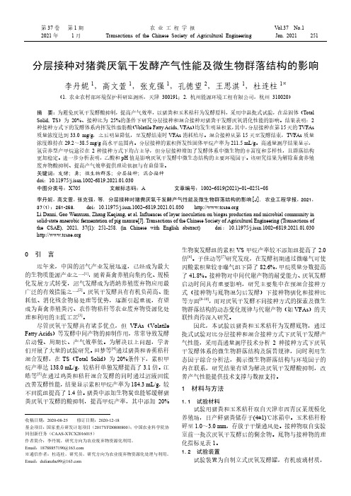
a r X i v :a s t r o -p h /0611376v 1 13 N o v 2006ApJ Letters,in pressPreprint typeset using L A T E X style emulateapj v.10/09/06MIXING OF PRIMORDIAL GAS IN LYMAN BREAK GALAXIESLiubin Pan and John ScaloAstronomy Department,University of Texas at Austin,Austin,TXpanlb@;scalo@ApJ Letters,in pressABSTRACTMotivated by an interpretation of z ∼3objects by Jimenez and Haiman (2006),we examine processes that control the fraction of primordial (Z =0)gas,and so primordial stars,in high-SFR Lyman break galaxies.A primordial fraction different from 1or 0requires microscopic diffusion catalyzed by a velocity field with timescale comparable to the duration of star formation.The only process we found that satisfies this requirement for LBGs without fine-tuning is turbulence-enhanced mixing induced by exponential stretching and compressing of metal-rich ejecta.The time-dependence of the primordial fraction for this model is calculated.We show that conclusions for all the models discussed here are virtually independent of the IMF,including extremely top-heavy IMFs.Subject headings:ISM:evolution–galaxies:abundances–galaxies:evolution–galaxies:ISM–turbulence1.INTRODUCTIONGalaxies begin their lives with entirely primordial (Z =0)gas.As they age,metal production and mixing can only reduce the primordial gas fraction.We have ex-plored the expected time dependence of the primordial fraction for various types of mixing and chemical evolu-tion processes using a kinetic equation for the evolution of the abundance distribution.The present Letter ad-dresses the narrower question of whether any models for mixing and chemical evolution predict this transforma-tion occurs at an accessible redshift.Jimenez and Haiman (2006)(hereafter JH)showed that several UV properties of a variety of objects,mostly Lyman break galaxies (LBGs),at redshift z ∼3,can all be understood if these objects contain a substantial fraction,about 10to 50percent,of massive stars withessentially zero metallicity (Z ∼<10−5Z ⊙;we use Z and metallicity indiscriminantly here).These UV prop-erties cannot together be explained by a top-heavy IMF,and require Z =0stars;a top-heavy IMF is not re-quired.Massive stars have short lifetimes,so their metal abundances reflect that of the concomitant gas.Thus,if JH are correct,a substantial fraction of the interstel-lar medium of these galaxies,with star formation ages a few hundred million years,has not been polluted by any products of nucleosynthesis.1Motivated by JH and other suggestions for Z =0stars (Malhotra &Rhoads 2002;Shimasaku et al.2006),and the fact that during some early period in the lives of all galaxies a transformation from primordial to non-primordial must occur,leaving spectrophotometric sig-natures (JH;see Schaerer 2003),we examined the viabil-ity of a number of models for this transformation.A change in the primordial fraction requires micro-scopic diffusion enhanced by a complex velocity field,1The existence of Z =0gas requires an IMF deficient in stars with M ∼<1M ⊙.Otherwise the number of low-mass stars observable today would be large,contradicting observational limits on the star fraction with very small Z (see Oey 2003)by several orders of magnitude.We discuss the effects of different IMFs below,where we show that all our conclusions are independent of the IMF as long as it satisfies the requirement M ∼>1M ⊙.such as instabilities in swept-up supernova shells or aturbulent interstellar medium (ISM),along with disper-sal of nucleosythesis products over many kpc,involving a scale range of ∼105.Existing hydrodynamic simulations in a cosmological context (e.g.,Governato et al.2004;Scannapieco et al.2005)therefore cannot represent the transition of the primordial gas or mixing in general,since they adopt mixing rules that arbitrarily spread met-als among nearest neighbor cells or SPH particles.The only hydrodynamic simulations of true mixing of tracers in galaxies were concerned either with turbulent disper-sal of mean metallicity,not mixing (Klessen &Lin 2003),or mixing of initial spatially periodic inhomogeneities by numerical diffusivity in a turbulent galaxy with no con-tinuing source of metals (de Avillez &Mac Low 2002).Instead of simulations,the arguments given here are phenomenological,in order to clarify the essentials for each physical process.A detailed discussion is given elsewhere (Pan and Scalo 2006,hereafter PS)using a formal probability distribution evolution equation.Here we report that most processes we examined are either far too fast or slow to partially erase the primordial frac-tion (Sec.2),except for mixing by turbulence-enhanced diffusivity based on exponential stretching of blobs of nucleosynthesis products,discussed in Sec.3.22.ESTIMATES OF TIMESCALES FOR MIXINGPROCESSES2.1.Star Formation AgeThe existence of a primordial gas fraction P (t )that is not nearly unity or zero,i.e.,both P (t )and 1−P (t )are significantly larger than zero,a condition we refer to as a “significant”or “intermediate”primordial fraction,requires a mixing or depletion process whose character-istic timescale is comparable to the star formation (SF)age,the time since SF began.If the mixing timescale is much smaller,P (t )will be nearly zero;if it is much2A recent estimate of the effect of SN mixing (sec. 2.4below)on the primordial fraction at high redshift (Tumlinson 2006)ap-parently used a shell mass much larger than found in analytical and numerical calculations of supernova remnant evolution (see Thornton et al.1998;Hanayama &Tomisaka 2006).2Pan&Scalolarger,P(t)will remain near unity.SF ages for LBGs and likely-related objects at somewhat different redshifts have been estimated by Papovich et al.(2001),Shapley et al.(2001),Erb et al.(2006)and others,using galaxy evolution models that assume an exponentially decreas-ing SFR that began at some time in the past.Although there is much variation,median SF ages are3×108yr. These SF ages cannot be significantly different for a number of reasons.The lookback times of about11.5 Gyr for z=3imply a strict upper limit to the SF age of 2Gyr,and a more likely upper limit of1.5Gyr(corre-sponding to z∼8).The irregular morphologies of the LBGs(Giavalisco2002)suggest that LBGs are in the process of formation,accumulating large fragments of gas and stars through mergers(Conselice2006),and proba-bly undergoing one of theirfirst major bursts of SF;star-burst populations have durations,estimated from statis-tics(Kennicutt et al.1987;Nikolic et al.2004),model-ing of integrated light features(Marcillac et al.2006), and theoretical arguments(see Leitherer2001),that are similar to the estimates in LBGs.Finally,ages much greater than3×108yr would produce greater metallic-ity than observed(see Giavalisco2002).We assume star formation has been a continuous func-tion of time.If instead the SFR preceding or during the present episode consists of bursts of shorter duration, most of our arguments remain unchanged if the SF age is replaced by the accumulated duration of SF.2.2.Depletion of the Primordial Fraction by Sources The JH result of10-50%primordial at z∼3seems surprising,but actually galaxies should remain almost completely primordial for billions of years in the absence of microscopic diffusivity.SN metal production slowly depletes primordial gas by transferring it from a Z=0 delta function in the Z probability distribution(pdf)to another delta function at a much larger Z,the source metallicity Z s averaged over the IMF(∼0.1assuming the hot ejecta are well mixed).Intermediate values of Z cannot be reached without diffusivity.This suggests the simplest explanation for an inter-mediate primordial fraction in LBGs:50to90%of the primordial gas passed through stars that became SNe. The timescale for this process is the source timescale,τsrc=M gas/BR SN,where B is the star formation rate and R SN is the returned fraction from SNe aver-aged over the IMF.We take the total gas mass M gas as 5×1010M⊙,extrapolated from gas masses estimated in the z∼2UV-selected sample of Erb et al.(2006). From a number of studies,we adopt a median SFR of100 M⊙/yr for LBGs at z∼3assuming the IMF lower limit M l=0.1(Papovich et al.2001;Shapley et al.2001; Giavalisco2002;Erb et al.2006;Yan et al.2006).For this M l,we calculate R SN≈0.1for various IMFs using the ejected masses given in Woosley&Weaver(1995), Meynet&Maeder(2002)and Nomoto et al.(2006),find-ing little dependence on metallicity,including Z=0,and 20-30%variation between studies.Variations in the form of the IMF change the SFR by∼50%,with only a slight effect on R SN.The source timescale is thenτsrc=5 Gyr,within a factor of a few considering the uncertainty in the SFR and M gas,too large to affect the primordial fraction.We examined the IMF-dependence ofτsrc.There are two nonstandard IMFs that are especially relevant. 1. Intermediate primordial fractions require that the IMF lower limit M l∼>1M⊙to avoid too many Z=0stars observable today.Such a cutoffdoes not affect the source timescale:The empirical SFRs are based on integrated light from massive stars corrected for the rest of the IMF, and the resulting decrease of the SFR due to the cutoffis exactly compensated by the increase of the mass ejected by supernovae per unit mass of stars formed R SN.This IMF-independence ofτsrc holds for any cutoffsmaller than the lower mass limit for SNe,∼8M⊙.By the same argument,such a cutoffdoes not overproduce metallicity.2.A perennially popular IMF for Z=0star formation consists of only very massive stars(VMS)due to the Jeans mass resulting from H2cooling(Hutchins1976; see Bromm and Larson2004)although it has been ques-tioned on a number of grounds(Silk&Langer2006). Comparing Hαemission per unit SFR for a VMS IMF (50-500)M⊙of Z=0stars in Schaerer(2003)with the same quantity for a(0.1-100)M⊙IMF in Kennicutt (1998),both for a Salpeter IMF(for illustration only), the SFR for a VMS IMF is26times smaller.Assuming only stars in the range130-260M⊙explode as pair in-stability SNe(Woosley et al.2002),wefind R SN=0.27, soτsrc=50Gyr,an order of magnitude larger than the normal IMF case.These results strengthen our conclusion that the forma-tion of massive stars is far too slow to deplete primordial gas significantly in the available time.2.3.Filling the Gap by DiffusionWithout a process to spread metals into the“gap”be-tween the Z s peak and the primordial Z=0peak,P(t) would remain near unity for billions of years.The only physical process that canfill this gap is microscopic diffu-sivity.However an estimate of the rate at which diffusiv-ity from random sources could pollute primordial gas in LBGs,using diffusion lengths for the cold neutral,warm neutral,and warm ionized ISM similar to those in Oey (2003),shows that the fraction of the mass of a galaxy mixed in time t is only∼10−5(t/0.5Gyr)5/2,so diffu-sivity by itself cannot pollute more than a tiny fraction of the primordial gas over the estimated SF ages.To reduce the primordial fraction,a velocityfield is required to catalyze diffusivity.However a velocityfield cannot by itself affect the global metallicity distribution or primordial fraction,or mix at all:Displacement of fluid parcels of different Z by the velocityfield conserves their volumes and thus volume fractions(or mass frac-tions for compressibleflows),replacing one by another in space,having no effect on the Z distribution.This can be shown rigorously using a metallicity pdf equation (PS).A velocityfield can only enhance mixing by spa-tially ramifying the Zfield for diffusion to operate on small scales.Models that mix by sweeping of gas by SN or SB shells,cloud motions,differential rotation,or“tur-bulent diffusion”are unphysical without recognition that they are implicit models for microscopic diffusion.2.4.Several Catalyzing Velocity Fields Expanding SNRs and superbubbles(SBs)are the main agents of mixing in many sequential enrichment inho-mogeneous chemical evolution models(Reeves1972;seePrimordial Gas in LBGs3Tsujimoto et al.1999;Oey2000;Argast et al.2000; Saleh et al.2006).Shells can mix,but only if instabilities allow diffusion to mix swept-up gas with new products of nucleosynthesis.Assuming this oc-curs,each SNR sweeps up and mixes a mass M sw∼2×104M⊙for Z=0gas(Thornton et al.1998; Hanayama&Tomisaka2006).The time to sweep up primordial ISM isτsw=M gas/(νSN M sw),where the SN rateνSN=ǫB/ M∗ .For an IMF with mass range (0.1,100)M⊙and indices(-0.4,-1.7)below and above 1M⊙the number fractionǫof stars that become SNe is0.004and the average stellar mass M∗ =0.6,so νSN=0.7/yr andτsw=3×106yr.Equivalently,the ac-cumulated volumefilling factor NQ=t/τsw(Oey2000), so P=exp(−t/τsw)=exp(−NQ)and it is impossible to preserve primordial gas in LBGs for longer than∼1% of the observed SF ages∼3×108yr,unless the mixing efficiency is artificially tuned to1%,in which case the model predicts too large a present-day scatter in metal-licity compared to observations.Superbubbles have a smaller frequency,but sweep up more gas,producing an almost identical result.Spatial clustering and infalling Z=0gas also do not affect the conclusion.These points are discussed in details in a separate publication(PS). Using the same argument as forτsrc in sec2.2,an IMF cutoffat1M⊙does not affect the SN rate,giving the sameτsw.Unexpectedly,τsw for a VMS IMF is also nearly unchanged,because of the cancellation of the de-crease ofνSN(by a factor of100)and the increase of M sw by a factor of∼50due to the large explosion en-ergy of pair instability SNe(up to1053erg,see Woosley et al.2002).Therefore our conclusion that SN or SB sweep-up mixing is so fast that LBGs should have zero primordial gas is virtually independent of the IMF.The mixing would be100times faster using the mixed mass per event adopted by Tumlinson(2006).Unmixed pockets of metals in SBs could blast out of a galactic disk,later showering the disk with“droplets”of pure metals,diffusively mixing once they land in the disk(Tenorio-Tagle1996).Fine-tuning of the number of droplets,or equivalently the mixed mass,per SN,is required to give the desired timescale,but is unspecified by the model.Differential rotation could stretch the products of nu-cleosynthesis deposited in a∼100pc SN blob,into long thin annuli until the scale of diffusivity is reached.The shear rate in LBGs,or whether they differentially rotate, is unknown.We used the rate∼10km/sec/kpc in our Galaxy as an illustration and found that the timescale to reach the diffusive scale derived in sec.3below,is about 8Gyr,which is too slow.Another stretching process,turbulence,produces ex-ponential,rather than linear,stretching,with strain rates ten times larger than Galactic differential rotation.3.TURBULENCE-ENHANCED DIFFUSIVE MIXING Turbulence deforms large-scalefluid elements and the tracers they contain intofilaments and sheets,bring-ing tracers closer together until scales are reached on which diffusivity can homogenize faster than the strain timescale of thefluid.The process is described by the general equation for the evolution of the metallicityfield in an arbitrary velocityfield u(x,t),∂Z(x,t)ρ∇·(ρκ∇Z(x,t))+S(1)whereκis the diffusivity and S denotes the sources.In our model a straining event on the scale of the sources L s takes Z to a critical scale,L diff, small enough for diffusivity to operate,at con-stant mean strain rate in a single step,by expo-nential stretching of line elements(Batchelor1952; Voth et al.2002).This“short circuit”of the scalar cascade(Villermaux et al.2001)is supported by exper-iments(Villermaux2004;Voth et al.2002)and simula-tions(Girimaji&Pope1990;Goto&Kida2003),and is similar to the scalar turbulencefield theory of Shraiman and Siggia(2000).We assume that in supersonic tur-bulence compressions are analogous to stretching in the sense of bringing tracers to the critical scale L diff.The scale L diff below which the diffusivity term ex-ceeds the advection term in eq1is obtained by equating the two terms and replacing spatial derivatives by L−1diff and u by the velocity at scale of L diff.Assuming u l∼l scaling appropriate for exponential stretching,the result is L diff=[κ/(U/L s)]1/2,where U is the rms turbulent velocity on the scale of the sources.A residence-time average diffusivity,assuming the WNM contains more than20%of the ISM mass,isκ∼1020cm2s−1.Then the average diffusivity scale in the ISM is L diff∼0.06 (L100/U10)1/2pc where L100is L s/100pc,and U10is U in units of10km/s(Kulkarni&Heiles1987).We as-sume the same scale for z∼3LBGs,noting that L diff only enters the mixing time(below)logarithmically. The mixing time follows from the assumed exponen-tial stretching,in which scales change as dl/dt=−γl, whereγ=U/L s is the large scale strain rate.This gives a time to bring tracers from L s to L diff asτmix= (L s/U)ln(L s/L diff)=(L s/2U)ln(UL s/κ).The quan-tity UL s/κis the diffusivity analogue of the Reynolds number,called the Peclet number P e.Numerically P e∼3×107(U10L100/κ20),givingτmix=(L s/2U) ln(P e)∼75Myr.The result could be smaller if the velocity dispersion increases with the SFR,as for turbu-lence driven by SNe(e.g.,Dib&Burkert2005).The primordial fraction is the cumulative pdf of the gas metallicity Z0f(Z′,t)dZ′,where f(Z,t)is the dif-ferential pdf of metallicity,as the integration limit Z approaches zero.We can obtain the equation for P(t)heuristically,without details of the integral closure (Janicka et al.1979)we used to derive the full pdf equa-tion corresponding to the advection-diffusion equation eq 1(PS),a turbulent mixing closure that gives the same timescale for exponential variance decay as found in sim-ulations by de Avillez and Mac Low(2002,eq.17),and the same dependence of mixing time on initial size and SN rate(their Fig.7),if velocity dispersion U scales as the square root of the SN rate(Dib and Burkert2005). The primordial fraction decreases wheneverfluid ele-ments with primordial mass fraction P and gas that has been polluted by sources or previous mixing events,with mass fraction1−P,are stretched sufficiently to result in diffusive mixing.This interaction occurs with an averagefrequencyτ−1mix.P is also gradually depleted by cycling through massive stars that inject metals when they ex-4Pan &Scalo0 0.20.40.60.810.20.40.60.81P r i m o r d i a l F r a c t i o nSF duration (Gyr)JHτmix = 0.075infall rate = SFR 0.0250.075τmix = 0.15Gyrτsrc = 5Gyr2GyrFig. 1.—Primordial fraction as a function of SF duration for combinations of the mixing timescale τmix and the source timescale τsrc (see sec 2.2).The empirical value for τsrc is about 5Gyr within a factor of a few for an IMF with M l =0.1.τsrc is independent of M l if it is smaller than the mass limit for SNe.For a VMS IMF,τsrc is much larger but does not affect the result significantly,as discussed in the text.The range suggested for z ∼3LBGs (JH)is indicated by the arrow.Also shown is an infall model with infall rate equal to the SFR.plode,on a timescale τsrc (sec 2.2),which we assume is constant for the times of interest.The equation for the primordial fraction is thendP/dt =−P (1−P )/τmix −P/τsrc(2)whose solution is,using the fact that τmix ≪τsrc ,P =(1+(τmix /τsrc )exp (t/τmix ))−1(3)P decreases exponentially on timescale τmix ,but only after a delay time ∼τmix ln (τsrc /τmix ),which is ∼3×108yr for τmix =75Myr and τsrc =5Gyr assuming an IMF with M l ∼<8M ⊙.The delay time is the time for sources to provide enough non-primordial gas to make P depart from unity,but the dependence on τsrc is only logarithmic,and so is nearly independent of IMF,even for the extreme case of a VMS IMF (see sec 2.2).The behavior of P as a function of time for different τmix and τsrc is illustrated in Fig.1.The smallest mixingtimescale shown,0.025Gyr,corresponds to a larger ve-locity dispersion ∼30km/s,not unreasonable for galax-ies with large SFRs.Our major result is that P (t )de-clines on a timescale similar to SF ages inferred from empirical modeling,without adjustment of parameters.The effect of Z =0infall can be understood by adding to eq 2a term (1−P )/τin where τin =M gas /infall rate is the infall timescale.An example is shown in Fig.1.Infall allows intermediate values of P (t )for a longer time,but only for infall timescales close to τmix ,implying a huge infall rate.Therefore it is unlikely that infall modifies the primordial fraction predicted by turbulent mixing.Galactic winds with large rates (Erb et al.2006)have no effect if the winds sample the full pdf of metallicity.If the galaxies have undergone previous episodes of SF with an accumulated duration as large as ∼1Gyr,even the turbulent model cannot explain the intermediate pri-mordial fractions claimed by JH.4.DISCUSSIONMost mixing processes predict a primordial fraction that is either unity or zero at z ∼3because they mix on a timescale that is much larger or smaller than the empir-ical SF ages.P (t )should be zero in almost all galaxies if stellar explosions mix as efficiently as assumed in sequen-tial enrichment models (or much more efficiently,Tum-linson 2006).Our turbulence-enhanced diffusivity model naturally preserves primordial gas from rapid mixing for a few times the mixing time,which itself depends only weakly on parameters,in particular the assumed IMF or the averaged diffusivity,and gives an intermediate pri-mordial fraction in galaxies with SF ages ∼1−3×108yr.That this timescale happens to match the star formation ages of these galaxies is no coincidence if star formation is driven by turbulence (Mac Low &Klessen 2004)pow-ered by stellar explosions.Future systematic investiga-tions of the spectrophotometric signatures of primordial gas in galaxies could distinguish these possibilities.We thank J.Craig Wheeler and the referee for con-structive comments.This work was supported by NASA ATP grant NAG5-13280.REFERENCESArgast,D.,Samland,M.,Gerhard,O.E.,&Thielemann,F.-K.2000,A&A,873,887Batchelor,G.K.1952,Proc.Camb.Phil.Soc.,48,345Bromm,B.&Larson,R.B.2004,ARAA,42,79Conselice,C.J.2006,ApJ,638,686de Avillez,M.A.&Mac Low,M-M.2002,ApJ,581,1047Dib,S.&Burkert,A.2005,ApJ,630,238Erb,D.K.et al.2006ApJ,644,813.Giavalisco,M.2002,ARAA,40,579Girimaji,S.S.&Pope,S.B.1990,J.Fluid.Mech.,220,427.Goto,S.,&Kida,S.2003,Fluid Dynamics Res.,33,403Governato,F.et al.2004,ApJ,607,688Hanayama,H.&Tomisaka,K.2006,ApJ,641,905Hutchins,J.B.1976,ApJ,205,103.Janicka,J.,Kolbe,K.&Kollmann,W.1979,J.Non-Equilib.Thermodyn.,4,47Jimenez,R.&Haiman,Z.2006,Nature,440,501(JH)Klessen,R.S.&Lin,D.N.C.2003Phys Rev.E .67,046311Kennicutt,R.C.,Roettiger,K.A.,Keel,W.C.,van der Hulst,J.M.&Hummel,E.1987,AJ,93,1011.Kennicutt,R.C.1998,ARAA,36,189.Kulkarni,S.R.&Heiles,C.1987,in Interstellar Processes,ed.D.J.Hollenbach and H.A.Thronson (Reidel:Dordrecht),p.87Leitherer,C.2001,in Astrophysical Ages and Time Scales,ASP Conf.245,ed.T.von Hippel,C.Simpson,N.Manset (ASP Press:San Francisco),p.390.Mac Low,M-M.,&Klessen,R.S.2004,Rev.Mor.Phys.,76,125Malhotra,S.&Rhoads,J.E.2002,ApJ,565,71Marcillac et al.2006,A&A,accepted(astro-ph/0605642).Meynet,G.&Maeder,A.2002,A&A,390,561Nikolic,B.,Cullen,H.,&Alexander,P.2004,MNRAS,355,874.Nomoto,K.,Tominaga,N.,Umeda,H.,Kobayashi,C.,Maeda,K.2006,Nucl.Phy.A.,accepted(astro-ph/0605725)Oey,M.S.2000,ApJ,542,L25.Oey,M.S.2003,MNRAS,339,849.Pan,L-B.&Scalo,J.2006,in preparation (PS).Papovich,C.,Dickinson,M.,&Ferguson,H.C.2001,ApJ,559,620Reeves,M.1972,A&A,19,215Saleh,L.,Beers,T.C.&Mathews,G.J.2006,JPhG,32,581Primordial Gas in LBGs5Scannapieco,C.,Tissera,P.B.,White,S.D.M.,Springel,V.2005, MNRAS,364,552Schaerer,D.2003,A&A,397,527Shapley,A.E.et al.2001,ApJ,562,95Shimasaku,K.et al.2006,P.A.S.Japan58,313.Shraiman,B.L.&Siggia,E.D.2000,Nature,405,639.Silk,J.&Langer,M.2006,MNRAS,371,444Tenorio-Tagle,G.1996,AJ,111,1641Thornton,K.,Gaudlitz,M.,Janka,H.-Th.,&Steinmetz,M.1998, ApJ,500,95Tsujimoto,T.,Shigeyama,T.,&Yoshii,Y.1999,ApJ,519,L63 Tumlinson,J.2006,ApJ,641,1Villermaux,E.2004,New J.Physics,6,125.Villermaux,E.,Innocenti,C.,&Duplat,J.2001,Phys.Fluids, 13.284Voth,G.A.,Haller,G.&Gollub,J.P.2002,Phys.Rev.Lett.,88, 254501Woosley,S.E.&Weaver,T.A.1995,ApJS,101,181 Woosley,S.E.,Heger,A.&Weaver,T.A.2002,Rev.Mod.Phys., 74,1015Yan,H.et al.2006,New Astr.Rev.50,127。