Differential evolution with hybrid linkage crossover
2012遗传中英文对照+部分关键词

黎明终会来临的 Chloe 15/ Nhomakorabea6/2012
2012 遗传学名词中英文对照
Malignant:恶性 Metastasis:转移 Cancer:癌:上皮组织的恶性肿瘤叫癌 (carcinoma),结缔组织、骨和肌肉的肿 瘤称为肉瘤。 Malignancy:恶性肿瘤 Sarcoma:肉瘤 Leukemia:白血病 Oncogene:癌基因 Philadeiphia chromosome:费城染色体: 9 和 22 易位,慢性髓性白血病。 Loss of heterozygous:杂合性缺失 Polymorphism:多态性:人的 DNA 序列 上平均每几百个碱基会出现一些变异,并 按照孟德尔遗传规律由亲代传给子代,从 而在不同个体间表现出不同,因而被称为 多态性。 RFLP:限制性片段长度多态性 SNPs:单核苷酸多态性 SSR:微卫星/简单重复序列 STR:短串联重复 STSs:序列标签位点 Contig:叠连群:一组相互两两头尾拼接 的可装配成长片段的 DNA 序列克隆群称 为叠连群。 LINE:长散在核元件
Penetrance:外显率:表现出某基因型所 决定的表型的个体占具有该基因型个体 的百分数。 Expressivity:表现度:某一基因型在不同 的个体上表现的程度有差异,但都有所表 现。 Modifier gene:修饰基因 Major gene:主要基因 Phenocopy:拟表型,表型模拟 Discrete trait:不连续性状 Quantitative trait:数量性状 Continuous trait:连续性状 Mitosis:有丝分裂 Meiosis:减数分裂 Somatic cell:体细胞 Germ cell:种质细胞 Homologous chromosome:同源染色体 Autosome:常染色体 Sex-chromosome:性染色体 Bivalent:二价体 Tetrad:四联体,四分体 Haploid:单倍体:细胞核中含有一个完 整染色体组的生物体或细胞。 Diploid:二倍体 Nondisjunction:不分离 Cross-over,crossover:交换
《差分进化算法的优化及其应用研究》范文

《差分进化算法的优化及其应用研究》篇一摘要随着优化问题在科学、工程和技术领域的重要性日益增强,差分进化算法(DEA,Differential Evolution Algorithm)以其高效的优化能力和出色的适应性,在众多领域中得到了广泛的应用。
本文旨在探讨差分进化算法的优化方法,以及其在不同领域的应用研究。
首先,我们将对差分进化算法的基本原理进行介绍;其次,分析其优化策略;最后,探讨其在不同领域的应用及其研究进展。
一、差分进化算法的基本原理差分进化算法是一种基于进化计算的优化算法,通过模拟自然选择和遗传学原理进行搜索和优化。
该算法的核心思想是利用个体之间的差异进行选择和演化,从而达到优化目标的目的。
基本原理包括种群初始化、差分操作、变异操作、交叉操作和选择操作等步骤。
在解决复杂问题时,该算法可以自动寻找全局最优解,且具有较好的收敛性能和稳定性。
二、差分进化算法的优化策略为了进一步提高差分进化算法的性能,学者们提出了多种优化策略。
首先,针对算法的参数设置,通过自适应调整参数值,使算法在不同阶段能够更好地适应问题需求。
其次,引入多种变异策略和交叉策略,以增强算法的搜索能力和全局寻优能力。
此外,结合其他优化算法如遗传算法、粒子群算法等,形成混合优化算法,进一步提高优化效果。
三、差分进化算法的应用研究差分进化算法在众多领域得到了广泛的应用研究。
在函数优化领域,该算法可以有效地解决高维、非线性、多峰值的复杂函数优化问题。
在机器学习领域,差分进化算法可以用于神经网络的权值优化、支持向量机的参数选择等问题。
此外,在控制工程、生产调度、图像处理等领域也得到了广泛的应用。
以函数优化为例,差分进化算法可以自动寻找全局最优解,有效避免陷入局部最优解的问题。
在机器学习领域,差分进化算法可以根据问题的特点进行定制化优化,提高模型的性能和泛化能力。
在控制工程中,该算法可以用于系统控制参数的优化和调整,提高系统的稳定性和性能。
遗传学考试总结

连锁遗传linkage:两对非等位基因并不总是能进行独立分配及自由组合,而更多地时候是作为一个共同的单位传递的,从而表现为另一种遗传现象。
孟德尔分离定律(遗传学第一定律):在配子形成过程中,成对的遗传因子相互分离,结果在杂合体中,半数的配子带有其中的一个遗传因子,另一半的配子带有另外一个遗传因子。
等位基因alleles:位于同源染色体相对应的位置上,负责控制表达同一性状的DNA片段互称为等位基因。
遗传学第二定律(自由组合定律):形成配子时等位基因分离,非等位基因以同等的机会再胚子内自由组合。
适合度检验(卡平方检验):测验或观察中出现的实际次数与某种理论或预期出现的理论次数是否相符合,当假设成立时,它能告诉我们随机得到的观察结果的概率。
定义式为:自由度为子代分类数-1等位基因间的相互作用:显隐性关系、并显性关系完全显性complete dominance:杂合子患者(Aa)表现出和显性纯合子(AA)完全相同的表型。
不完全显性incomplete dominance:杂合子(Aa)的表型介于显性纯合子(AA)和正常的隐性纯合子(aa)之间。
也称半显性。
紫茉莉共显性codominance:是指不同等位基因之间没有显性和隐性的关系,在杂合子中这些等位基因所决定的性状都能充分完全的表现出来。
ABO血型系统超显性overdominance:杂合体Aa的性状表现超过纯合显性AA的现象。
人镰刀形贫血症抵抗疟疾致死基因lethal genes:使生物体不能存活的等位基因。
表达与个体的生理状态及环境有关。
隐性致死基因:小鼠(AA)、墨西哥无毛狗;显性致死(杂合体即致死):亨廷顿舞蹈病复等位现象(多态性polymorphism):一个基因存在很多等位形式。
复等位基因multiple alelles 基因型数目:n(纯合体)+n(n-1)/2(杂合体)例:ABO血型;植物的自交不亲和self-incompatibility(烟草自交不育)拟等位基因pseudoalleles:表型效应相似、功能密切相关、在染色体上的位置又密切连锁的基因。
Quasi-oppositional differential evolution

Quasi-Oppositional Differential EvolutionShahryar Rahnamayan1,Hamid R.Tizhoosh1,Magdy M.A.Salama2Faculty of Engineering,University of Waterloo,Waterloo,Ontario,N2L3G1,Canada 1Pattern Analysis and Machine Intelligence(PAMI)Research Group1,2Medical Instrument Analysis and Machine Intelligence(MIAMI)Research Group shahryar@pami.uwaterloo.ca,tizhoosh@uwaterloo.ca,m.salama@ece.uwaterloo.caAbstract—In this paper,an enhanced version of theOpposition-Based Differential Evolution(ODE)is pro-posed.ODE utilizes opposite numbers in the populationinitialization and generation jumping to accelerate Differ-ential Evolution(DE).Instead of opposite numbers,in thiswork,quasi opposite points are used.So,we call the newextension Quasi-Oppositional DE(QODE).The proposedmathematical proof shows that in a black-box optimizationproblem quasi-opposite points have a higher chance to becloser to the solution than opposite points.A test suite with 15benchmark functions has been employed to compare performance of DE,ODE,and QODE experimentally.Results confirm that QODE performs better than ODEand DE in overall.Details for the proposed approach andthe conducted experiments are provided.I.I NTRODUCTIONDifferential Evolution(DE)was proposed by Price and Storn in1995[16].It is an effective,robust,and sim-ple global optimization algorithm[8]which has only a few control parameters.According to frequently reported comprehensive studies[8],[22],DE outperforms many other optimization methods in terms of convergence speed and robustness over common benchmark func-tions and real-world problems.Generally speaking,all population-based optimization algorithms,no exception for DE,suffer from long computational times because of their evolutionary nature.This crucial drawback some-times limits their application to off-line problems with little or no real time constraints.The concept of opposition-based learning(OBL)was introduced by Tizhoosh[18]and has thus far been applied to accelerate reinforcement learning[15],[19], [20],backpropagation learning[21],and differential evolution[10]–[12],[14].The main idea behind OBL is the simultaneous consideration of an estimate and its corresponding opposite estimate(i.e.guess and opposite guess)in order to achieve a better approximation of the current candidate solution.Opposition-based deferential evolution(ODE)[9],[10],[14]uses opposite numbers during population initialization and also for generating new populations during the evolutionary process.In this paper,an OBL has been utilized to accelerate ODE.In fact,instead of opposite numbers,quasi oppo-site points are used to accelerate ODE.For this reason, we call the new method Quasi-Oppositional DE(QODE) which employs exactly the same schemes of ODE for population initialization and generation jumping.Purely random sampling or selection of solutions from a given population has the chance of visiting or even revisiting unproductive regions of the search space.A mathematical proof has been provided to show that,in general,opposite numbers are more likely to be closer to the optimal solution than purely random ones[13].In this paper,we prove the quasi-opposite points have higher chance to be closer to solution than opposite points.Our experimental results confirm that QODE outperforms DE and ODE.The organization of this paper is as follows:Differen-tial Evolution,the parent algorithm,is briefly reviewed in section II.In section III,the concept of opposition-based learning is explained.The proposed approach is presented in section IV.Experimental verifications are given in section V.Finally,the work is concluded in section VI.II.D IFFERENTIAL E VOLUTIONDifferential Evolution(DE)is a population-based and directed search method[6],[7].Like other evolution-ary algorithms,it starts with an initial population vec-tor,which is randomly generated when no preliminary knowledge about the solution space is available.Let us assume that X i,G(i=1,2,...,N p)are solution vectors in generation G(N p=population size).Succes-sive populations are generated by adding the weighted difference of two randomly selected vectors to a third randomly selected vector.For classical DE(DE/rand/1/bin),the mutation, crossover,and selection operators are straightforwardly defined as follows:Mutation-For each vector X i,G in generation G a mutant vector V i,G is defined byV i,G=X a,G+F(X b,G−X c,G),(1) 22291-4244-1340-0/07$25.00c 2007I EEEwhere i={1,2,...,N p}and a,b,and c are mutually different random integer indices selected from {1,2,...,N p}.Further,i,a,b,and c are different so that N p≥4is required.F∈[0,2]is a real constant which determines the amplification of the added differential variation of(X b,G−X c,G).Larger values for F result in higher diversity in the generated population and lower values cause faster convergence.Crossover-DE utilizes the crossover operation to generate new solutions by shuffling competing vectors and also to increase the diversity of the population.For the classical version of the DE(DE/rand/1/bin),the binary crossover(shown by‘bin’in the notation)is utilized.It defines the following trial vector:U i,G=(U1i,G,U2i,G,...,U Di,G),(2) where j=1,2,...,D(D=problem dimension)andU ji,G=V ji,G if rand j(0,1)≤C r∨j=k,X ji,G otherwise.(3)C r∈(0,1)is the predefined crossover rate constant, and rand j(0,1)is the j th evaluation of a uniform random number generator.k∈{1,2,...,D}is a random parameter index,chosen once for each i to make sure that at least one parameter is always selected from the mutated vector,V ji,G.Most popular values for C r are in the range of(0.4,1)[3].Selection-The approach that must decide which vector(U i,G or X i,G)should be a member of next(new) generation,G+1.For a maximization problem,the vector with the higherfitness value is chosen.There are other variants based on different mutation and crossover strategies[16].III.O PPOSITION-B ASED L EARNING Generally speaking,evolutionary optimization meth-ods start with some initial solutions(initial population) and try to improve them toward some optimal solu-tion(s).The process of searching terminates when some predefined criteria are satisfied.In the absence of a priori information about the solution,we usually start with some random guesses.The computation time,among others,is related to the distance of these initial guesses from the optimal solution.We can improve our chance of starting with a closer(fitter)solution by simultaneously checking the opposite guesses.By doing this,thefitter one(guess or opposite guess)can be chosen as an initial solution.In fact,according to probability theory,the likelihood that a guess is further from the solution than its opposite guess is50%.So,starting with thefitter of the two,guess or opposite guess,has the potential to accelerate convergence.The same approach can be applied not only to initial solutions but also continuously to each solution in the current population.Before concentrating on quasi-oppositional version of DE,we need to define the concept of opposite numbers [18]:Definition(Opposite Number)-Let x∈[a,b]be a real number.The opposite number˘x is defined by˘x=a+b−x.(4) Similarly,this definition can be extended to higher dimensions as follows[18]:Definition(Opposite Point)-Let P(x1,x2,...,x n) be a point in n-dimensional space,where x1,x2,...,x n∈R and x i∈[a i,b i]∀i∈{1,2,...,n}. The opposite point˘P(˘x1,˘x2,...,˘x n)is completely defined by its components˘x i=a i+b i−x i.(5) As we mentioned before,opposition-based differential evolution(ODE)employs opposite points in population initialization and generation jumping to accelerate the classical DE.In this paper,in order to enhance the ODE, instead of opposite points a quasi opposite points are utilized.Figure1andfigure2show the interval and region which are used to generate these points in one-dimensional and two-dimensional spaces,respectively.Fig.1.Illustration of x,its opposite˘x,and the interval[M,˘x] (showed by dotted arrow)which the quasi opposite point,˘x q,is generated in this interval.Fig.2.For a two-dimensional space,the point P,its opposite˘P, and the region(illustrated by shadow)which the quasi opposite point,˘P q,is generated in that area.Mathematically,we can prove that for a black-box optimization problem(which means solution can appear anywhere over the search space),that the quasi opposite point˘x q has a higher chance than opposite point˘x to be closer to the solution.This proof can be as follows: Theorem-Given a guess x,its opposite˘x and quasi-opposite˘x q,and given the distance from the solution d(.)and probability function P r(.),we haveP r[d(˘x q)<d(˘x)]>1/2(6) Proof-Assume,the solution is in one of these intervals:[a,x],[x,M],[M,˘x],[˘x,b]22302007IEEE Co ngr e ss o n Evo luti o nar y Co mputati o n(CEC2007)([a,x ]∪[x,M ]∪[M,˘x ]∪[˘x ,b ]=[a,b ]).Weinvestigate all cases:•[a,x ],[˘x ,b ]-According to the definition of opposite point,intervals [a,x ]and [˘x ,b ]have the same length,so the probability of that the solution bein interval [a,x ]or [˘x ,b ]is equal (x −a b −a =b −˘x b −a ).Now,if the solution is in interval [a,x ],definitely,it is closer to ˘x q and in the same manner if it is in interval [˘x ,b ]it would be closer to ˘x .So,untilnow,˘x qand ˘xhave the equal chance to be closer to the solution.•[M,˘x ]-For this case,according to probabilitytheory,˘x q and ˘xhave the equal chance to be closer to the solution.•[x,M ]-For this case,obviously,˘x q is closer to the solution than ˘x .Now,we can conclude that,in overall,˘x q has a higher chance to be closer to the solution than ˘x ,because for the first two cases they had equal chance and just for last case ([x,M ])˘x q has a higher chance to be closer to the solution.This proof is for a one-dimensional space but the conclusion is the same for the higher dimensions:P rd (˘P q )<d (˘P ) >1/2(7)Because according to the definition of Euclideandistance between two points Y (y 1,y 2,...,y D )and Z (z 1,z 2,...,z D )in a D-dimensional spaced (Y,Z )= Y,Z = Di =1(y i −z i )2,(8)If in each dimension ˘x q has a higher chance to be closer to the solution than ˘x ,consequently,the point ˘Pq ,in a D-dimensional space,will have a higher chance to be closer to solution than P .Now let us define an optimization process which uses a quasi-oppositional scheme.Quasi-Oppositional OptimizationLet P (x 1,x 2,...,x D )be a point in an D-dimensionalspace (i.e.a candidate solution)and ˘P q (˘x q 1,˘x q 2,...,˘x q D )be a quasi opposite point (see figure 2).Assume f (·)is a fitness function which is used to measure the candidate’sfitness.Now,if f (˘Pq )≥f (P ),then point P can be replaced with ˘Pq ;otherwise we continue with P .Hence,we continue with the fitter one.IV.P ROPOSED A LGORITHMSimilar to all population-based optimization algo-rithms,two main steps are distinguishable for DE,namely population initialization and producing newgenerations by evolutionary operations such as selec-tion,crossover,and mutation.Similar to ODE,we will enhance these two steps using the quasi-oppositional scheme.The classical DE is chosen as a parent algorithm and the proposed scheme is embedded in DE to acceler-ate the convergence speed.Corresponding pseudo-code for the proposed approach (QODE)is given in Table I.Newly added /extended code segments will be explained in the following subsections.A.Quasi-Oppositional Population InitializationAccording to our review of optimization literature,random number generation,in absence of a priori knowl-edge,is the only choice to create an initial population.By utilizing quasi-oppositional learning we can obtain fitter starting candidate solutions even when there is no a priori knowledge about the solution(s).Steps 1-12from Table I present the implementation of quasi-oppositional initialization for QODE.Following steps show that procedure:1)Initialize the population P 0(N P )randomly,2)Calculate quasi-opposite population (QOP 0),steps 5-10from Table I,3)Select the N p fittest individuals from {P 0∪QOP 0}as initial population.B.Quasi-Oppositional Generation JumpingBy applying a similar approach to the current popu-lation,the evolutionary process can be forced to jump to a new solution candidate,which ideally is fitter than the current one.Based on a jumping rate J r (i.e.jumping probability),after generating new populations by selection,crossover,and mutation,the quasi-opposite population is calculated and the N p fittest individuals are selected from the union of the current population and the quasi-opposite population.As a difference to quasi-oppositional initialization,it should be noted here that in order to calculate the quasi-opposite population for generation jumping,the opposite of each variable and middle point are calculated dynamically.That is,the maximum and minimum values of each variablein the current population ([MIN p j ,MAX pj ])are used to calculate middle-to-opposite points instead of using variables’predefined interval boundaries ([a j ,b j ]).By staying within variables’interval static boundaries,we would jump outside of the already shrunken search space and the knowledge of the current reduced space (converged population)would be lost.Hence,we calcu-late new points by using variables’current interval in thepopulation ([MIN p j ,MAX pj ])which is,as the search does progress,increasingly smaller than the corresponding initial range [a j ,b j ].Steps 33-46from Table I show the implementation of quasi-oppositional generation jumping for QODE.2007IEEE Co ngr e ss o n Evo luti o nar y Co mputati o n (CEC 2007)2231TABLE IP SEUDO-CODE FOR Q UASI-O PPOSITIONAL D IFFERENTIAL E VOLUTION(QODE).P0:I NITIAL POPULATION,OP0:O PPOSITE OF INITIAL POPULATION,N p:P OPULATION SIZE,P:C URRENT POPULATION,OP:O PPOSITE OF CURRENT POPULATION,V:N OISE VECTOR,U:T RIAL VECTOR,D:P ROBLEM DIMENSION,[a j,b j]:R ANGE OF THE j-TH VARIABLE,BFV:B EST FITNESS VALUE SO FAR,VTR:V ALUE TO REACH,NFC:N UMBER OF FUNCTION CALLS,MAX NFC:M AXIMUM NUMBER OF FUNCTION CALLS,F:M UTATION CONSTANT,rand(0,1): U NIFORMLY GENERATED RANDOM NUMBER,C r:C ROSSOVER RATE,f(·):O BJECTIVE FUNCTION,P :P OPULATION OF NEXT GENERATION,J r:J UMPING RATE,MIN p j:M INIMUM VALUE OF THE j-TH VARIABLE IN THE CURRENT POPULATION,MAX p j:M AXIMUM VALUE OF THE j-TH VARIABLE IN THE CURRENT POPULATION,M i,j:M IDDLE P OINT.S TEPS1-12AND33-46ARE IMPLEMENTATIONS OF QUASI-OPPOSITIONAL POPULATION INITIALIZATION AND GENERATION JUMPING,RESPECTIVELY.Quasi-Oppositional Differential Evolution(QODE)/*Quasi-Oppositional Population Initialization*/1.Generate uniformly distributed random population P0;2.for(i=0;i<N p;i++)3.for(j=0;j<D;j++)4.{5.OP0i,j=a j+b j−P0i,j;6.M i,j=(a j+b j)/2;7.if(P0i,j<M i,j)8.QOP0i,j=M i,j+(OP0i,j−M i,j)×rand(0,1);9.else10.QOP0i,j=OP0i,j+(M i,j−OP0i,j)×rand(0,1);11.}12.Select N pfittest individuals from set the{P0,QOP0}as initial population P0;/*End of Quasi-Oppositional Population Initialization*/13.while(BFV>VTR and NFC<MAX NFC)14.{15.for(i=0;i<N p;i++)16.{17.Select three parents P i1,P i2,and P i3randomly from current population where i=i1=i2=i3;18.V i=P i1+F×(P i2−P i3);19.for(j=0;j<D;j++)20.{21.if(rand(0,1)<C r∨j=k)22.U i,j=V i,j;23.else24.U i,j=P i,j;25.}26.Evaluate U i;27.if(f(U i)≤f(P i))28.P i=U i;29.else30.P i=P i;31.}32.P=P ;/*Quasi-Oppositional Generation Jumping*/33.if(rand(0,1)<J r)34.{35.for(i=0;i<N p;i++)36.for(j=0;j<D;j++)37.{38.OP i,j=MIN p j+MAX p j−P i,j;39.M i,j=(MIN p j+MAX p j)/2;40.if(P i,j<M i,j)41.QOP i,j=M i,j+(OP i,j−M i,j)×rand(0,1);42.else43.QOP i,j=OP i,j+(M i,j−OP i,j)×rand(0,1);44.}45.Select N pfittest individuals from set the{P,QOP}as current population P;46.}/*End of Quasi-Oppositional Generation Jumping*/47.}22322007IEEE Co ngr e ss o n Evo luti o nar y Co mputati o n(CEC2007)V.E XPERIMENTAL V ERIFICATIONIn this section we describe the benchmark functions,comparison strategies,algorithm settings,and present the results.A.Benchmark FunctionsA set of 15benchmark functions (7unimodal and 8multimodal functions)has been used for performance verification of the proposed approach.Furthermore,test functions with two different dimensions (D and 2∗D )have been employed in the conducted experiments.By this way,the classical differential evolution (DE),opposition-based DE (ODE),and quasi-oppositional DE (QODE)are compared on 30minimization problems.The definition of the benchmark functions and their global optimum(s)are listed in Appendix A.The 13functions (out of 15)have an optimum in the center of searching space,to make it asymmetric the search space for all of these functions are shifted a 2as follows:If O.P.B.:−a ≤x i ≤a and f min =f (0,...,0)=0then S.P.B.:−a +a 2≤x i ≤a +a2,where O.P.B.and S.P.B.stand for original parameter bounds and shifted parameter bounds ,parison Strategies and MetricsIn this study,three metrics,namely,number of func-tion calls (NFC),success rate (SR),and success per-formance (SP)[17]have been utilized to compare the algorithms.We compare the convergence speed by mea-suring the number of function calls which is the most commonly used metric in literature [10]–[12],[14],[17].A smaller NFC means higher convergence speed.The termination criterion is to find a value smaller than the value-to-reach (VTR)before reaching the maximum number of function calls MAX NFC .In order to minimize the effect of the stochastic nature of the algorithms on the metric,the reported number of function calls for each function is the average over 50trials.The number of times,for which the algorithm suc-ceeds to reach the VTR for each test function is mea-sured as the success rate SR:SR =number of times reached VTRtotal number of trials.(9)The average success rate (SR ave )over n test functions are calculated as follows:SR ave=1n ni =1SR i .(10)Both of NFC and SR are important measures in an op-timization process.So,two individual objectives should be considered simultaneously to compare competitors.In order to combine these two metrics,a new measure,called success performance (SP),has been introduced as follows [17]:SP =mean (NFC for successful runs)SR.(11)By this definition,the two following algorithms have equal performances (SP=100):Algorithm A:mean (NFC for successful runs)=50and SR=0.5,Algorithm B:mean (NFC for successful runs)=100and SR=1.SP is our main measure to judge which algorithm performs better than others.C.Setting Control ParametersParameter settings for all conducted experiments are as follows:•Population size,N p =100[2],[4],[23]•Differential amplification factor,F =0.5[1],[2],[5],[16],[22]•Crossover probability constant,C r =0.9[1],[2],[5],[16],[22]•Jumping rate constant for ODE,J r ODE =0.3[10]–[12],[14]•Jumping rate constant for QODE,J r QODE =0.05•Maximum number of function calls,MAX NFC =106•Value to reach,VTR =10−8[17]The jumping rate for QODE is set to a smaller value(J r QODE =16J r ODE )because our trials showed that the higher jumping rates can reduce diversity of the population very fast and cause a premature convergence.This was predictable for QODE because instead of opposite point a random point between middle point and the opposite point is generated and so variable’s search interval is prone to be shrunk very fast.A com-plementary study is required to determine an optimal value /interval for QODE’s jumping rate.D.ResultsResults of applying DE,ODE,and QODE to solve 30test problems (15test problems with two different dimensions)are given in Table II.The best NFC and the success performance for each case are highlighted in boldface.As seen,QODE outperforms DE and ODE on 22functions,ODE on 6functions,and DE just on one function.DE performs marginally better than ODE and QODE in terms of average success rate (0.90,0.88,and 0.86,respectively).ODE surpasses DE on 26functions.As we mentioned before,the success performance is a measure which considers the number of function2007IEEE Co ngr e ss o n Evo luti o nar y Co mputati o n (CEC 2007)2233calls and the success rate simultaneously and so it can be utilized for a reasonable comparison of optimization algorithms.VI.C ONCLUSIONIn this paper,the quasi-oppositional DE(QODE),an enhanced version of the opposition-based differential evolution(ODE),is proposed.Both algorithms(ODE and QODE)use the same schemes for population initial-ization and generation jumping.But,QODE uses quasi-opposite points instead of opposite points.The presented mathematical proof confirms that this point has a higher chance than opposite point to be closer to the solution. Experimental results,conducted on30test problems, clearly show that QODE outperforms ODE and DE. Number of function calls,success rate,and success performance are three metrics which were employed to compare DE,ODE,and QODE in this study. According to our studies on the opposition-based learning,thisfield presents the promising potentials but still requires many deep theoretical and empirical investigations.Control parameters study(jumping rate in specific),adaptive setting of the jumping rate,and investigating of QODE on a more comprehensive test set are our directions for the future study.R EFERENCES[1]M.Ali and A.T¨o rn.Population set-based global optimization al-gorithms:Some modifications and numerical studies.Journal of Computers and Operations Research,31(10):1703–1725,2004.[2]J.Brest,S.Greiner,B.Boškovi´c,M.Mernik,and V.Žumer.Self-adapting control parameters in differential evolution:A comparative study on numerical benchmark problems.Journal of I EEE Transactions on Ev olutionar y Computation,10(6):646–657,2006.[3]S.Das,A.Konar,and U.Chakraborty.Improved differentialevolution algorithms for handling noisy optimization problems.In Proceedings of I EEE Congress on Ev olutionar y Computation Conference,pages1691–1698,Napier University,Edinburgh, UK,September2005.[4] C.Y.Lee and X.Yao.Evolutionary programming usingmutations based on the lévy probability distribution.Journal of I EEE Transactions on Ev olutionar y Computation,8(1):1–13, 2004.[5]J.Liu and mpinen.A fuzzy adaptive differential evolutionalgorithm.Journal of Soft Computing-A Fusion of Foundations, Methodologies and Applications,9(6):448–462,2005.[6]G.C.Onwubolu and B.Babu.New Optimization Techniques inE ngineering.Springer,Berlin,New York,2004.[7]K.Price.An Introduction to Differential Ev olution.McGraw-Hill,London(UK),1999.ISBN:007-709506-5.[8]K.Price,R.Storn,and mpinen.Differential Ev olution:A Practical Approach to Global Optimization.Springer-Verlag,Berlin/Heidelberg/Germany,1st edition edition,2005.ISBN: 3540209506.[9]S.Rahnamayan.Opposition-Based Differential Ev olution.Phdthesis,Deptartement of Systems Design Engineering,University of Waterloo,Waterloo,Canada,April2007.[10]S.Rahnamayan,H.Tizhoosh,and M.Salama.Opposition-baseddifferential evolution algorithms.In Proceedings of the2006I EEE World Congress on Computational Intelligence(C E C-2006),pages2010–2017,Vancouver,BC,Canada,July2006.[11]S.Rahnamayan,H.Tizhoosh,and M.Salama.Opposition-baseddifferential evolution for optimization of noisy problems.In Proceedings of the2006I EEE World Congress on Computational Intelligence(C E C-2006),pages1865–1872,Vancouver,BC, Canada,July2006.[12]S.Rahnamayan,H.Tizhoosh,and M.Salama.Opposition-based differential evolution with variable jumping rate.InI EEE S y mposium on Foundations of Computational Intelligence,Honolulu,Hawaii,USA,April2007.[13]S.Rahnamayan,H.Tizhoosh,and M.Salama.Opposition versusrandomness in soft computing techniques.submitted to theE lse v ier Journal on Applied Soft Computing,Aug.2006.[14]S.Rahnamayan,H.Tizhoosh,and M.Salama.Opposition-based differential evolution.accepted at the Journal of I EEE Transactions on Ev olutionar y Computation,Dec.2006. [15]M.Shokri,H.R.Tizhoosh,and M.Kamel.Opposition-basedq(λ)algorithm.In Proceedings of the2006I EEE World Congress on Computational Intelligence(IJCNN-2006),pages649–653, Vancouver,BC,Canada,July2006.[16]R.Storn and K.Price.Differential evolution:A simple andefficient heuristic for global optimization over continuous spaces.Journal of Global Optimization,11:341–359,1997.[17]P.N.Suganthan,N.Hansen,J.J.Liang,K.Deb,Y.P.Chen,A.Auger,and S.Tiwari.Problem definitions and evaluationcriteria for the cec2005special session on real-parameter optimization.Technical Report2005005,Kanpur Genetic Al-gorithms Laboratory,IIT Kanpur,Nanyang Technological Uni-versity,Singapore And KanGAL,May2005.[18]H.Tizhoosh.Opposition-based learning:A new scheme formachine intelligence.In Proceedings of the International Con-ference on Computational Intelligence for Modelling Control and Automation(CIMCA-2005),pages695–701,Vienna,Austria, 2005.[19]H.Tizhoosh.Reinforcement learning based on actions andopposite actions.In Proceedings of the International Conference on Artificial Intelligence and Machine Learning(AIML-2005), Cairo,Egypt,2005.[20]H.Tizhoosh.Opposition-based reinforcement learning.Journalof Ad v anced Computational Intelligence and Intelligent Infor-matics,10(3),2006.[21]M.Ventresca and H.Tizhoosh.Improving the convergence ofbackpropagation by opposite transfer functions.In Proceedings of the2006I EEE World Congress on Computational Intelligence (IJCNN-2006),pages9527–9534,Vancouver,BC,Canada,July 2006.[22]J.Vesterstroem and R.Thomsen.A comparative study of differ-ential evolution,particle swarm optimization,and evolutionary algorithms on numerical benchmark problems.In Proceedings of the Congress on Ev olutionar y Computation(C E C-2004),I EEE Publications,volume2,pages1980–1987,San Diego,California, USA,July2004.[23]X.Yao,Y.Liu,and G.Lin.Evolutionary programming madefaster.Journal of I EEE Transactions on Ev olutionar y Computa-tion,3(2):82,1999.A PPENDIX A.L IST OF BENCHMARK FUNCTIONS O.P.B.and S.P.B.stand for the original parameter bounds and the shifted parameter bounds,respecti v el y. All the conducted experiments are based on S.P.B.•1st De Jongf1(X)=ni=1x i2,O.P.B.−5.12≤x i≤5.12,S.P.B.−2.56≤x i≤7.68,min(f1)=f1(0,...,0)=0.22342007IEEE Co ngr e ss o n Evo luti o nar y Co mputati o n(CEC2007)TABLE IIC OMPARISON OF DE,ODE,AND QODE.D:D IMENSION,NFC:N UMBER OF FUNCTION CALLS(AVERAGE OVER50TRIALS),SR:S UCCESS RATE,SP:S UCCESS PERFORMANCE.T HE LAST ROW OF THE TABLE PRESENTS THE AVERAGE SUCCESS RATES.T HE BEST NFC AND THE SUCCESS PERFORMANCE FOR EACH CASE ARE HIGHLIGHTED IN boldface.DE,ODE,AND QODE ARE UNABLE TO SOLVE f10(D=60).D E OD E QOD EF D NFC SR SP NFC SR SP NFC SR SPf130860721860725084415084442896142896601548641154864101832110183294016194016 f23095080195080569441569444707214707260176344117634411775611177561059921105992 f32017458011745801773001177300116192111619240816092181609283466818346685396081539608 f4103237700.96337260752780.92818231811001181100208113700.08101421254213000.1626331256152800.163845500 f5301114400.96116083747170.92812141005400.801256756019396011939601283400.681887351152800.68169529 f6301876011876010152110152945219452603312813312811452111452146670.8417461 f73016837211683721002801100280824481824486029450012945002020100.962104272218500.72308125 f83010146011014607040817040850576150576601802600.842150001217500.60202900983000.40245800 f9101913400.762520002133300.563809002476400.48515900202883000.358240002539100.554617001933300.68284300 f103038519213851923691041369104239832123983260−0−−0−−0−f113018340811834081675801167580108852110885260318112131811227471612747161831321183132 f123040240140240264001264002107612107660736161736166478016478064205164205 f13303869201386920361884136188429144812914486043251614325164257000.964434382950841295084 f141019324119324161121161121397211397220457881457883172013172023776123776 f15103726013726026108126108189441189442017687211768725788815788840312140312SR ave0.900.880.86•Axis Parallel H y per-E llipsoidf2(X)=ni=1ix i2,O.P.B.−5.12≤x i≤5.12,S.P.B.−2.56≤x i≤7.68,min(f2)=f2(0,...,0)=0.•Schwefel’s Problem1.2f3(X)=ni=1(ij=1x j)2,O.P.B.−65≤x i≤65,S.P.B.−32.5≤x i≤97.5,min(f3)=f3(0,...,0)=0.•Rastrigin’s Functionf4(X)=10n+ni=1(x2i−10cos(2πx i)),O.P.B.−5.12≤x i≤5.12, S.P.B.−2.56≤x i≤7.68, min(f4)=f4(0,...,0)=0.•Griewangk’s Functionf5(X)=ni=1x2i4000−ni=1cos(x i√i)+1,O.P.B.−600≤x i≤600,S.P.B.−300≤x i≤900,min(f5)=f5(0,...,0)=0.•Sum of Different Powerf6(X)=ni=1|x i|(i+1),O.P.B.−1≤x i≤1,S.P.B.−0.5≤x i≤1.5,min(f6)=f6(0,...,0)=0.•Ackle y’s Problemf7(X)=−20exp(−0.2ni=1x2i)−exp(ni=1cos(2πx i))+ 20+e,O.P.B.−32≤x i≤32,S.P.B.−16≤x i≤48,min(f7)=f7(0,...,0)=0.2007IEEE Co ngr e ss o n Evo luti o nar y Co mputati o n(CEC2007)2235。
差分进化

张勇
差分进化是一种基于群体智能的全局优化方 法,其主要通过种群内个体之间的协同合作 和相互竞争来产生群智能,以进一步指导进 化过程的全局搜索。
与遗传算法比较
相同:都是种群的优化算法 不同:遗传算法的变异是个体基因轻微扰动 的结果;DE的变异是个体算术组合的结果。
变异操作
从群体中随机选择3个个体Xi1, Xi2, Xi3, (-15, -5),(55,65) ,(10,10) ,采用 DE/rand/1变异策略 ui= Xi1+ (Xi2- Xi3) 产生测试向量 ui= (7.5,22.5)
交叉操作
设目标向量(-80,-60),目标向量与测试 向量进行交叉之后得到向量(7.5,-60),
二项式交叉
指数交叉
选择操作
1)选择哪个个体产生测试向量 2)选择哪个亲代或子代存活下去。
差分进化算法
பைடு நூலகம்
实例:Sphere函数最小值
Sphere函数二维参数空间曲面图
群体初始化
DE群体采用均匀随机初始化,设初始化群体 的8个个体分别为(10,10),(25,-65), (-10,15),(-15,-5),(55,65), (-26,13),(37,-15),(-80,-60)
选择操作
目标向量的函数值f(Xi )=(-80)2+(-60)2=10000, f(ui )=(7.5)2+(-60)2=3656.25 f(ui )< f(Xi ) ui替换目标向量Xi
上述变异-交叉-选择不断循环,直至终止条件程序退出。
群体初始化
初始种群的一个方法是从给定边界约束内的 值中随机选择。在DE研究中,一般假定对所 有随机初始化种群均符合均匀概率分布。
差分进化算法c++
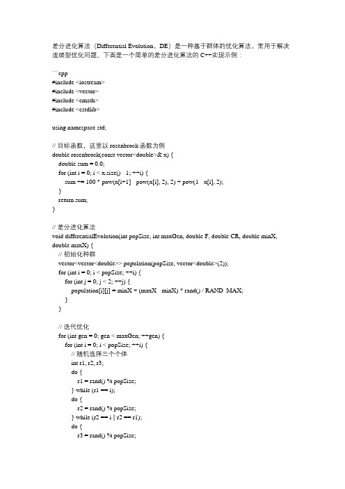
差分进化算法(Differential Evolution,DE)是一种基于群体的优化算法,常用于解决连续型优化问题。下面是一个简单的差分进化算法的C++实现示例:
```cpp #include #include #include #include
using namespace std; // 目标函数,这里以rosenbrock函数为例 double rosenbrock(const vector& x) { double sum = 0.0; for (int i = 0; i < x.size() - 1; ++i) { sum += 100 * pow(x[i+1] - pow(x[i], 2), 2) + pow(1 - x[i], 2); } return sum; }
// 差分进化算法 void differentialEvolution(int popSize, int maxGen, double F, double CR, double minX, double maxX) { // 初始化种群 vector> population(popSize, vector(2)); for (int i = 0; i < popSize; ++i) { for (int j = 0; j < 2; ++j) { population[i][j] = minX + (maxX - minX) * rand() / RAND_MAX; } }
// 迭代优化 for (int gen = 0; gen < maxGen; ++gen) { for (int i = 0; i < popSize; ++i) { // 随机选择三个个体 int r1, r2, r3; do { r1 = rand() % popSize; } while (r1 == i); do { r2 = rand() % popSize; } while (r2 == i || r2 == r1); do { r3 = rand() % popSize; } while (r3 == i || r3 == r1 || r3 == r2); // 变异操作 vector trial(population[i].size()); for (int j = 0; j < trial.size(); ++j) { trial[j] = population[r1][j] + F * (population[r2][j] - population[r3][j]); }
差分进化算法原理

差分进化算法原理差分进化算法是一种基于群体智能的优化算法,由Storn和Price于1995年提出。
该算法通过模拟生物遗传进化的过程,在群体中引入变异、交叉、选择等操作,从而优化目标函数。
相对于传统优化算法,差分进化算法具有收敛速度快、全局搜索能力强等优点,因此在实际工程优化中得到广泛应用。
差分进化算法的基本原理是通过不断改进目标函数来优化群体中的个体。
算法的基本流程如下:1. 初始化:随机生成足够多的初始个体,构成初始群体。
2. 变异:对于每个个体,根据固定的变异策略生成一个变异个体。
3. 交叉:将原个体和变异个体进行交叉,得到一个新的个体。
4. 选择:从原个体和交叉个体中选择更优的一个作为下一代的个体。
5. 更新群体:将新个体代替原个体,同时保留所有代的最优解。
变异策略和交叉方法是差分进化算法的核心部分。
1. 变异策略:变异策略是指在进化过程中,对每个个体进行的变异操作。
常用的变异策略有DE/rand/1、DE/rand/2和DE/best/1等。
“DE”表示差分进化,“rand”表示随机选择其他个体进行变异,“best”表示选择当前代的最优解。
以DE/rand/1为例,其变异操作步骤如下:(1)从群体中随机选择两个个体(除当前个体之外);(2)根据固定的变异因子F,生成一个变异向量v;(3)计算原个体与变异向量v的差分,得到新的个体。
变异因子F的值通常取0.5-1.0,表示变异向量中各项的取值在变量取值范围内随机变化的程度。
2. 交叉方法:交叉方法是指在变异个体和原个体之间进行的交叉操作。
常用的交叉方法有“二项式交叉”和“指数交叉”等。
以二项式交叉为例,其交叉操作步骤如下:(1)对于变异向量v中的每一维,以一定的概率Cr选择变异向量中的该维,否则选择原个体中的该维;(2)得到新的个体。
Cr表示交叉率,通常取值在0.1-0.9之间。
差分进化算法的收敛性和全局搜索能力与变异策略和交叉方法的选择密切相关。
老陈汽车英语 词组
老陈汽车英语词组Electrical system电器系统internal combustion engine内燃发动机fuel system燃料系统exhaust system排气系统cooling system冷却系统lubrication system润滑系统ignition system点火系统air-fuel system可燃混合气体power stroke工作冲程power train传动系统suspension system悬架系统steering system转向系统brake system制动系统propeller shaft传动系统rear axle后桥steering wheel方向盘steering shaft转向轴gear sector扇形齿轮pitman arm转向摇臂drag link直拉杆steering knuckle arm转向节臂king pin主销steering arm转向臂tie rod转向横拉杆front axle前轴steering knuckle arm转向节臂steering knuckle转向节by means of依靠brake drum制动鼓brake shoe制动蹄片brake lining制动衬片service brake行车制动器parking brake驻车制动roof panel顶板instrument panel仪表板luggage compartment行李间karl benz卡尔本次apply for申请by leaps and bounds非常迅速的set out出发开始henry ford亨利福特assemble line装配线ford福特Lincoln林肯American general motors通用Buick别克Chevrolet雪佛兰Oldsmobile奥兹莫比尔Cadillac凯迪拉克Chrysler克莱斯勒Plymouth普利茅斯In essential实质上Toyota丰田Nissan尼桑Driving license驾照No。
- 1、下载文档前请自行甄别文档内容的完整性,平台不提供额外的编辑、内容补充、找答案等附加服务。
- 2、"仅部分预览"的文档,不可在线预览部分如存在完整性等问题,可反馈申请退款(可完整预览的文档不适用该条件!)。
- 3、如文档侵犯您的权益,请联系客服反馈,我们会尽快为您处理(人工客服工作时间:9:00-18:30)。
Differential evolution with hybrid linkagecrossoverYiqiao Cai a ,⇑,Jiahai Wang baCollege of Computer Science and Technology,Huaqiao University,Xiamen 361021,China b Department of Computer Science,Sun Yat-sen University,Guangzhou 510006,Chinaa r t i c l e i n f o Article history:Received 2March 2014Received in revised form 5February 2015Accepted 15May 2015Available online 27May 2015Keywords:Differential evolution Linkage learning Crossover Grouping Numerical optimizationa b s t r a c tIn the field of evolutionary algorithms (EAs),differential evolution (DE)has been the sub-ject of much attention due to its strong global optimization capability and simple imple-mentation.However,in most DE algorithms,crossover operator often ignores theconsideration of interactions between pairs of variables.That is,DE is linkage-blind,andthe problem-specific linkages are not utilized effectively to guide the search process.Furthermore,linkage learning techniques have been verified to play an important role inEA optimization.Therefore,to alleviate the drawback of linkage-blind in DE and enhanceits performance,a novel linkage utilization technique,called hybrid linkage crossover(HLX),is proposed in this study.HLX utilizes the perturbation-based method to automat-ically extract the linkage information of a specific problem and then uses the linkage infor-mation to guide the crossover process.By incorporating HLX into DE,the resultingalgorithm,named HLXDE,is presented.In order to evaluate the effectiveness of HLXDE,HLX is incorporated into six original DE algorithms,as well as several advanced DE vari-ants.Experimental results demonstrate the high performance of HLX for the DE algorithmsstudied.Ó2015Elsevier Inc.All rights reserved.1.IntroductionDifferential evolution (DE),proposed by Storn and Price [55],is a simple and powerful evolutionary algorithm (EA)for global optimization over continuous space.In the field of EA,DE has been the subject of much attention due to its attractive characteristics,such as its compact structure,ease of use,speediness and robustness.In the last few years,DE has been extended for handling multiobjective,constrained,large scale,dynamic and uncertain optimization problems [11,40]and is now successfully used in various scientific and engineering fields [47,66,19,85],such as chemical engineering,engineering design,and pattern recognition.When DE is applied to a given optimization problem,there are two main factors which significantly affect the behavior of DE:control parameters (i.e.,population size NP ,mutation scaling factor F and crossover rate Cr )and evolutionary operators (i.e.,mutation,crossover and selection).During the last decade,many researchers have worked to improve DE by adopting self-adaptive strategies for the control parameters [48,30,13],devising new mutation operators [23,5,67],developing ensem-ble strategies [68,25,6],and proposing a hybrid DE with other optimization algorithms [73,46,64],etc.Many studies related to the evolutionary operators of DE have focused on the mutation operator [48,30,23,5,68,25].In contrast,there have been few studies on the crossover operator of DE [43,24,69]./10.1016/j.ins.2015.05.0260020-0255/Ó2015Elsevier Inc.All rights reserved.⇑Corresponding author.E-mail addresses:caiyq@ (Y.Cai),wjiahai@ (J.Wang).Y.Cai,J.Wang/Information Sciences320(2015)244–287245 Linkages or inter-dependencies between pairs of variables have been studied and utilized in genetic algorithm(GA)and EAs to improve performance on difficult problems[8,65].From the perspective of GA,tight linkage refers to the identified building blocks(BBs)on a chromosome,and the genes belonging to the same BB should be inherited together by the off-spring at a higher probability.According to the existing work,linkage identification or recognition of BBs plays an important role in GA optimization[8,65].Many linkage learning techniques have been proposed for combinatorial optimization [8,65,17],while techniques for global numerical optimization have been rarely discussed[84,7].In addition,to the best of our knowledge,studies explicitly using linkage information to enhance the performance of DE are scarce.Therefore,most DE algorithms are not able to effectively utilize problem-specific linkages for guiding the search.Based on these considerations,we present a novel linkage utilization technique,called hybrid linkage crossover(HLX),to utilize the problem-specific linkages to guide the crossover process of DE.First,HLX uses a perturbation-based method,an improved differential grouping(DG)method[44],to adaptively extract the linkage information between pairs of variables. The linkage information is stored in a linkage matrix(LM).In LM,each element stands for‘‘linkage strength’’which measures the likelihood of a pair of variables being tightly linked.Then,with LM,the BBs are identified by automatically decomposing the problem variables into different groups without overlaps.Here,BB is a group of tightly interactive variables.Finally,two group-wise crossover operators are designed to explicitly use the identified BBs for guiding the crossover process.One is named group-wise binomial crossover(GbinX).Different from the conventional binomial crossover of DE,GbinX exchanges the variables based on the detected groups.The second one is referred to as group-wise orthogonal crossover(GorthX), which combines the orthogonal design[27,38]and the identified BBs to make a systematic search in a region defined by a pair of the target and mutant vectors.In this way,both GbinX and GorthX can avoid the disruption of BBs during crossover. By incorporating HLX into DE,the resulting algorithm,named HLXDE,is proposed.In HLXDE,the conventional binomial crossover operator and the two group-wise crossover operators are implemented together in a cooperative manner.In order to evaluate the effectiveness of HLXDE,HLX is incorporated into six original DE algorithms,as well as several advanced DE variants.Experimental studies are carried out on a suite of benchmark problems,including the classical func-tions[74],the functions from the IEEE congress on evolutionary computation(CEC)2005special session on real-parameter optimization[56]and the functions from the IEEE CEC2012special session on large-scale global optimization[60].The results indicate that HLX can effectively enhance the performance of most DE algorithms studied.The major contributions of this study include the following:An improved differential grouping technique is presented to address the linkage learning problem for global numer-ical optimization.It provides some insights on how the idea of grouping variables can be extended beyond the coop-erative coevolution framework.Two group-wise crossover operators,GbinX and GorthX,are designed to explicitly utilize the identified BBs to guide the crossover process of DE.HLXDE effectively combines two group-wise crossover operators with the binomial crossover in a cooperative man-ner,which effectively maintains the advantages of the binomial crossover and utilizes the BBs of good or promising individuals.HLX can be easily applied to other advanced DE variants and cooperated with different kinds of modifications in the advanced DE variants.It provides a new promising approach for optimization.The rest of this paper is organized as follows.Section2briefly describes the original DE algorithm,the related work to the crossover operator of DE and the linkage learning techniques.Then,HLX and HLXDE are presented in detail in Section3.In Section4,the experimental results for a suite of benchmark functions are reported and analyzed.Finally,the conclusions are drawn in Section5.2.Related workIn this section,the original DE algorithm is introducedfirst.Then,the related work to the crossover operator of DE and the linkage learning techniques are reviewed.2.1.DEDE is for solving the numerical optimization problem.Without loss of generality,we consider the following optimization problem:Minimize fðXÞ;X2S,where S#R D and D is the dimension of the decision variables.DE evolves a population of vec-tors,and each vector is denoted as X i;G¼ðx1;i;G;x2;i;G;...;x D;i;GÞ,where i¼1;2;...;NP;NP is the size of the population and G is the number of current iteration.Here,the initial value of the j th parameter of X i;G can be generated by:x j;i;G¼L jþrndrealð0;1ÞÁðU jÀL jÞð1Þwhere rndrealð0;1Þrepresents a uniformly distributed random variable within the range[0,1]and L j(U j)represents the lower(upper)bound of the j th variable.During each generation,DE uses three main operators for population reproduction:mutation,crossover and selection.(1)Mutation:DE employs the mutation strategy to generate a mutant vector V i;G with respect to each individual X i;G (called the target vector)in the current population.The general notation for mutation strategy is‘‘DE/x/y’’,where DE stands for differential evolution algorithm,x represents the vector to be perturbed and y represents the number of difference vec-tors considered for perturbation of x.Two commonly used strategies are as follows:‘‘DE/rand/1’’V i;G¼X r1;GþFÁðX r2;GÀX r3;GÞð2Þ ‘‘DE/best/1’’V i;G¼X best;GþFÁðX r2;GÀX r3;GÞð3Þwhere F is called the mutation scaling factor,and r1;r2and r3are distinct integers randomly selected from the range[1,NP] and are different from i.There are various well-known and widely used mutation strategies in the literature,such as ‘‘DE/rand/2’’,‘‘DE/current-to-best/1’’,‘‘DE/rand-to-best/1’’and‘‘DE/best/2’’.More details of them can be found in[55,11].(2)Crossover:The crossover operator is applied to each pair of X i;G and the corresponding V i;G to generate a trial vector U i;G. There are two types of crossover scheme:binomial and exponential.Here,only the binomial crossover(BinX)is outlined,as it is more widely used.BinX is shown as follows:u j;i;G¼v j;i;G if rndrealð0;1Þ6Cr or j¼jrandx j;i;G otherwiseð4Þwhere Cr2½0;1 is called the crossover rate,and jrandis an integer randomly selected from the range[1,D].In this study,if u j;i;G is out of the boundary,it will be reinitialized within the range[L j;U j].(3)Selection:DE uses a one-to-one selection operator to select the better one between X i;G and U i;G to survive into the next generation.The selection operator is described as follows:X i;Gþ1¼U i;G if fðU i;GÞ6fðX i;GÞX i;G otherwiseð5Þ2.2.Crossover operator in DEDE has drawn many researchers’attention,which has resulted in many variants with improved performance[11,41]. According to[41],these DE variants can be divided into two categories:DE with an extra component and DE with modified structures.In the existing work of DE,the mutation operator has been studied in various ways.In contrast,there are few studies on the crossover operator of DE[11,41].In this section,we focus on the work related to the crossover operator in the context of DE.Table1provides a list of some previous studies on the crossover operator in DE along with different facets (i.e.,tuning Cr value,parameter adaption technique and crossover scheme).Many researchers focus on tuning Cr to improve the performance of DE.From Table1,we canfind that these empirical suggestions for setting Cr are different and lack sufficient experimental justifications.However,some interesting observa-tions can be obtained from thesefindings.A small Cr value(e.g.,Cr60:2)is more appropriate for the separable functions, and a large Cr value(e.g.,Cr>0:9)is the best for non-separable functions.For the role of Cr in optimizing functions with interacting parameters,the greater the number of interacting parameters,the higher Cr must be.In addition,from the anal-ysis in[39],DE with low values of Cr(near0)results in very small exploratory moves that are orthogonal to the current axes, while DE with high values of Cr(near1)makes large exploratory moves that are at angles to the search space’s axes.That is, both extremes are able to produce effective moves[39].In order to avoid manual tuning Cr,many parameter adaption tech-niques have been developed[48,30,33,80,4,34,79,61,31].These researches presented the effective methods to adaptively tune the Cr value.On the other hand,from Table1,we can see that the studies on the new crossover scheme in DE are relatively few.In most of the DE variants,BinX is employed as the default.As mentioned above,the crossover operator has always been regarded as the primary search operator in GA,and the linkage identification or recognizing BBs plays an important role in the GA opti-mization[8,65].However,in most of the crossover operators of DE,the linkage information is not effectively identified and used to enhance the performance of DE.Based on these analyses,in this study,we develop HLX to utilize the problem-specific linkages to guide the crossover process of DE.2.3.Linkage learningIn GA and EAs,the identification and preservation of important interactions among variables have a desirable effect on the evolutionary process,which is generally called linkage learning.In biological systems,linkage refers to the level of asso-ciation in inheritance of two or more non-allelic genes on the same chromosome[28].These linked genes have a higher chance of being inherited from the same parent.In GA,linkage is used to describe and measure the interrelationships 246Y.Cai,J.Wang/Information Sciences320(2015)244–287Y.Cai,J.Wang/Information Sciences320(2015)244–287247Table1Previous studies on crossover operator in DE.Taxonomy Reference work ApproachesTuning Cr Storn and Price[55]Cr could be set to0.1or0.9to obtain good performanceMezura-Montes et al.[36]A low value of Cr¼0:1was often the best chosenRon¨kkon¨en et al.[50]Cr60:2was more appropriate for the separable functions and Cr close to1.0(e.g.,Cr>0:9)was the best for non-separable functionsMontgomery and Chen[39]DE behaved differently with low and high values of Cr and both extremes areable to produce effective movesParameter adaption technique Qin et al.[48],Zhang et al.[83]Cr was gradually self-adapted by learning from their previous experiences ingenerating promising solutionsLiu and Lampinen[33]Fuzzy logic controllers were used to adapt the Cr valueZaharie[80]Adaptive control was based on the idea of controlling the population diversityBrest et al.[4]Self-adaptive settings by extending individuals with the Cr valueMallipenddi et al.[34]A pool of Cr values was taken in the range of0.1–0.9Yu et al.[79]Two-level adaptive parameter control scheme based on the optimization statesand the individual’sfitness valueTang et al.[61]Individual-dependent parameter setting with a rank-based scheme and a value-based schemeCrossover scheme Storn and Price[55]Two kinds of well-known crossover schemes,binomial and exponentialcrossoverZaharie[81]A systematic analysis of the influence of binomial and exponential crossover onthe behavior of DEZhao et al.[86]A linearly scalable exponential crossover operator based on a number ofconsecutive dimensions to crossoverWeber and Neri[71]A contiguous binomial crossover with the exchange of contiguous block in afashion similar to the exponential crossoverLin et al.[32]The choice of crossover method and parameters were related to themathematical features of the problemsGou et al.[26]Eigenvector-based crossover operator by utilizing eigenvectors of covariancematrix of individual solutionsNoman and Iba[43]A simplex crossover-based adaptive local search operatorGong et al.[24],Wang et al.[69]An orthogonal crossover combined with the conventional crossoverexisting between the genes.These highly interactive genes belong to a BB.When GA is applied to a given optimization prob-lem,Holland[29]suggested that the genes belonging to the same BB should be tightly linked together on the chromosome to improve performance.Otherwise,if these linked genes spread all over the chromosome,the BBs are very hard to create and are easy to be disrupted during crossover,for example,single-point crossover.This suggestion is also supported in some studies[8,21,62].Furthermore,for the continuous optimization,Chen et al.[7]suggested that the crossover with dynamic linkage technique is beneficial to utilizing the obtained linkage information.Therefore,identifying or recognizing BBs plays an important role in crossover of GA and EAs.However,it is often difficult to know the linkage information of a specific prob-lem in the real world a priori.As a consequence,linkage learning has been studied in both the discrete and continuous GA and EAs[8,65,7,12,63].Table2provides a list of some previous studies on linkage learning for discrete and continuous opti-mization problems.For the discrete optimization problems,there are many linkage learning techniques proposed to improve the performance of GA and EAs.From Table2,these linkage learning techniques can be classified into three categories based on different aspects of GA and EAs:how to distinguish between the good and bad linkages,how to express or represent linkage informa-tion and how to store linkage information[8].More details of other linkage learning techniques in GA and EAs can be found in[8].For the continuous optimization problems,linkage learning has been studied less.As shown in Table2,there are several linkage learning methods for continuous optimization,such as dynamic linkage discovery[7],estimation of dis-tribution algorithms(EDAs)[84],perturbation-based methods(PMs)[12,44]and data mining techniques[63].In dynamic linkage discovery,the linkage configuration is adapted by assigning the linkage groups randomly[7]. Hence,dynamic linkage discovery does not rely on a systematic or smart procedure to discover the interactions among variables.It may happen that the problem-specific BBs are very hard to create and are destroyed easily during the crossover process.While identifying linkage in a statistical manner,EDAs generally tend to ignore BBs with a relatively lowfitness contribution[9,63],and the computational cost of them is usually very high,for example,the Bayesian optimization algorithm(BOA)[45].Recently,in the context of PMs for continuous global optimization,differential grouping(DG)which is an automatic decomposition strategy,was superimposed on a cooperative co-evolutionary framework in[44].Based on the above analysis and the effectiveness of DG,a new linkage utilization technique based on DG is developed for the continuous optimization problems in this study.3.Differential evolution with hybrid linkage crossover(HLXDE)3.1.MotivationAs discussed above,the crossover operator plays an important role in the performance of DE[81,86,71,32,43,24,69]. The existing work[8,65,7,9,12]also demonstrates that the crossover with linkage learning can effectively prevent the linkages between pairs of variables from being destroyed and promote the cooperation of individuals of population. In most DE algorithms,BinX(see Eq.(4))is employed to generate a trial vector from a pair of target and mutant vectors. As we canfind,each variable of the trial vector in BinX is randomly and independently inherited from either target vec-tor or mutant vector based on Cr.In this way,the linkage information between pairs of variables is ignored during the crossover process.That is,DE is linkage-blind,and thus the problem-specific linkages cannot be utilized to guide the evolutionary process.As discussed in[39,86,81,58],although DE can solve the non-separable functions with a high value of Cr,DE with a high Cr value will cause rapid and perhaps premature convergence unless the population size is large enough.In addition,DE with high values of Cr will take a longer time to solve these non-separable functions than that with low values of Cr[39].That is,DE has difficulty on functions that are not linearly separable,and the linkage learning techniques might be used to further improve the performance of DE on these functions.Therefore,in order to alleviate this drawback and utilize the problem-specific linkages for enhancing the performance of DE,we propose HLX and then incorporate it into DE to present HLXDE in this study.The details of HLX and the complete framework of HLXDE are described as follows.3.2.HLXFor many problems,the problem-specific knowledge does not exist in the individual variables but in the linkages between pairs of variables.In order to detect the underlying interaction structure of these variables and to guide the crossover process with the problem-specific linkage,HLX consists of three main operators:(1)constructing the linkage matrix to extract and store the linkage information;(2)adaptively grouping the problem variables to detect BBs;(3)applying group-wise cross-over to explicitly use BBs for guiding the crossover process.Algorithm1.Linkage Matrix Construction(LMC)1:Initialize a vector C0¼ðc01;...;c0i;...;c0DÞand set c0ias lbound i;i¼1;...;D2:Initialize D max¼0//calculate difference value of pair variables3:For i¼1to DÀ1do4:Set c0ias ubound i and name the new vector as C15:Calculate D1;xi½f ðXÞ¼fðC1ÞÀfðC0Þ6:For j¼iþ1to D do7:Set c1jas midbound j and name the new vector as C28:Set c2ias lbound j and name the new vector as C39:Calculate D2;xi½f ðXÞ¼fðC2ÞÀfðC3Þ10:Calculate D xi ;x j½f ðXÞusing Eq.(8)11:If j D xi ;x j½f ðXÞj<fðC0ÞÂ10À3Then12:Set D xi ;x j½f ðXÞ¼013:End if14:If j D xi ;x j½f ðXÞj>D max Then15:Set D max¼D xi ;x j½f ðXÞ16:End if17:End for18:End for//normalize difference values and store them in LM19:For i¼1to D do20:For j¼1to D do21:calculate LM½i;j using Eq.(9)22:End For23:End For248Y.Cai,J.Wang/Information Sciences320(2015)244–2873.2.1.Linkage matrix construction (LMC)By detecting the fitness changes from perturbing pairs of variables,the perturbation-based methods are employed to identify the interactive variables.Recently,differential grouping (DG)has been proposed to decompose the problem auto-matically,deriving from the definition of partial separability [44].Due to its theoretical basis and effectiveness,DG is adopted and improved in HLX to detect the underlying structure of a specific problem.With the linkage information obtained by the improved DG,a linkage matrix (LM )is constructed to explicitly represent the linkage information between pairs of variables.Given a function f ðx Þ,two difference values with respect to variable x i are calculated as follows [44]:D d ;x i ½f ðX Þj x i ¼a ;x j ¼b ¼f ð...;x i À1;a þd ;x i þ1;...;x j À1;b ;x j þ1;...ÞÀf ð...;x i À1;a ;x i þ1;...;x j À1;b ;x j þ1;...Þð6ÞD d ;x i ½f ðX Þj x i ¼a ;x j ¼c ¼f ð...;x i À1;a þd ;x i þ1;...;x j À1;c ;x j þ1;...ÞÀf ð...;x i À1;a ;x i þ1;...;x j À1;c ;x j þ1;...Þð7Þwhere a is an arbitrary value for x i ;d –0is a nonzero interval value,and b and c are two arbitrary different values for x j .In Eqs.(6)and (7),D d ;x i ½f ðX Þj x i ¼a ;x j ¼b and D d ;x i ½f ðX Þj x i ¼a ;x j ¼c refer to the forward difference of f ðx Þwith respect to x i with d .Then,the difference value between them is calculated as follows:D x i ;x j ½f ðX Þ¼D d ;x i ½f ðX Þj x i ¼a ;x j ¼b ÀD d ;x i ½f ðX Þj x i ¼a ;x j ¼cð8ÞAfter that,the difference value of each pair of variables is normalized and stored in LM ,as follows:LM ½i ;j ¼D x i ;x j ½f ðX Þmax ð9Þwhere D max is the maximum value in LM .If LM ½i ;j is zero,x i and x j are regarded to be independent of each other or separable.Otherwise,they will be considered to be interacting or non-separable.In this way,LM construction (LMC)operator extracts and stores the linkage information between pairs of variables in LM .Each element of LM stands for ‘‘linkage strength’’,which measures the likelihood of a pair of variables being tightly linked.The pseudo-code of LMC is described in Algorithm 1where lbound i ;ubound i and midbound i represent the lower,upper and center bound of x i respectively.Note that these values can be set randomly as long as they are not identical with each otherTable 2Previous studies on linkage learning in discrete and continuous optimization problems.TaxonomyReference work Approaches Discrete optimization problems Salman et al.[51–53]The probabilistic inference framework was used for modelingcrossover operators and proposed an adaptive linkagecrossoverGoldberg et al.[20,22],Bandyopadhyay et al.[3]Messy genetic algorithm (mGA)was proposed to solveproblems by combining relatively short and well-testedbuilding blocks to form longer and more complexsubstructuresEmmendorfer and Pozo [14]A simple EDA based on low-order statistic and a clusteringtechnique was combined to propose a new evolutionaryalgorithm,u -PBILYu et al.[75–78]A dependency structure matrix GA (DSMGA)was proposedby utilizing a dependency structure matrix (DSM)to analyzeand explicitly decompose the problem and using the BBsinformation to accomplish crossoverFan et al.[17,16],Nikanjam et al.[42]Improved variants were proposed to enhance theperformance of DSMGAContinuous optimization problems Chen et al.[7]Dynamic linkage discovery was proposed to adapt thelinkage configuration by employing the selection operatorwithout extra judging criteria irrelevant to the objectivefunctionZhange et al.[84]A regularity model-based multiobjective estimation ofdistribution algorithm (RM-MEDA)for continuousmultiobjective optimization problems with variable linkagesDevicharan and Mohan [12]Problem specific linkages was learned by examining arandomly chosen collection of points in the search space todetermine the correlations in fitness changes resulting fromperturbations in pairs of components of particle positionsOmidvar et al.[44]Differential grouping was proposed to automaticallydecompose an optimization problem into a set of smallerproblems for large scale optimizationTing et al.[63]Linkage was mined based on the analogy between buildingblocks and association rules Y.Cai,J.Wang /Information Sciences 320(2015)244–287249so as to obtain the nonzero difference value.Additionally,if the difference value between x i and x j is smaller than f ðC 0ÞÂ10À3,they are regarded to be independent of each other in this study (see steps 11–13in Algorithm 1).In order to illustrate how LMC works,a simple example based on Noisy Quartic function at D ¼8is shown here.The def-inition of Noisy Quartic function is as follows [74]:f ðX Þ¼X 8i ¼1ix 4i þrandom ½0;1Þ;À1:286x i 61:28ð10ÞFirstly,a vector is initialized as C 0¼ðÀ1:28;...;À1:28Þand the difference values for pairs of variables are calculated using Eq.(8)(Here,a ¼b ¼À1:28;d ¼2Ã1:28¼2:56;c ¼0),as follows:D x 1;x 2½f ðX Þ¼ðf ð1:28;À1:28;...;À1:28ÞÀf ðC 0ÞÞÀðf ð1:28;0;À1:28;...;À1:28ÞÀf ðÀ1:28;0;À1:28;...;À1:28ÞÞD x 1;x 3½f ðX Þ¼ðf ð1:28;À1:28;...;À1:28ÞÀf ðC 0ÞÞÀðf ð1:28;À1:28;0;À1:28;...;À1:28ÞÀf ðÀ1:28;À1:28;0;À1:28;...;À1:28ÞÞÁÁÁD x 7;x 8½f ðX Þ¼ðf ðÀ1:28;...;À1:28;1:28;À1:28ÞÀf ðC 0ÞÞÀðf ðÀ1:28;...;À1:28;1:28;0ÞÀf ðÀ1:28;...;À1:28;À1:28;0ÞÞSecondly,a difference matrix (DM )is used to store all the difference values,as follows:0:001:210:320:781:550:780:780:781:210:001:541:541:541:541:611:680:321:540:001:541:541:541:611:680:781:541:540:000:560:560:942:131:551:541:540:560:001:041:041:040:781:541:540:561:040:001:611:680:781:611:610:941:041:610:001:480:781:681:682:131:041:681:480:000B B B B B B B B B B B B B @1C C C C C C C C C C C C C Að11ÞFinally,all the difference values are normalized with D max ¼2:13using Eq.(9),and LM is constructed as follows:0:000:570:150:370:730:370:370:370:570:000:720:720:720:720:760:790:150:720:000:720:720:720:760:790:370:720:720:000:260:260:441:000:730:720:720:260:000:490:490:490:370:720:720:260:490:000:760:790:370:760:760:440:490:760:000:690:370:790:791:000:490:790:690:000B B B B B B B B B B B B B @1C C C C C C C C C C C C C A ð12Þ3.2.2.Adaptive grouping (AG)After LMC,BBs are identified by AG to decompose the variables of a problem into different groups without overlap.Here,BB is a group of highly interactive variables.The pseudo-code of AG is described in Algorithm 2where a state vector (i.e.,Z )is used to examine whether the variable has been grouped.The algorithm starts by checking the linkage strength of the first variable with other variables based on LM .If the state value of the j th variable (j ¼2;3;...;D )is marked as not being grouped (i.e.,z j ¼0)and LM ½1;j is greater than a threshold value ( ),the j th variable is placed into the same group with the first vari-able and its state value is changed to 1(i.e.,z j ¼1).This process is repeated until all the variables are grouped.In this study, is adaptively set as the mean value of all the elements in LM ,which is shown in step 2of Algorithm 2.Additionally,in order to enhance the search ability of HLX,grouping is not carried out in sequential order but in a random order p .That is,let p ði Þbe a random permutation of i ¼1;2;...;D and grouping is carried out following the order given by the permutation p ði Þ.Although employing a similar way of detecting the interaction between pairs of variables,AG has some differences from DG [44].First,as discussed in [44],without prior knowledge about the problem,the decomposition with a specified thresh-old value is not effective for all the problems,and how to set the threshold value is still a difficult problem.In DG,the thresh-old value is pre-set,while the threshold value ( )in AG is set adaptively for different problems.The effectiveness of adaptive value will be studied in Section 4.7.Second,grouping in AG is carried out based on LM .In LM ,each element represents the linkage strength between a pair of variables.In addition,randomness is also introduced into AG to generate different250Y.Cai,J.Wang /Information Sciences 320(2015)244–287。