A Simplicial Approach for Discrete Fixed Point Theorems (Extended Abstract)
The NASA STI Program Office... in Profile

NASA/CR-2002-211768
Very Large Scale Optimization
Garrett Vanderplaats Vanderplaats Research and Development, Inc., Colorado Springs, Colorado
National Aeronautics and Space Administration Langley Research Center Hampton, Virginia 23681-2199 Prepared for Langley Research Center under Contract NAS1-00102
TECHNICAL TRANSLATION. Englishlanguage translations of foreign scientific and technical material pertinent to NASA’s mission.
Specialized services that complement the STI Program Office’s diverse offerings include creating custom thesauri, building customized databases, organizing and publishing research results . . . even providing videos. For more information about the NASA STI Program Office, see the following: • Access the NASA STI Program Home Page at • Email your question via the Internet to help@ • Fax your question to the NASA STI Help Desk at (301) 621-0134 • Telephone the NASA STI Help Desk at (301) 621-0390 • Write to: NASA STI Help Desk NASA Center for AeroSpace Information 7121 Standard Drive Hanover, MD 21076-1320
中医骨科学外文版10

Advantages of small splint fixation
(1) Non-invasive fixation: It causes no damage to limb tissues and can be used for fixation of limb fractures in the elderly, children, and patients not suitable for surgical treatment.
Fixation standard
No damage to the surrounding soft tissue, normal blood supply at the injured site, and no obstruction to normal healing
Eliminate various unfavorable factors for fracture healing, stabilize the fracture end, and create favorable conditions for healing
Indications of small splint fixation
On-site first aid
Байду номын сангаас
Indications of small splint fixation
Fixation of closed limb fracture after reduction
(1) It exhibits a better fixation effect for stable fractures at the long bone of the upper extremity and tibial and fibular shafts.
chapter_2
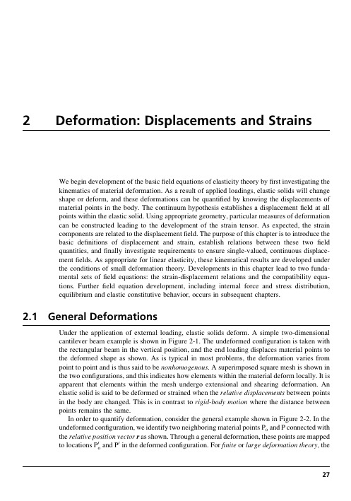
2Deformation:Displacements and Strains We begin development of the basicfield equations of elasticity theory byfirst investigating thekinematics of material deformation.As a result of applied loadings,elastic solids will changeshape or deform,and these deformations can be quantified by knowing the displacements ofmaterial points in the body.The continuum hypothesis establishes a displacementfield at allpoints within the elastic ing appropriate geometry,particular measures of deformationcan be constructed leading to the development of the strain tensor.As expected,the straincomponents are related to the displacementfield.The purpose of this chapter is to introduce thebasic definitions of displacement and strain,establish relations between these twofieldquantities,andfinally investigate requirements to ensure single-valued,continuous displace-mentfields.As appropriate for linear elasticity,these kinematical results are developed underthe conditions of small deformation theory.Developments in this chapter lead to two funda-mental sets offield equations:the strain-displacement relations and the compatibility equa-tions.Furtherfield equation development,including internal force and stress distribution,equilibrium and elastic constitutive behavior,occurs in subsequent chapters.2.1General DeformationsUnder the application of external loading,elastic solids deform.A simple two-dimensionalcantilever beam example is shown in Figure2-1.The undeformed configuration is taken withthe rectangular beam in the vertical position,and the end loading displaces material points tothe deformed shape as shown.As is typical in most problems,the deformation varies frompoint to point and is thus said to be nonhomogenous.A superimposed square mesh is shown inthe two configurations,and this indicates how elements within the material deform locally.It isapparent that elements within the mesh undergo extensional and shearing deformation.Anelastic solid is said to be deformed or strained when the relative displacements between pointsin the body are changed.This is in contrast to rigid-body motion where the distance betweenpoints remains the same.In order to quantify deformation,consider the general example shown in Figure2-2.In the undeformed configuration,we identify two neighboring material points P o and P connected withthe relative position vector r as shown.Through a general deformation,these points are mappedand P0in the deformed configuration.Forfinite or large deformation theory,the to locations P0o27undeformed and deformed configurations can be significantly different,and a distinction between these two configurations must be maintained leading to Lagrangian and Eulerian descriptions;see,for example,Malvern(1969)or Chandrasekharaiah and Debnath(1994). However,since we are developing linear elasticity,which uses only small deformation theory, the distinction between undeformed and deformed configurations can be dropped.Using Cartesian coordinates,define the displacement vectors of points P o and P to be u o and u,respectively.Since P and P o are neighboring points,we can use a Taylor series expansion around point P o to express the components of u asu¼u oþ@u@xr xþ@u@yr yþ@u@zr zv¼v oþ@v@xr xþ@v@yr yþ@v@zr zw¼w oþ@w@xr xþ@w@yr yþ@w@zr z(2:1:1)FIGURE2-1Two-dimensional deformation example.(Undeformed)(Deformed) FIGURE2-2General deformation between two neighboring points.28FOUNDATIONS AND ELEMENTARY APPLICATIONSNote that the higher-order terms of the expansion have been dropped since the components of r are small.The change in the relative position vector r can be written asD r¼r0Àr¼uÀu o(2:1:2) and using(2.1.1)givesD r x¼@u@xr xþ@u@yr yþ@u@zr zD r y¼@v@xr xþ@v@yr yþ@v@zr zD r z¼@w@xr xþ@w@yr yþ@w@zr z(2:1:3)or in index notationD r i¼u i,j r j(2:1:4) The tensor u i,j is called the displacement gradient tensor,and may be written out asu i,j¼@u@x@u@y@u@z@v@x@v@y@v@z@w@x@w@y@w@z2666666437777775(2:1:5)From relation(1.2.10),this tensor can be decomposed into symmetric and antisymmetric parts asu i,j¼e ijþ!ij(2:1:6) wheree ij¼12(u i,jþu j,i)!ij¼12(u i,jÀu j,i)(2:1:7)The tensor e ij is called the strain tensor,while!ij is referred to as the rotation tensor.Relations (2.1.4)and(2.1.6)thus imply that for small deformation theory,the change in the relative position vector between neighboring points can be expressed in terms of a sum of strain and rotation bining relations(2.1.2),(2.1.4),and(2.1.6),and choosing r i¼dx i, we can also write the general result in the formu i¼u o iþe ij dx jþ!ij dx j(2:1:8) Because we are considering a general displacementfield,these results include both strain deformation and rigid-body motion.Recall from Exercise1-14that a dual vector!i canDeformation:Displacements and Strains29be associated with the rotation tensor such that !i ¼À1=2e ijk !jk .Using this definition,it is found that!1¼!32¼12@u 3@x 2À@u 2@x 3 !2¼!13¼12@u 1@x 3À@u 3@x 1 !3¼!21¼12@u 2@x 1À@u 1@x 2 (2:1:9)which can be expressed collectively in vector format as v ¼(1=2)(r Âu ).As is shown in the next section,these components represent rigid-body rotation of material elements about the coordinate axes.These general results indicate that the strain deformation is related to the strain tensor e ij ,which in turn is a related to the displacement gradients.We next pursue a more geometric approach and determine specific connections between the strain tensor components and geometric deformation of material elements.2.2Geometric Construction of Small Deformation TheoryAlthough the previous section developed general relations for small deformation theory,we now wish to establish a more geometrical interpretation of these results.Typically,elasticity variables and equations are field quantities defined at each point in the material continuum.However,particular field equations are often developed by first investigating the behavior of infinitesimal elements (with coordinate boundaries),and then a limiting process is invoked that allows the element to shrink to a point.Thus,consider the common deformational behavior of a rectangular element as shown in Figure 2-3.The usual types of motion include rigid-body rotation and extensional and shearing deformations as illustrated.Rigid-body motion does not contribute to the strain field,and thus also does not affect the stresses.We therefore focus our study primarily on the extensional and shearing deformation.Figure 2-4illustrates the two-dimensional deformation of a rectangular element with original dimensions dx by dy .After deformation,the element takes a rhombus form as shown in the dotted outline.The displacements of various corner reference points areindicated(Rigid Body Rotation)(Undeformed Element)(Horizontal Extension)(Vertical Extension)(Shearing Deformation)FIGURE 2-3Typical deformations of a rectangular element.30FOUNDATIONS AND ELEMENTARY APPLICATIONSin the figure.Reference point A is taken at location (x,y ),and the displacement components of this point are thus u (x,y )and v (x,y ).The corresponding displacements of point B are u (x þdx ,y )and v (x þdx ,y ),and the displacements of the other corner points are defined in an analogous manner.According to small deformation theory,u (x þdx ,y )%u (x ,y )þ(@u =@x )dx ,with similar expansions for all other terms.The normal or extensional strain component in a direction n is defined as the change in length per unit length of fibers oriented in the n -direction.Normal strain is positive if fibers increase in length and negative if the fiber is shortened.In Figure 2-4,the normal strain in the x direction can thus be defined bye x ¼A 0B 0ÀAB From the geometry in Figure 2-4,A 0B 0¼ffiffiffiffiffiffiffiffiffiffiffiffiffiffiffiffiffiffiffiffiffiffiffiffiffiffiffiffiffiffiffiffiffiffiffiffiffiffiffiffiffiffiffiffiffiffiffiffiffiffiffiffiffidx þ@u @x dx 2þ@v @x dx 2s ¼ffiffiffiffiffiffiffiffiffiffiffiffiffiffiffiffiffiffiffiffiffiffiffiffiffiffiffiffiffiffiffiffiffiffiffiffiffiffiffiffiffiffiffiffiffiffiffiffiffiffiffiffiffiffiffiffiffiffiffi1þ2@u @x þ@u @x 2þ@v @x 2dx s %1þ@u @xdx where,consistent with small deformation theory,we have dropped the higher-order ing these results and the fact that AB ¼dx ,the normal strain in the x -direction reduces toe x ¼@u@x (2:2:1)In similar fashion,the normal strain in the y -direction becomese y ¼@v@y (2:2:2)A second type of strain is shearing deformation,which involves angles changes (see Figure 2-3).Shear strain is defined as the change in angle between two originally orthogonalx FIGURE 2-4Two-dimensional geometric strain deformation.Deformation:Displacements and Strains 31directions in the continuum material.This definition is actually referred to as the engineering shear strain.Theory of elasticity applications generally use a tensor formalism that requires a shear strain definition corresponding to one-half the angle change between orthogonal axes; see previous relation(2:1:7)1.Measured in radians,shear strain is positive if the right angle between the positive directions of the two axes decreases.Thus,the sign of the shear strain depends on the coordinate system.In Figure2-4,the engineering shear strain with respect to the x-and y-directions can be defined asg xy¼p2ÀffC0A0B0¼aþbFor small deformations,a%tan a and b%tan b,and the shear strain can then be expressed asg xy¼@v@xdxdxþ@u@xdxþ@u@ydydyþ@v@ydy¼@u@yþ@v@x(2:2:3)where we have again neglected higher-order terms in the displacement gradients.Note that each derivative term is positive if lines AB and AC rotate inward as shown in thefigure.By simple interchange of x and y and u and v,it is apparent that g xy¼g yx.By considering similar behaviors in the y-z and x-z planes,these results can be easily extended to the general three-dimensional case,giving the results:e x¼@u@x,e y¼@v@y,e z¼@w@zg xy¼@u@yþ@v@x,g yz¼@v@zþ@w@y,g zx¼@w@xþ@u@z(2:2:4)Thus,we define three normal and three shearing strain components leading to a total of six independent components that completely describe small deformation theory.This set of equations is normally referred to as the strain-displacement relations.However,these results are written in terms of the engineering strain components,and tensorial elasticity theory prefers to use the strain tensor e ij defined by(2:1:7)1.This represents only a minor change because the normal strains are identical and shearing strains differ by a factor of one-half;for example,e11¼e x¼e x and e12¼e xy¼1=2g xy,and so forth.Therefore,using the strain tensor e ij,the strain-displacement relations can be expressed in component form ase x¼@u@x,e y¼@v@y,e z¼@w@ze xy¼1@uþ@v,e yz¼1@vþ@w,e zx¼1@wþ@u(2:2:5)Using the more compact tensor notation,these relations are written ase ij¼12(u i,jþu j,i)(2:2:6)32FOUNDATIONS AND ELEMENTARY APPLICATIONSwhile in direct vector/matrix notation as the form reads:e¼12r uþ(r u)TÂÃ(2:2:7)where e is the strain matrix and r u is the displacement gradient matrix and(r u)T is its transpose.The strain is a symmetric second-order tensor(e ij¼e ji)and is commonly written in matrix format:e¼[e]¼e x e xy e xze xy e y e yze xz e yz e z2435(2:2:8)Before we conclude this geometric presentation,consider the rigid-body rotation of our two-dimensional element in the x-y plane,as shown in Figure2-5.If the element is rotated through a small rigid-body angular displacement about the z-axis,using the bottom element edge,the rotation angle is determined as@v=@x,while using the left edge,the angle is given byÀ@u=@y. These two expressions are of course the same;that is,@v=@x¼À@u=@y and note that this would imply e xy¼0.The rotation can then be expressed as!z¼[(@v=@x)À(@u=@y)]=2, which matches with the expression given earlier in(2:1:9)3.The other components of rotation follow in an analogous manner.Relations for the constant rotation!z can be integrated to give the result:u*¼u oÀ!z yv*¼v oþ!z x(2:2:9)where u o and v o are arbitrary constant translations in the x-and y-directions.This result then specifies the general form of the displacementfield for two-dimensional rigid-body motion.We can easily verify that the displacementfield given by(2.2.9)yields zero strain.xFIGURE2-5Two-dimensional rigid-body rotation.Deformation:Displacements and Strains33For the three-dimensional case,the most general form of rigid-body displacement can beexpressed asu*¼u oÀ!z yþ!y zv*¼v oÀ!x zþ!z xw*¼w oÀ!y xþ!x y(2:2:10)As shown later,integrating the strain-displacement relations to determine the displacementfield produces arbitrary constants and functions of integration,which are equivalent to rigid-body motion terms of the form given by(2.2.9)or(2.2.10).Thus,it is important to recognizesuch terms because we normally want to drop them from the analysis since they do notcontribute to the strain or stressfields.2.3Strain TransformationBecause the strains are components of a second-order tensor,the transformation theorydiscussed in Section1.5can be applied.Transformation relation(1:5:1)3is applicable forsecond-order tensors,and applying this to the strain givese0ij¼Q ip Q jq e pq(2:3:1)where the rotation matrix Q ij¼cos(x0i,x j).Thus,given the strain in one coordinate system,we can determine the new components in any other rotated system.For the general three-dimensional case,define the rotation matrix asQ ij¼l1m1n1l2m2n2l3m3n32435(2:3:2)Using this notational scheme,the specific transformation relations from equation(2.3.1)becomee0x¼e x l21þe y m21þe z n21þ2(e xy l1m1þe yz m1n1þe zx n1l1)e0y¼e x l22þe y m22þe z n22þ2(e xy l2m2þe yz m2n2þe zx n2l2)e0z¼e x l23þe y m23þe z n23þ2(e xy l3m3þe yz m3n3þe zx n3l3)e0xy¼e x l1l2þe y m1m2þe z n1n2þe xy(l1m2þm1l2)þe yz(m1n2þn1m2)þe zx(n1l2þl1n2)e0yz¼e x l2l3þe y m2m3þe z n2n3þe xy(l2m3þm2l3)þe yz(m2n3þn2m3)þe zx(n2l3þl2n3)e0zx¼e x l3l1þe y m3m1þe z n3n1þe xy(l3m1þm3l1)þe yz(m3n1þn3m1)þe zx(n3l1þl3n1)(2:3:3)For the two-dimensional case shown in Figure2-6,the transformation matrix can be ex-pressed asQ ij¼cos y sin y0Àsin y cos y00012435(2:3:4)34FOUNDATIONS AND ELEMENTARY APPLICATIONSUnder this transformation,the in-plane strain components transform according toe 0x ¼e x cos 2y þe y sin 2y þ2e xy sin y cos ye 0y ¼e x sin 2y þe y cos 2y À2e xy sin y cos ye 0xy ¼Àe x sin y cos y þe y sin y cos y þe xy (cos 2y Àsin 2y )(2:3:5)which is commonly rewritten in terms of the double angle:e 0x ¼e x þe y 2þe x Àe y 2cos 2y þe xy sin 2y e 0y ¼e x þe y Àe x Àe y cos 2y Àe xy sin 2y e 0xy ¼e y Àe x 2sin 2y þe xy cos 2y (2:3:6)Transformation relations (2.3.6)can be directly applied to establish transformations between Cartesian and polar coordinate systems (see Exercise 2-6).Additional applications of these results can be found when dealing with experimental strain gage measurement systems.For example,standard experimental methods using a rosette strain gage allow the determination of extensional strains in three different directions on the surface of a ing this type of data,relation (2:3:6)1can be repeatedly used to establish three independent equations that can be solved for the state of strain (e x ,e y ,e xy )at the surface point under study (see Exercise 2-7).Both two-and three-dimensional transformation equations can be easily incorporated in MATLAB to provide numerical solutions to problems of interest.Such examples are given in Exercises 2-8and 2-9.2.4Principal StrainsFrom the previous discussion in Section 1.6,it follows that because the strain is a symmetric second-order tensor,we can identify and determine its principal axes and values.According to this theory,for any given strain tensor we can establish the principal value problem and solvey ′FIGURE 2-6Two-dimensional rotational transformation.Deformation:Displacements and Strains 35the characteristic equation to explicitly determine the principal values and directions.The general characteristic equation for the strain tensor can be written asdet[e ijÀe d ij]¼Àe3þW1e2ÀW2eþW3¼0(2:4:1) where e is the principal strain and the fundamental invariants of the strain tensor can be expressed in terms of the three principal strains e1,e2,e3asW1¼e1þe2þe3W2¼e1e2þe2e3þe3e1W3¼e1e2e3(2:4:2)Thefirst invariant W1¼W is normally called the cubical dilatation,because it is related to the change in volume of material elements(see Exercise2-11).The strain matrix in the principal coordinate system takes the special diagonal forme ij¼e1000e2000e32435(2:4:3)Notice that for this principal coordinate system,the deformation does not produce anyshearing and thus is only extensional.Therefore,a rectangular element oriented alongprincipal axes of strain will retain its orthogonal shape and undergo only extensional deform-ation of its sides.2.5Spherical and Deviatoric StrainsIn particular applications it is convenient to decompose the strain tensor into two parts calledspherical and deviatoric strain tensors.The spherical strain is defined by~e ij¼13e kk d ij¼13Wd ij(2:5:1)while the deviatoric strain is specified as^e ij¼e ijÀ13e kk d ij(2:5:2)Note that the total strain is then simply the sume ij¼~e ijþ^e ij(2:5:3)The spherical strain represents only volumetric deformation and is an isotropic tensor,being the same in all coordinate systems(as per the discussion in Section1.5).The deviatoricstrain tensor then accounts for changes in shape of material elements.It can be shownthat the principal directions of the deviatoric strain are the same as those of the straintensor.36FOUNDATIONS AND ELEMENTARY APPLICATIONS2.6Strain CompatibilityWe now investigate in more detail the nature of the strain-displacement relations (2.2.5),and this will lead to the development of some additional relations necessary to ensure continuous,single-valued displacement field solutions.Relations (2.2.5),or the index notation form (2.2.6),represent six equations for the six strain components in terms of three displacements.If we specify continuous,single-valued displacements u,v,w,then through differentiation the resulting strain field will be equally well behaved.However,the converse is not necessarily true;that is,given the six strain components,integration of the strain-displacement relations (2.2.5)does not necessarily produce continuous,single-valued displacements.This should not be totally surprising since we are trying to solve six equations for only three unknown displacement components.In order to ensure continuous,single-valued displacements,the strains must satisfy additional relations called integrability or compatibility equations .Before we proceed with the mathematics to develop these equations,it is instructive to consider a geometric interpretation of this concept.A two-dimensional example is shown in Figure 2-7whereby an elastic solid is first divided into a series of elements in case (a).For simple visualization,consider only four such elements.In the undeformed configuration shown in case (b),these elements of course fit together perfectly.Next,let us arbitrarily specify the strain of each of the four elements and attempt to reconstruct the solid.For case (c),the elements have been carefully strained,taking into consideration neighboring elements so that the system fits together thus yielding continuous,single-valued displacements.However,for(b) Undeformed Configuration(c) Deformed ConfigurationContinuous Displacements (a) Discretized Elastic Solid (d) Deformed Configuration Discontinuous DisplacementsFIGURE 2-7Physical interpretation of strain compatibility.case(d),the elements have been individually deformed without any concern for neighboring deformations.It is observed for this case that the system will notfit together without voids and gaps,and this situation produces a discontinuous displacementfield.So,we again conclude that the strain components must be somehow related to yield continuous,single-valued displacements.We now pursue these particular relations.The process to develop these equations is based on eliminating the displacements from the strain-displacement relations.Working in index notation,we start by differentiating(2.2.6) twice with respect to x k and x l:e ij,kl¼12(u i,jklþu j,ikl)Through simple interchange of subscripts,we can generate the following additional relations:e kl,ij¼12(u k,lijþu l,kij)e jl,ik¼12(u j,likþu l,jik)e ik,jl¼12(u i,kjlþu k,ijl)Working under the assumption of continuous displacements,we can interchange the order of differentiation on u,and the displacements can be eliminated from the preceding set to gete ij,klþe kl,ijÀe ik,jlÀe jl,ik¼0(2:6:1) These are called the Saint Venant compatibility equations.Although the system would lead to 81individual equations,most are either simple identities or repetitions,and only6are meaningful.These six relations may be determined by letting k¼l,and in scalar notation, they become@2e x @y2þ@2e y@x2¼2@2e xy@x@y@2e y @z2þ@2e z@y2¼2@2e yz@y@z@2e z @x2þ@2e x@z2¼2@2e zx@z@x@2e x @y@z ¼@@xÀ@e yz@xþ@e zx@yþ@e xy@z@2e y @z@x ¼@@yÀ@e zx@yþ@e xy@zþ@e yz@x@2e z @x@y ¼@@zÀ@e xy@zþ@e yz@xþ@e zx@y(2:6:2)It can be shown that these six equations are equivalent to three independent fourth-order relations(see Exercise2-14).However,it is usually more convenient to use the six second-order equations given by(2.6.2).In the development of the compatibility relations,we assumed that the displacements were continuous,and thus the resulting equations (2.6.2)are actually only a necessary condition.In order to show that they are also sufficient,consider two arbitrary points P and P o in an elastic solid,as shown in Figure 2-8.Without loss in generality,the origin may be placed at point P o .The displacements of points P and P o are denoted by u P i and u o i ,and the displacement ofpoint P can be expressed asu P i ¼u o i þðC du i ¼u o i þðC @u i @x j dx j (2:6:3)where C is any continuous curve connecting points P o and P .Using relation (2.1.6)for the displacement gradient,(2.6.3)becomesu P i ¼u o i þðC (e ij þ!ij )dx j (2:6:4)Integrating the last term by parts givesðC !ij dx j ¼!P ij x P j ÀðC x j !ij ,k dx k (2:6:5)where !P ij is the rotation tensor at point P .Using relation (2:1:7)2,!ij ,k ¼12(u i ,jk Àu j ,ik )¼12(u i ,jk Àu j ,ik )þ12(u k ,ji Àu k ,ji )¼12@@x j (u i ,k þu k ,i )À12@@x i(u j ,k þu k ,j )¼e ik ,j Àe jk ,i (2:6:6)Substituting results (2.6.5)and (2.6.6)into (2.6.4)yieldsu P i¼u o i þ!P ij x P j þðC U ik dx k (2:6:7)where U ik ¼e ik Àx j (e ik ,j Àe jk ,i ).P oFIGURE 2-8Continuity of displacements.Now if the displacements are to be continuous,single-valued functions,the line integral appearing in(2.6.7)must be the same for any curve C;that is,the integral must be independent of the path of integration.This implies that the integrand must be an exact differential,so that the value of the integral depends only on the end points.Invoking Stokes theorem,we can show that if the region is simply connected(definition of the term simply connected is postponed for the moment),a necessary and sufficient condition for the integral to be path independent is for U ik,l¼U il,ing this result yieldse ik,lÀd jl(e ik,jÀe jk,i)Àx j(e ik,jlÀe jk,il)¼e il,kÀd jk(e il,jÀe jl,i)Àx j(e il,jkÀe jl,ik) which reduces tox j(e ik,jlÀe jk,ilÀe il,jkþe jl,ik)¼0Because this equation must be true for all values of x j,the terms in parentheses must vanish, and after some index renaming this gives the identical result previously stated by the compati-bility relations(2.6.1):e ij,klþe kl,ijÀe ik,jlÀe jl,ik¼0Thus,relations(2.6.1)or(2.6.2)are the necessary and sufficient conditions for continuous, single-valued displacements in simply connected regions.Now let us get back to the term simply connected.This concept is related to the topology or geometry of the region under study.There are several places in elasticity theory where the connectivity of the region fundamentally affects the formulation and solution method. The term simply connected refers to regions of space for which all simple closed curves drawn in the region can be continuously shrunk to a point without going outside the region. Domains not having this property are called multiply connected.Several examples of such regions are illustrated in Figure2-9.A general simply connected two-dimensional region is shown in case(a),and clearly this case allows any contour within the region to be shrunk to a point without going out of the domain.However,if we create a hole in the region as shown in case(b),a closed contour surrounding the hole cannot be shrunk to a point without going into the hole and thus outside of the region.Thus,for two-dimensional regions,the presence of one or more holes makes the region multiply connected.Note that by introducing a cut between the outer and inner boundaries in case(b),a new region is created that is now simply connected. Thus,multiply connected regions can be made simply connected by introducing one or more cuts between appropriate boundaries.Case(c)illustrates a simply connected three-dimensional example of a solid circular cylinder.If a spherical cavity is placed inside this cylinder as shown in case(d),the region is still simply connected because any closed contour can still be shrunk to a point by sliding around the interior cavity.However,if the cylinder has a through hole as shown in case(e),then an interior contour encircling the axial through hole cannot be reduced to a point without going into the hole and outside the body.Thus,case(e)is an example of the multiply connected three-dimensional region.It was found that the compatibility equations are necessary and sufficient conditions for continuous,single-valued displacements only for simply connected regions.However, for multiply connected domains,relations(2.6.1)or(2.6.2)provide only necessary but。
A DIRECTIONAL ERROR ESTIMATOR FOR ADAPTIVE FINITE ELEMENT ANALYSIS

Key words: Finite Elements, Mesh Generation, Error estimator, Adaptive Analysis, Limit Analysis Abstract. We present an error estimator based on first- and second-order derivatives recovery for finite element adaptive analysis. At first, we briefly discuss the abstract framework of the adopted error estimation techniques. Some possibilities of derivatives recovery are considered, including the proposal of a directional error estimator. Using the directional error estimator proposed, an adaptive finite element analysis is performed which gives an adapted mesh where the estimated error is uniformly distributed over the domain. The advantages of adapting meshes are well known, but we place particulaபைடு நூலகம் emphasis on the anisotropic mesh adaptation process generated by the directional error estimator. This mesh adaptation process gives improved results in localizing regions of rapid or abrupt variations of the variables, whose location is not known a priori. We apply the above abstract formulation to analyze the behaviour of the recovery technique and the proposed adaptive process for some particular functions. Finally, we apply the procedure to some finite element models for limit analysis.
阅读理解D篇 (解析+技巧+模拟) -2024年1月浙江首考英语卷深度解析及变式训练 (原卷版)

《2024年1月浙江首考英语卷深度解析及变式训练》专题05 阅读理解D篇(解析+词汇+变式+技巧+模拟) 原卷版养成良好的答题习惯,是决定高考英语成败的决定性因素之一。
做题前,要认真阅读题目要求、题干和选项,并对答案内容作出合理预测;答题时,切忌跟着感觉走,最好按照题目序号来做,不会的或存在疑问的,要做好标记,要善于发现,找到题目的题眼所在,规范答题,书写工整;答题完毕时,要认真检查,查漏补缺,纠正错误。
关键词:说明文, 人与社会, 棉花糖测试, 心理测试, 信息轰炸, 抵御诱惑The Stanford marshmallow (棉花糖) test was originally conducted by psychologist Walter Mischel in the late 1960s. Children aged four to six at a nursery school were placed in a room. A single sugary treat, selected by the child, was placed on a table. Each child was told if they waited for 15 minutes before eating the treat, they would be given a second treat. Then they were left alone in the room. Follow-up studies with the children later in life showed a connect ion between an ability to wait long enough to obtain a second treat and various forms of success.As adults we face a version of the marshmallow test every day. We’ re not tempted (诱惑) by sugary treats, but by our computers, phones, and tablets — all the devices that connect us to the global delivery system for various types of information that do to us what marshmallows do to preschoolers.We are tempted by sugary treats because our ancestors lived in a calorie-poor world, and our brains developed a response mechanism to these treats that reflected their value —a feeling of reward and satisfaction. But as we’ve reshaped the world around us, dramatically reducing the cost and effort involved in obtaining calories, we still have the same brains we had thousands of years ago, and this mismatch is at the heart of why so many of us struggle to resist tempting foods that we know we shouldn’t eat.A similar process is at work in our response to information. Our formative environment as a species was information-poor, so our brains developed a mechanism that prized new information. But global connectivity has greatly changed our information environment. We are now ceaselessly bombarded (轰炸) with new information. Therefore, just as we need to be more thoughtful about our caloric consumption, we also need to be more thoughtful about our information consumption, resisting the temptation of the mental “junk food” in order to manage our time most effectively.32. What did the children need to do to get a second treat in Mischel’s test?A. Take an examination alone.B. Show respect for the researchers.C. Share their treats with others.D. Delay eating for fifteen minutes.33. According to paragraph 3, there is a mismatch between_______.A. the calorie-poor world and our good appetitesB. the shortage of sugar and our nutritional needsC. the rich food supply and our unchanged brainsD. the tempting foods and our efforts to keep fit34. What does the author suggest readers do?A. Absorb new information readily.B. Be selective information consumers.C. Use diverse information sources.D. Protect the information environment.35. Which of the following is the best title for the text?A. Eat Less, Read MoreB. The Bitter Truth about Early HumansC. The Later, the BetterD. The Marshmallow Test for Grownups一、高频单词1. originally ad.2. psychologist n.3. nursery n.4. treat n.5. follow-up a.6. version n.7. tempt vt.8. tablet n.9. device n.10. delivery n.11. preschooler n.12. ancestor n.13. calorie-poor a.14. mechanism n. 15. reflect vt.16. reward n.17. reshape vt.18. dramatically ad.19. calorie n.20. mismatch n.21. species n.22. information-poor a.23. prize vt.24. connectivity n.25. ceaselessly ad.26. thoughtful a.27. consumption n.28. resist vt.29. mental a.30. effectively ad.31. delay vt.32. appetite n.33. shortage n. 34. absorb vt.35. readily ad.36. selective a.37. diverse a.38. bitter a.二、高频词块1. in the late 1960s2. sugary treat3. leave sb alone4. be involved in5. at the heart of6. in response to7. show respect for8. delay doing三、长难句翻译1. We are tempted by sugary treats because our ancestors lived in a calorie-poor world, and our brains developed a response mechanism to these treats that reflected their value —a feeling of reward and satisfaction.我们被含糖食物所诱惑,因为我们的祖先生活在一个热量匮乏的世界里,我们的大脑对这些食物产生了反应机制,反映了它们的价值——一种奖励和满足感。
巴塞尔3 管理流动性风险managing liquidity risk

Financial institution ability to fund increases in assets and meet obligations as they come due, without incurring high losses
Generally proxied by the difference between the average liquidity of assets and that of liabilities
Basel Committee, Strengthening the resilience of the banking sector consultative document
3
© 2010 Quantitative Risk Management, Inc.
Some figures from the market: Interbank Interest Rates
Stock-based approach Cash flow based approach Hybrid approach Stress tests and contingency funding plans
• Section III: The Basel Committee framework
• Principles for liquidity risk management and supervision • Liquidity coverage ratio • Net stable funding ratio
Affected by many factors: n. mkt participants, size & frequency of trades, degree of informational asymmetry, time needed to carry out a trade Function of tightness (market’s ability to match supply and demand at low cost) and depth (ability to absorb large trades without significant price impact)
Approved by

IIASAFrom Stochastic Dominanceto Mean–Risk Models:Semideviations as Risk MeasuresWłodzimierz OgryczakAndrzej Ruszczy´nskiInterim Reports on work of the International Institute for Applied Systems Analysis receive only limited review.Views or opinions expressed herein do not necessarily represent those of the Institute,its National Member Organizations,or other organizations supporting the work.AbstractTwo methods are frequently used for modeling the choice among uncertain outcomes: stochastic dominance and mean–risk approaches.The former is based on an axiomatic model of risk-averse preferences but does not provide a convenient computational recipe. The latter quantifies the problem in a lucid form of two criteria with possible trade-offanalysis,but cannot model all risk-averse preferences.In particular,if variance is used as a measure of risk,the resulting mean–variance(Markowitz)model is,in general, not consistent with stochastic dominance rules.This paper shows that the standard semideviation(square root of the semivariance)as the risk measure makes the mean–risk model consistent with the second degree stochastic dominance,provided that the trade-offcoefficient is bounded by a certain constant.Similar results are obtained for the absolute semideviation,and for the absolute and standard deviations in the case of symmetric or bounded distributions.In the analysis we use a new tool,the Outcome–Risk diagram, which appears to be particularly useful for comparing uncertain outcomes.Key Words:Decisions under Risk,Portfolio Optimization,Stochastic Dom-inance,Mean–Risk Models.Contents1Introduction1 2Stochastic dominance and mean–risk models2 3The O–R diagram5 4Absolute deviation as risk measure8 5Standard semideviation as risk measure11 6Standard deviation as risk measure13 7Concluding remarks15From Stochastic Dominanceto Mean–Risk Models:Semideviations as Risk MeasuresW l odzimierz Ogryczak∗Andrzej Ruszczy´n ski1IntroductionComparing uncertain outcomes is one of fundamental interests of decision theory.Our objective is to analyze relations between the existing approaches and to provide some tools to facilitate the analysis.We consider decisions with real-valued outcomes,such as return,net profit or number of lives saved.A leading example,originating fromfinance,is the problem of choice among mutually exclusive investment opportunities or portfolios having uncertain returns. Although we discuss the consequences of our analysis in the portfolio selection context, we do not assume any specificity related to this or another application.We consider the general problem of comparing real-valued random variables(distributions),assuming that larger outcomes are preferred.We describe a random variable˜x by the probability measure P x induced by it on the real line R.It is a general framework:the random variables considered may be discrete,continuous,or mixed(Pratt et al.,1995).Owing to that,our analysis covers a variety of problems of choosing among uncertain prospects that occur in economics and management.Two methods are frequently used for modeling choice among uncertain prospects: stochastic dominance(Whitmore and Findlay,1978;Levy,1992),and mean–risk analysis (Markowitz,1987).The former is based on an axiomatic model of risk-averse preferences: it leads to conclusions which are consistent with the axioms.Unfortunately,the stochastic dominance approach does not provide us with a simple computational recipe—it is,in fact, a multiple criteria model with a continuum of criteria.The mean–risk approach quantifies the problem in a lucid form of only two criteria:the mean,representing the expected outcome,and the risk:a scalar measure of the variability of outcomes.The mean–risk model is appealing to decision makers and allows a simple trade-offanalysis,analytical or geometrical.On the other hand,mean–risk approaches are not capable of modeling the entire richness of various risk-averse preferences.Moreover,for typical dispersion statistics used as risk measures,the mean–risk approach may lead to inferior conclusions.The seminal Markowitz(1952)portfolio optimization model uses the variance as the risk measure in the mean–risk analysis.Since then many authors have pointed out that the mean–variance model is,in general,not consistent with stochastic dominance rules.Theuse of the semivariance rather than variance as the risk measure was already suggested by Markowitz(1959)himself.Porter(1974)showed that the mean–risk model using the fixed-target semivariance as the risk measure is consistent with stochastic dominance.This approach was extended by Fishburn(1977)to more general risk measures associated with outcomes below somefixed target.There are many arguments for the use offixed targets. On the other hand,when one of performance measures is the expected return,the risk measure should take into account all possible outcomes below the mean.Therefore,we focus our analysis on central semimoments which measure the expected value of deviations below the mean.To be more precise,we consider the absolute semideviation(from the mean)¯δx= µx−∞(µx−ξ)P x(dξ)=1The second performance function F(2)x is given by areas below the distribution function F x:F(2)x(η)= η−∞F x(ξ)dξforη∈R,and defines the weak relation of the second degree stochastic dominance(SSD):˜xSSD ˜y⇔F(2)x(η)≤F(2)y(η)for allη∈R.(2.2)The corresponding strict dominance relations≻F SD and≻SSDare defined by the standardrule˜x≻˜y⇔˜x ˜y and˜y ˜x.(2.3)Thus,we say that˜x dominates˜y by the FSD rules(˜x≻F SD ˜y),if F x(η)≤F y(η)for allη∈R,where at least one strict inequality holds.Similarly,we say that˜x dominates˜y bythe SSD rules(˜x≻SSD ˜y),if F(2)x(η)≤F(2)y(η)for allη∈R,with at least one inequalitystrict.Certainly,˜xF SD ˜y implies˜xSSD˜y and˜x≻F SD˜y implies˜x≻SSD˜y.Note that F x(η)expresses the probability of underachievement for a given target valueη.Thus thefirst degree stochastic dominance is based on the multidimensional (continuum-dimensional)objective defined by the probabilities of underachievement forall target values.The FSD is the most general relation.If˜x≻F SD ˜y,then˜x is preferred to˜y within all models preferring larger outcomes,no matter how risk-averse or risk-seeking they are.For decision making under risk most important is the second degree stochastic dom-inance relation,associated with the function F(2)x.If˜x≻SSD˜y,then˜x is preferred to ˜y within all risk-averse preference models that prefer larger outcomes.It is therefore a matter of primary importance that an approach to the comparison of random outcomes be consistent with the second degree stochastic dominance relation.Our paper focuses on the consistency of mean–risk approaches with SSD.Mean–risk approaches are based on comparing two scalar characteristics(summary statistics),thefirst of which—denotedµ—represents the expected outcome(reward),and the second—denoted r—is some measure of risk.The weak relation of mean–risk domi-nance is defined as follows:˜xµ/r˜y⇔µx≥µy and r x≤r y.The corresponding strict dominance relation≻µ/r is defined in the standard way,as in(2.3).We say that˜x dominates˜y by theµ/r rules(˜x≻µ/r ˜y),ifµx≥µy and r x≤r y,andat least one of these inequalities is strict.An important advantage of mean–risk approaches is the possibility of a pictorial trade-offanalysis.Having assumed a trade-offcoefficientλbetween the risk and the mean,one may directly compare real values ofµx−λr x andµy−λr y.Indeed,the following implication holds:˜xµ/r˜y⇒µx−λr x≥µy−λr y for allλ>0.We say that the trade-offapproach is consistent with the mean–risk dominance.Suppose now that the mean–risk model is consistent with the SSD model by the im-plication˜xSSD ˜y⇒˜xµ/r˜y.Then mean–risk and trade-offapproaches lead to guaranteed results:˜x≻µ/r ˜y⇒˜ySSD˜xandµx−λr x>µy−λr y for someλ>0⇒˜y SSD˜x.In other words,they cannot strictly prefer an inferior decision.In this paper we show that some mean–risk models are consistent with the SSD model in the following sense:there exists a positive constantαsuch that for all˜x and˜y˜xSSD˜y⇒µx≥µy andµx−αr x≥µy−αr y.(2.4) In particular,for the risk measure r defined as the absolute semideviation(1.1)or standard semideviation(1.2),the constantαturns out to be equal to1.1Relation(2.4)directly expresses the consistency with SSD of the model using only two criteria:µandµ−αr.Both,however,are defined byµand r,and we haveµx≥µy andµx−αr x≥µy−αr y⇒µx−λr x≥µy−λr y for0<λ≤α. Consequently,(2.4)may be interpreted as the consistency with SSD of the mean–risk model,provided that the trade-offcoefficient is bounded from above byα.Namely,(2.4) guarantees thatµx−λr x>µy−λr y for some0<λ≤α⇒˜y SSD˜x.It follows that a single objective can be used to safely remove inferior decisions,provided that the trade-offcoefficient is not too large.Comparison of random variables is usually related to the problem of choice among risky alternatives in a given feasible set Q.For instance,in the simplest problem of portfolio selection(Markowitz,1987)the feasible set of random variables is defined as all convex combinations(weighted averages with nonnegative weights totaling1)of a given number of investment opportunities(securities).A feasible random variable˜x∈Q is called efficient by the relation if there is no˜y∈Q such that˜y≻˜x.Consistency(2.4)leads to the following result.Proposition1.If the mean–risk model satisfies(2.4),then except for random variables with identicalµand r,every random variable that is maximal byµ−λr with0<λ<αis efficient by the SSD rules.Proof.Let0<λ<αand˜x∈Q be maximal byµ−λr.This means thatµx−λr x≥µy−λr y for all˜y∈Q.Suppose that there exists˜z∈Q such that˜z≻SSD˜x.Then,from (2.4),µz≥µx andµz−αr z≥µx−αr x.(2.5) Adding these inequalities multiplied by(1−λ/α)andλ/α,respectively,we obtain (1−λ/α)µz+(λ/α)(µz−αr z)≥(1−λ/α)µx+(λ/α)(µx−αr x),(2.6) which after simplification reads:µz−λr z≥µx−λr x.But˜x is maximal,so we must have µz−λr z=µx−λr x,that is,equality in(2.6)holds.This combined with(2.5)implies µz=µx and r z=r x.2 |ξ−η|P x(dξ)P x(dη).Proposition1justifies the results of the mean–risk trade-offanalysis for0<λ<α. This can be extended toλ=αprovided that the inequalityµx−αr x≥µy−αr y turns into equality only in the case ofµx=µy.Corollary1.If the mean–risk model satisfies(2.4)as well as˜xSSD˜y andµx>µy⇒µx−αr x>µy−αr y(2.7) then except for random variables with identicalµand r,every random variable that is maximal byµ−λr with0<λ≤αis efficient by the SSD rules.Proof.Due to Proposition1,we only need to prove the case ofλ=α.Let˜x∈Q bemaximal byµ−αr.Suppose that there exists˜z∈Q such that˜z≻SSD ˜x.Hence,by(2.4),µz≥µx.Ifµz>µx,then(2.7)yieldsµx−αr x<µz−αr z,which contradicts the maximality of˜x.Thus,µz=µx and,by(2.4)and the maximality of˜x,one has µx−αr x=µz−αr z.Hence,µz=µx and r z=r x.It follows from Proposition1that for mean–risk models satisfying(2.4)the optimal solution of the problemmax{µx−λr x:˜x∈Q}(2.8) with0<λ<α,if it is unique,is efficient by the SSD rules.However,in the case of nonunique optimal solutions,we only know that the optimal set of(2.8)contains a solution which is efficient by the SSD rules.The optimal set may contain,however,also some SSD-dominated solutions.A question arises whether it is possible to additionally regularize(refine)problem(2.8)in order to select those optimal solutions that are efficient by the SSD rules.We resolve this question during the analysis of specific risk measures.In many applications,especially in the portfolio selection problem,the mean–risk model is analyzed with the so-called critical line algorithm(Markowitz,1987).This isa technique for identifying theµ/r efficient frontier by parametric optimization(2.8)forvaryingλ>0.Proposition1guarantees that the part of the efficient frontier(in theµ/r image space)corresponding to trade-offcoefficients0<λ<αis also efficient by the SSD rules.3The O–R diagramThe second degree stochastic dominance is based on the pointwise dominance of functions F(2).Therefore,properties of the function F(2)are important for the analysis of rela-tions between the SSD dominance and the mean–risk models.The following proposition summarizes the basic properties which we use in our analysis.Proposition2.If E{|˜x|}<∞,then the function F(2)x(η)is well defined for allη∈R and has the following properties:P1.F(2)x(η)is continuous,convex,nonnegative and nondecreasing.P2.If F x(η0)>0,then F(2)x(η)is strictly increasing for allη≥η0.P3.F(2)x(η)= η−∞(η−ξ)dF x(ξ)= η−∞(η−ξ)P x(dξ)=P{˜x≤η}E{η−˜x|˜x≤η}.P4.limη→−∞F(2)x(η)=0.P5.F(2)x(η)−(η−µx)= ∞η(ξ−η)dF x(ξ)= ∞η(ξ−η)P x(dξ)=P{˜x≥η}E{˜x−η|˜x≥η}.P6.F(2)x(η)−(η−µx)is a continuous,convex,nonnegative and nonincreasing function ofη.P7.limη→∞[F(2)x(η)−(η−µx)]=0.P8.For any givenη0∈RF(2) x (η)≥F(2)x(η0)+(η−η0)sup{F x(ξ)|ξ<η0}≥F(2)x(η0)+η−η0,ifη<η0,F(2) x (η)≤F(2)x(η0)+(η−η0)sup{F x(ξ)|ξ<η}≤F(2)x(η0)+η−η0,ifη>η0.Properties P1–P4are rather commonly known but frequently not expressed in such a rigorous form for general random variables.Properties P5–P8seem to be less known or at least not widely used in the stochastic dominance literature.In the Appendix we give a formal proof of Proposition2.From now on,we assume that all random variables under consideration are integrable in the sense that E{|˜x|}<∞.Therefore,we are allowed to use all the properties P1–P8 in our analysis.Note that,due to property P3,F(2)x(η)=P{x≤η}E{η−x|x≤η}thus expressing the expected shortage for each target outcomeη.So,in addition to being the most general dominance relation for all risk-averse preferences,SSD is a rather intuitive multidimen-sional(continuum-dimensional)risk measure.Therefore,we will refer to the graph of F(2)x as to the Outcome–Risk(O–R)diagram for the random variable˜x(Figure7.1).The graph of the function F(2)x has two asymptotes which intersect at the point(µx,0). Specifically,theη-axis is the left asymptote(property P4)and the lineη−µx is the right asymptote(property P7).In the case of a deterministic outcome(˜x=µx),the graphof F(2)x coincides with the asymptotes,whereas any uncertain outcome with the same expected valueµx yields a graph above(precisely,not below)the asymptotes.Hence,thespace between the curve(η,F(2)x(η)),η∈R,and its asymptotes represents the dispersion (and thereby the riskiness)of˜x in comparison to the deterministic outcome ofµx.We shall call it the dispersion space.Both size and shape of the dispersion space are important for complete description of the riskiness.Nevertheless,it is quite natural to consider some size parameters as summary characteristics of riskiness.As the simplest size parameter one may consider the maximal vertical diameter.Byproperties P1and P6,it is equal to F(2)x(µx).Moreover,property P3yields the following corollary.Corollary2.If E{|˜x|}<∞,then F(2)x(µx)=¯δx.The absolute semideviation¯δx turns out to be a linear measure of the dispersion space.There are many arguments(see,e.g.,Markowitz,1959)that only the dispersion related to underachievements should be considered as a measure of riskiness.In such a case weshould rather focus on the downside dispersion space,that is,to the left ofµx.Note that ¯δx is the largest vertical diameter for both the entire dispersion space and the downside dispersion space.Thus¯δx seems to be a quite reasonable linear measure of the risk related to the representation of a random variable˜x by its expected valueµx.Moreover,the absolute deviationδx= ∞−∞|ξ−µx|P x(dξ)(3.1) is symmetric in the sense thatδx=2¯δx for any(possible nonsymmetric)random variable ˜x.Thus absolute meanδalso can be considered a linear measure of riskiness.A better measure of the dispersion space should be given by its area.To evaluate it one needs to calculate the corresponding integrals.The following proposition gives these results.Proposition3.If E{˜x2}<∞,thenη−∞F(2)x(ζ)dζ=12P{˜x≤η}E{(η−˜x)2|˜x≤η},(3.2)∞η[F(2)x(ζ)−(ζ−η)]dζ=12P{˜x≥η}E{(˜x−η)2|˜x≥η}.(3.3)Formula(3.2)was shown by Porter(1974)for continuous random variables.The second formula seems to be new in the SSD literature.In the Appendix we give a formal proof of both formulas for general random variables.Corollary3.If E{˜x2}<∞,then¯σ2x=2 µx−∞F(2)x(ζ)dζ,(3.4)σ2x=2 µx−∞F(2)x(ζ)dζ+2 ∞µx[F(2)x(ζ)−(ζ−µx)]dζ.(3.5)Hereafter,whenever considering varianceσ2or semivariance¯σ2(standard deviationσor standard semideviation¯σ)we will assume that E{˜x2}<∞.Therefore,we are eligible to use formulas(3.4)and(3.5)in our analysis.By Corollary3,the varianceσ2x represents the doubled area of the dispersion space of the random variable˜x,whereas the semivariance¯σ2x is the doubled area of the downside dispersion space.Thus the semimoments¯δand¯σ2,as well as the absolute momentsδand σ2,can be regarded as some risk characteristics and they are well depicted in the O–R diagram(Figures7.2and7.3).In further sections we will use the O–R diagram to prove that the mean–risk model using the semideviations¯δand¯σis consistent with the SSD dominance.Geometrical relations in the O–R diagram make the proofs easy.However, as the geometrical relations are the consequences of Propositions2and3,the proofs are rigorous.To conclude this section we derive some additional consequences of Propositions2and3.Let us observe that in the O–R diagram the diagonal line F(2)x(η0)+η−η0is parallel tothe right asymptote η−µx and intersects the graph of F (2)x (η)at the point (η0,F (2)x (η0)).Therefore,property P8can be interpreted as follows.If a diagonal line (parallel to the right asymptote)intersects the graph of F (2)x (η)at η=η0,then for η<η0,F (2)x (η)isbounded from below by the line,and for η>η0,F (2)x (η)is bounded from above by theline.Moreover,the bounding is strict except of the case of sup {F x (ξ)|ξ<η0}=1or F x (η0)=1,respectively.Setting η0=µx we obtain the following proposition (Figure 7.4).Proposition 4.If E {˜x 2}<∞,then ¯σx ≥¯δx and this inequality is strict except of the case ¯σx =¯δx =0.Proof.From P8in Proposition 2,F (2)x (η)>F (2)x (µx )+η−µx for all η<µx ,since sup {F x (ξ)|ξ<µx }<1.Hence,in the case of F (2)x (µx )>0,one has 12¯δ2x and ¯σx >¯δx .Otherwise ¯σx =¯δx =0.Recall that,due to the Lyapunov inequality for absolute moments (Kendall and Stuart,1958),the standard deviation and the absolute deviation satisfy the following inequality:σx ≥δx .(3.6)Proposition 4is its analogue for absolute and standard semideviations.While considering two random variables ˜x and ˜y in the common O–R diagram one may easily notice that,if µx <µy ,then the right asymptote of F (2)x (the diagonal line η−µx )must intersect the graph of F (2)y (η)at some η0.By property P8,F (2)x (η)≥η−µx ≥F (2)y (η)for η≥η0.Moreover,since η−µy is the right asymptote of F (2)y (property P7),the existsη1>η0such that F (2)x (η)>F (2)y (η)for η≥η1.Thus,from the O–R diagram one caneasily derive the following,commonly known,necessary condition for the SSD dominance (Fishburn,1980;Levy,1992).Proposition 5.If ˜x SSD ˜y ,then µx ≥µy .While considering in the common O–R diagram two random variables ˜x and ˜y with equal expected values µx =µy ,one may easily notice that the functions F (2)x and F (2)y have the same asymptotes.It leads us to the following commonly known result (Fishburn,1980;Levy,1992).Proposition 6.For random variables ˜x and ˜y with equal means µx =µy˜x SSD ˜y ⇒σ2x ≤σ2y ,(3.7)˜x ≻SSD ˜y ⇒σ2x <σ2y .(3.8)4Absolute deviation as risk measureIn this section we analyze the mean–risk model with the risk defined by the absolute semideviation ¯δgiven by (1.1).Recall that ¯δx =F (2)x (µx )(Corollary 2)and it represents the largest vertical diameter of the (downside)dispersion space.Hence,¯δis a well defined geometrical characteristic in the O–R diagram.Consider two random variables ˜x and ˜y in the common O–R diagram (Figure 7.5).If˜x SSD ˜y ,then,by the definition of SSD,F (2)x is bounded from above by F (2)y ,and,byProposition 5,µx ≥µy .For η≥µy ,F (2)y (η)is bounded from above by ¯δy +η−µy (second inequality of P8in Proposition 2).Hence,¯δx =F (2)x (µx )≤F (2)y (µx )≤¯δy +µx −µy .This simple analysis of the O–R diagram allows us to derive the following necessary condition for the SSD dominance.Proposition 7.If ˜x SSD ˜y ,then µx ≥µy and µx −¯δx ≥µy −¯δy ,where the second inequality is strict whenever µx >µy .Proof.Due to the considerations preceding the proposition,we only need to prove that µx −¯δx >µy −¯δy whenever ˜x SSD ˜y and µx >µy .Note that from the second inequality of P8(η=µx ,η0=µy ),in such a case,¯δx =F (2)x (µx )≤F (2)x(µy )+(µx −µy )sup {F x (ξ)|ξ<µx }<¯δy +µx −µy .Proposition 7says that the µ/¯δmean–risk model is consistent with the SSD dominance by the rule (2.4)with α=1.Therefore,a µ/¯δcomparison leads to guaranteed results in the sense thatµx −λ¯δx >µy −λ¯δy for some 0<λ≤1⇒˜y SSD ˜x .For problems of choice among risky alternatives in a given feasible set,due to Corollary 1,the following observation can be made.Corollary 4.Except for random variables with identical mean and absolute semidevia-tion,every random variable ˜x ∈Q that is maximal by µx −λ¯δx with 0<λ≤1is efficient by the SSD rules.The upper bound on the trade-offcoefficients λin Corollary 4cannot be increased for general distributions.For any ε>0there exist random variables ˜x ≻SSD ˜y such that µx >µy and µx −(1+ε)¯δx =µy −(1+ε)¯δy .As an example one may consider two finite random variables:˜x defined as P {˜x =0}=11+ε;and ˜y defined as P {˜y =0}=1.Konno and Yamazaki (1991)introduced the portfolio selection model based on the µ/δmean–risk model.The model is very attractive computationally,since (for finite random variables)it leads to linear programming problems.Note that the absolute deviation δis a symmetric measure and the absolute semideviation ¯δis its half.Hence,Proposition 7is also valid (with factor 1/2)for the µ/δmean–risk model.Thus,for the µ/δmodel there exists a bound on the trade-offs such that for smaller trade-offs the model is consistent with the SSD rules.Specifically,due to Corollary 4,the following observation can be made.Corollary 5.Except for random variables with identical mean and absolute deviation,every random variable ˜x ∈Q that is maximal by µx −λδx with 0<λ≤1/2is efficient by the SSD rules.The upper bound on the trade-offcoefficients λin Corollary 5can be substantially increased for symmetric distributions.Proposition8.For symmetric random variables˜x and˜y,˜xSSD˜y⇒µx≥µy andµx−δx≥µy−δy.Proof.If˜xSSD ˜y then,due to Proposition5,µx≥µy.From the second inequality ofP8in Proposition2,12δy+12Consider twofinite random variables:˜x defined as P{˜x=−20}=0.5,P{˜x=20}=0.5;and˜y defined as P{˜y=−1000}=0.01,P{˜y=0}=0.98,P{˜y=1000}=0.01.They areµ/¯δindifferent,becauseµx=µy=0and¯δx=¯δy=10.Nevertheless,˜x≻SSD ˜y and F(2)x(η)<F(2)y(η)for all0<|η|<1000.The lexicographic relation defines a linear order.Hence,for problems of choice among risky alternatives in a given feasible set,the lexicographic maximization of (µ−λ¯δ,−σ)is well defined.It has two phases:the maximization of µ−λ¯δwithin the feasible set,and the selection of the optimal solution that has the smallest standard deviation σ.Owing to (3.8),such a selection results in SSD efficient solutions.Corollary 7.Every random variable ˜x ∈Q that is lexicographically maximal by (µx −λ¯δx ,−σx )with 0<λ≤1is efficient by the SSD rules.For the µ/δportfolio selection model (Konno and Yamazaki,1991)the results of our analysis can be summarized as follows.While identifying the µ/δefficient frontier by parametric optimizationmax {µx −λδx :˜x ∈Q }(4.2)for trade-offλvarying in the interval (0,0.5]the corresponding image in the µ/δspace represents SSD efficient solutions.Thus it can be used as the mean–risk map to seek a satisfactory µ/δcompromise.It does not mean,however,that the solutions generated during the parametric optimization (4.2)are SSD efficient.Therefore,having decided on some values of µand δone should apply the regularization technique (minimization of standard deviation)to select a specific portfolio which is SSD efficient.5Standard semideviation as risk measureIn this section we analyze the mean–risk model with the risk defined by the standard semideviation ¯σgiven by (1.2).Recall that the standard semideviation is the square root of the semivariance which equals to the doubled area of the downside dispersion space (Corollary 3).Hence,¯σis a well defined geometrical characteristic in the O–R diagram.Consider two random variables ˜x and ˜y in the common O–R diagram (Figure 7.7).If˜x SSD ˜y ,then,by the definition of SSD,F (2)x is bounded from above by F (2)y ,and,byProposition 5,µx ≥µy .Due to the convexity of F (2)x ,the downside dispersion space of ˜x is no greater than the downside dispersion space of ˜y plus the area of the trapezoid with the vertices:(µy ,0),(µx ,0),(µx ,F (2)x (µx ))and (µy ,F (2)y (µy )).Formally,12¯σ2y +1Moreover,from Proposition 4,¯σx =¯δx and ¯σy =¯δy can occur only if ¯σx =¯σy =0.Hence,˜x SSD ˜y and µx >µy ⇒µx −¯σx >µy −¯σy ,which completes the proof.The message of Proposition 9is that the µ/¯σmean–risk model is consistent with the SSD dominance by the rule (2.4)with α=1.Therefore,µ/¯σcomparisons lead to guaranteed results in the sense thatµx −λ¯σx >µy −λ¯σy for some 0<λ≤1⇒˜y SSD ˜x .For problems of choice among risky alternatives in a given feasible set,Corollary 1results in the following observation.Corollary 8.Except for random variables with identical mean and standard semidevia-tion,every random variable ˜x ∈Q that is maximal by µx −λ¯σx with 0<λ≤1is efficient by the SSD rules.The upper bound on the trade-offcoefficients λin Corollary 8cannot be increased for general distributions.For any ε>0there exist random variables ˜x ≻SSD ˜y such that µx >µy and µx −(1+ε)¯σx =µy −(1+ε)¯σy .As an example one may consider two finite random variables:˜x defined as P {˜x =0}=(1+ε)−2,P {˜x =1}=1−(1+ε)−2;and ˜y =0.It follows from Corollary 8that the optimal solution of the problemmax {µx −λ¯σx :˜x ∈Q },0<λ≤1,(5.2)is efficient by the SSD rules,if it is unique.In the case of nonunique optimal solutions,however,we only know that the optimal set of (4.1)contains a solution which is efficient by SSD rules.Thus,similar to the µ/¯δmodel,the µ/¯σmodel may generate ties (Figure 7.8)and the optimal set of (5.2)may contain also some SSD dominated solutions.However,two random variables that generate a tie (are indifferent)in the µ/¯σmean–risk model cannot be so much different as in the µ/¯δmodel.Standard semideviation ¯σx is an area measure of the downside dispersion space and therefore it takes into account all values of F (2)x (η)for η≤µx .Note that,if two random variables ˜x and ˜y generate a tie in the µ/¯σmodel,then µx =µy and µx−∞F (2)x (ζ)dζ= µy−∞F (2)y (ζ)dζ.Functions F (2)(η)are continuous and nonnegative.Hence,if ˜x SSD ˜y generate a µ/¯σtie,then F (2)x (η)=F (2)y (η)for all η≤µx .Thus a tie in the µ/¯σmodel may happen for ˜x ≻SSD ˜y but the SSD dominance ˜x over ˜y is then related to overperformances rather than the underperformances.Summing up,the µ/¯σmodel needs some additional regularization to resolve ties in comparisons,but it is not such a dramatic need as in the µ/¯δmodel.Similar to the µ/¯δmodel,ties in the µ/¯σmodel can be resolved by additional compar-isons of standard deviations or variances.In the case when comparison of µx −λ¯σx and µy −λ¯σy results in a tie,one may select from ˜x and ˜y the one that has a smaller standard deviation.It can be formalized as the following lexicographic comparison(µx −λ¯σx ,−σx )≥lex (µy −λ¯σy ,−σy )⇔µx −λ¯σx >µy −λ¯σyor µx −λ¯σx =µy −λ¯σy and −σx ≥−σy .。
Chapter 9_Production and Cost in the Long Run

K MRTS L
MRTS diminishes. That is, as more and more labor is substituted for capital while holding output constant, the absolute value of K / L decreases. In Figure 9.1, when capital is plentiful relative to labor, the firm can discharge 10 units of capital but must substitute only 5 units of labor in order to keep output at 100.
OPTIMIZATION AND COST
An Expansion Path The Expansion Path and the Structure of Cost RETURNS TO SCALE
LONG – RUN COSTS Derivation of Cost Schedules from a Production Function Economies and Diseconomies of Scale Economies of Scope RELATION BETWEEN SHORT – RUN AND LONG – RUN COSTS – Long – Run Average Cost as the Planning Horizon – Restructuring Short – Run Costs
Chapter 9
Production and Cost in the Long Run
Long-run production decisions involve changing the level of employment of inputs that are fixed in the SR. Long-run cost of production: the cost of producing in the future when any scale of production facility can be employed. Economies of scale in production.
- 1、下载文档前请自行甄别文档内容的完整性,平台不提供额外的编辑、内容补充、找答案等附加服务。
- 2、"仅部分预览"的文档,不可在线预览部分如存在完整性等问题,可反馈申请退款(可完整预览的文档不适用该条件!)。
- 3、如文档侵犯您的权益,请联系客服反馈,我们会尽快为您处理(人工客服工作时间:9:00-18:30)。
A Simplicial Approach for DiscreteFixed Point Theorems(Extended Abstract)Xi Chen1and Xiaotie Deng2⋆1Department of Computer Science,Tsinghua Universityxichen00@2Department of Computer Science,City University of Hong Kongdeng@.hkAbstract.We present a new discretefixed point theorem based on anovel definition of direction-preserving maps over simplicial structures.We show that the result is more general and simpler than the two re-cent discretefixed point theorems by deriving both of them from ours.The simplicial approach applied in the development of the new theoremreveals a clear structural comparison with the classical approach for thecontinuous case.1IntroductionThere has recently been a sequence of works related tofixed point theorems in a discrete disguise,started with the seminal work of Iimura[12]which introduced a crucial concept of direction-preserving maps.Iimura,Murota and Tamura[13] corrected the proof of Iimura for the definition domains of the maps.With a different technique,Chen and Deng introduced another discretefixed point the-orem in order to achieve the optimal algorithmic bound forfinding a discrete fixed point for allfinite dimensions[1].In[14],Laan,Talman and Yang designed an iterative algorithm for the discrete zero point problem.Based on Sperner’s lemma which is fundamental for deriving Brouwer’sfixed point theorem,Friedl, Ivanyosy,Santha and Verhoeven defined the black-box Sperner problems.They √also obtained aon the simplicial structure in the study of the discrete version will help us gain a full and clear understanding of the mathematical structures and properties related to discretefixed point theorems.Furthermore,even for continuousfixed point theorems,discrete structural propositions are needed to derive them.Our study would provide a unified view of thefixed point theorem,both discrete and continuous,instead of treating them with ad hoc techniques.Our simplicial ap-proach unveils the mystery behind the recent results on discretefixed points and settles them under the same mathematical foundation as the classical continuous fixed point theorems.The discrete nature of thefixed point theorem has been noticed previously, mainly due to the proof techniques of Sperner’s lemma[15].The recent effort in direct formulation of the discrete version of thefixed point theorem would be especially useful in the complexity analysis of related problems.The recent work in characterizing the complexity of Nash Equilibria,by Daskalakis,Goldberg, Papadimitriou[8],Chen and Deng[2],Daskalakis and Papadimitriou[9],Chen and Deng[3],has been based on another innovative formulation of the2D(or 3D)discretefixed point problem,where afixed point is a collection of four[6] (or eight[8])corners of a unit square(or cube).It’s difficult to generalize such a formulation to high dimensional spaces,since a hypercube has an exponential number of corners,which is computationally infeasible.Instead,a simplicial de-finition has been necessary in extending those results to a non-approximability work obtained recently[9].Wefirst introduce notations and definitions with a review of previous works of Murota,Iimura and Tamura[13],as well as Chen and Deng[1].The simplicial model is then introduced in section3and the fundamental discretefixed point theorem is proved in section4.In section5,we present the discrete Brouwer’s fixed point theorem for simplicial direction-preserving maps,with the theorem of Murota,Iimura and Tamura[13]derived as a simple corollary.In Section6, we give an explicit explanation for the definition of bad cubes in[1]and show that,the theorem of Chen and Deng is a special case of the fundamentalfixed point theorem.Finally,we conclude in section7.2Preliminaries2.1Notations and DefinitionsInformally speaking,map F(or function f)is hypercubic direction-preserving on afinite set X⊂Z d if for every two neighboring points in X,their directions given by F(or f)are not opposite.The neighborhood relation considered here is defined by the infinity norm.Definition1(Hypercubic Direction-Preserving Maps)Let X be afinite subset of Z d.Map F from X to R d is said to be hypercubic direction-preserving on X if for every two points r1,r2∈X with||r1−r2||∞≤1,we have(F i(r1)−r1i)(F i(r2)−r2i)≥0,for all i:1≤i≤d.2Definition2(Hypercubic Direction-Preserving Functions)Let X be a finite subset of Z d.Function f from set X to{0,±e1,±e2...±e d−1,±e d}is said to be hypercubic direction-preserving if for every two points r1,r2∈X such that ||r1−r2||∞≤1,we have||f(r1)−f(r2)||∞≤1.Point r∈X is called afixed point of F(or f)if F(r)=r(or f(r)=0). 2.2The Fixed Point Theorem of Murota,Iimura and TamuraMurota,Iimura and Tamura proved in[13]that every hypercubic direction-pre-serving map from an integrally convex set X toX to denote the convex hull offinite set X⊂Z d.Definition3(Integrally Convex Sets)Finite set X⊂Z d is integrally con-vex if for all x∈X∩N(x)where N(x)={r∈Z d|||r−x||∞<1}.Theorem1([13])Let X be an integrally convex set in Z d,then every hyper-cubic direction-preserving map F from X to3Simplicial Direction-Preserving Maps and FunctionsIn this section,we introduce simplicial direction-preserving maps and functions based on simplicial structures.Let X be afinite set in R d.Here we only con-sider nondegenerate cases whereX such that for every S∈S,V S⊂X,where V S is the vertex set of simplex S.Given a simplicial decomposition S of X,we use F S to denote the set of (d−1)-simplices on the boundary ofX:F S={(d−1)-simplex S∈S|S⊂F and F is a facet ofX}.Definition8(Simplicial Direction-Preserving Maps)A simplicial direc-tion-preserving map is a triple M=(F,X,S).Here X is afinite set in R d and S is a simplicial decomposition of X.Map F from X to R d satisfies for every two points r1,r2∈X,if there exists a simplex S∈S such that r1,r2∈V S,then (F i(r1)−r1i)(F i(r2)−r2i)≥0,for all i:1≤i≤d.Definition9(Simplicial Direction-Preserving Functions)A triple G= (f,X,S)is said to be a simplicial direction-preserving function if X is afinite set in R d,S is a simplicial decomposition of X,and function f from set X to {0,±e1,...±e d}satisfies for every two points r1,r2∈X,if there exists S∈S such that r1,r2∈V S,then||f(r1)−f(r2)||∞≤1.In other words,for every two neighboring points in X,their directions given by map F(or function f)can’t be opposite.The only difference with the hy-percubic model is that the neighborhood relation is now defined by simplices in the simplicial decomposition S instead of unit d-cubes in Z d.4The Fundamental Discrete Fixed Point TheoremIn this section,we present the fundamental discretefixed point theorem which is both simple and powerful.Any simplicial direction-preserving function which satisfies the boundary condition of the theorem must have afixed point.Definition10(Bad Simplices)Let G=(f,X,S)be a simplicial direction-preserving function,where X⊂Z d.A t-simplex S∈S where0≤t≤d is said to be bad(relative to function G)if f(V S)={e1,e2,...e t+1},where V S is the vertex set of S.We use N G to denote the number of bad(d−1)-simplices in F S.4Lemma1For any simplicial direction-preserving function G=(f,X,S),if there exists nofixed point in X,then N G is even.Proof.Firstly,one can show that for every(d−1)-simplex S∈S,if S∈F S, then there exists exactly one d-simplex in S containing S.Otherwise,there are exactly two such ing this property,the parity of N G is same as the one of the following summation:d-simplex S d∈Sbad(d−1)-simplices in S d.As G is direction-preserving and has nofixed point,the number of bad(d−1)-simplices in S d is either0or2.Therefore,the summation above must be even.We now get the fundamental theorem as a simple corollary of Lemma1. Theorem3(The Fundamental Discrete Fixed Point Theorem)Let G=(f,X,S)be a simplicial direction-preserving function.If N G,i.e.the number of bad(d−1)-simplices on the boundary is odd,then G must have afixed point r∈X such that f(r)=0.5The Discrete Brouwer’s Fixed Point TheoremIn this section,the fundamental discretefixed point theorem will be employed to prove afixed point theorem concerning simplicial direction-preserving maps. It can be recognized as a discrete version of Brouwer’sfixed point theorem.It states that for any simplicial direction-preserving map from somefinite set to its convex hull,there must exist afixed point in the definition domain.We will also derive the theorem of Murota,Iimura and Tamura as a simple corollary.Actually,the one derived here is much stronger than theirs.5.1PreliminariesWe use e k to denote the k th unit vector of Z d where e k k=1and e k i=0for all i:1≤i=k≤d.Definition11For every(d−1)-simplex S∈F S,we let e S be the unit vector which is outgoing and perpendicular to S.For all r∈X if e S·(r−r S)>0for some r S∈S. Construction1(Extension of Simplicial Decomposition)Let X⊂R d be afinite set and S be a simplicial decomposition of X.For every point r/∈Given a simplicial direction-preserving map M=(F,X,S),we can convert it into a direction-preserving function G=(f,X,S)as follows.Construction2Given a simplicial direction-preserving map M=(F,X,S), we can build a simplicial direction-preserving function G=(f,X,S)as follows. For every r∈X,if F(r)=r,then f(r)=0.Otherwise,let i:1≤i≤d be the smallest integer such that F i(r)−r i=0,then f(r)=sign(F i(r)−r i)e i.5.2The Key LemmaLemma2Let M=(F,X,S)be a simplicial direction-preserving map where F is from X toX′where F′(r)=F((n+1)r) n+1.Let G′be the function constructed from map M′=(F′,X′,S′),then it is easy to check that N G=N G′.Therefore,we only need to prove the lemma for maps M=(F,X,S)with X⊂(−1,1)d.From now on,we always assume that X⊂(−1,1)d.If f has afixed point in set B X,then the lemma is proven.Otherwise,we extend(by applying Construction1for d times)G=(f,X,S)to be a new function G∗=(f∗,X∗,S∗)such that X⊂X∗,Lemma3guarantees the existence of G′.Lemma3For every triple G=(f,X,S)which satisfies all the conditions inDefinition12,there exists a triple G′=(f′,X′,S′)which is an extension of G along the k th coordinate.Proof.We only need to prove that there exists a simplicial decomposition S′ofX′satisfies S⊂S′.Actually,it can be constructed as follows.We list all the points in X′−X using the lexicographic order,add them into X one by one,and extend the original decomposition S step by step using the method described inDefinition1.Definition13G∗is said to be an extension of G if there exists a sequence G d+1...G2,G1such that G d+1=G,G∗=G1and G i is an extension of G i+1along the i th coordinate.The existence of G∗is guaranteed by Lemma3.Let G k=(f k,X k,S k).The following lemma is easy to check.Lemma4If r∈X k,r′∈[−1,1]d and r i=r′i for all1≤i<k,then r′∈X k.The following two corollaries can be derived from Lemma4.Corollary1X. Corollary2If v=e k−1or−e k−1is an outgoing vector at r∈X k,thenr+ǫv+di=kc i e i/∈X.If G is the function constructed from M using the method in Definition2,then any extension G∗of G is also simplicial direction-preserving.7Proof.We will use induction on k to prove that triple G k=(f k,X k,S k)is a simplicial direction-preserving function.The case for k=d+1is trivial.For case k≤d,if G k is not direction-preserving,then there must exist S∈S k−S k+1 and r1,r2∈V S such that f k(r1)and f k(r2)are opposite.As G k+1is direction-preserving,one of these two points belongs to X k+1,and the other is added into X k when G k+1is extended along the k th coordinate.Without loss of generality,we assume r1∈X k+1and r2k=1.As a result, f k(r2)=−e k and f k(r1)=+e k,as f k(r1)is opposite to f k(r2).The value of f k(r1)implies r1∈X and f(r1)=+e k.The way we construct G from map M guarantees F i(r1)=r1i for any1≤i<k and F k(r1)>ing Corollary2, we see that+e k is not an outgoing vector at r1∈X k+1,as F(r1)∈X k+1. Hence lemma5asserts that no pair(r2,S)where r2∈X k−X k+1and S∈S k−S k+1can satisfy that r2k=+1and r1,r2∈V S,which contradicts with our assumption in thefirst paragraph.Property1is a simple corollary of Lemma7.Lemma7For every triple G=(f,X,S)wherefinite set X⊂(−1,1)d,S is a simplicial decomposition of X and f is a direction function on X,if G∗= (f∗,X∗,S∗)is an extension of G,then N G∗is odd.Proof.We will use induction on d.The base case for d=1is trivial.For case d≥2,wefirst prove that every bad(d−1)-simplex S∈S∗on the boundary of [−1,1]d satisfies r d=−1for any r∈V S.Let S∈F S∗be such a simplex,then there exists r∈V S satisfies f∗(r)=+e d according to the definition of badness. Thus r is added into X when it is extended along the d th coordinate.We have r d=−1and−1<r i<1for any1≤i<d.This shows that S is covered by the hyperplane H which passes0[d→−1]and is perpendicular to+e d.Assume N is the number of bad(d−1)-simplices in H,then we only need to prove N is odd.Let X′=P(X)and X′′=P(H∩X∗)where projection P(r)=(r1,r2,...r d−1)∈R d−1,then S′and S′′are simplicial decompositions of X′and X′′respectively whereS′= P(S)S∈S∗and V S⊂X[d→−1] ,S′′= P(S)S∈S∗and S⊂H .Let f′be an arbitrary direction function on X′,then we extend it to be direc-tion function f′′on X′′as follows.For any r∈X′,f′′(r)=f′(r).Otherwise, f′′(r)=f∗((r1,r2,...r d−1,−1)).It’s easy to check that G′′=(f′′,X′′,S′′)is an extension of triple G′=(f′,X′,S′)in the(d−1)-dimensional space.Using arguments which are similar to those in the proof of Lemma1,the parity of N is same as the number of bad(d−2)-simplices on the boundary of8G′′.We know that the latter is odd according to the induction hypothesis,and Property1is proven.Property2.Let M=(F,X,S)be a simplicial direction-preserving map where F maps X toX, there must exist afixed point in X.Now we prove thefixed point theorem of Murota,Iimura and Tamura[13] as a direct corollary of Theorem4.Lemma8(Property of Integrally Convex Sets[13])For every integrally convex set X,there exists a simplicial decomposition S ofX,letting S x∈S be the smallest simplex containing x,then all of its vertices belong to N(x)={r∈Z d|||r−x||∞<1}.Let F be a hypercubic direction-preserving map from integrally convex set X⊂Z d todirection-preserving map from X toC a,b=X=∪P∈P P,and for every polytope P∈P, all of its vertices are drawn from X;2).For every two polytopes P1,P2∈P,if P1∩P2=∅,then P1∩P2is a face of both P1and P2.Definition16Let P be a convex t-polytope in R d and V P be its vertex set.The center point c P of polytope P is defined as c P= r∈V P(r/|V P|).Obviously,we have c P∈P and c P/∈V P.For example,let C⊂Z d be a t-cube centered at r∈Z d and perpendicular to T,then the center point c ofX into X and construct a simplicial decomposition S′for the new set X′. Details of the construction are described by the algorithm in Figure1. Every lattice set C a,b⊂R d has a natural convex subdivision P where P= {Fig.1.The Construction of S′and X′6.2Extension of Hypercubic Direction-Preserving FunctionsLet f be a hypercubic direction-preserving function on C a,b,we now extend it onto set D a,b as follows.For every r∈D a,b−C a,b,assume it is the center point of t-cube C⊂C a,b.If0∈f(C),then f(r)=0.Otherwise,let1≤t≤d be the largest integer such that f(C)∩{±e t}=∅,then f(r)=e t if e t∈f(C)and f(r)=−e t if−e t∈f(C).One can prove the following two properties.Property1Let f be a hypercubic direction-preserving function on C a,b⊂Z d, then G=(f,D a,b,S)is a simplicial direction-preserving function.Property2If the extended function G=(f,D a,b,S)has afixed point in D a,b, then the original function must have afixed point in C a,b.6.3The Nature of Bad CubesWe are ready to give an explicit explanation for the definition of bad cubes. Lemma9Let f be a hypercubic direction-preserving function on C a,b⊂Z d and G=(f,D a,b,S)be the extend function.For every t-cube C t in C a,b where 0≤t≤d−1,it is bad relative to f iffthe cardinality of the following set is odd:S C t= t-simplex S∈S is bad relative to G S⊂C t,then the way we build simplicial decomposition S implies that t-simplex S t⊂C t where S t−1is used to denote(t−1)-simplices in S.Firstly,we prove that,if t-cube C t⊂Z d is not bad,then|S C t|is even.If 0∈f(C t),then f(c)=0.As each t-simplex inC t,e k/∈f(V S),and thus,S C t=∅.Otherwise,we have f(C t)= {e1,...,e t+1},and thus f(c)=e t+1.Because C t is not bad,the number of bad11(t−1)-cubes on the boundary of C t is ing the induction hypothesis on t−1,a(t−1)-cube is bad iffthe number of bad(t−1)-simplices in it is odd. As a result,the number of bad(t−1)-simplices on the boundary of C t is even. Using the equation in thefirst paragraph,we know|S C t|is even too.On the other hand,we prove if C t is bad,then|S C t|is odd.Since f(C t)= {e1,...,e t+1},we have f(c)=e t+1.As the number of bad(t−1)-cubes on the boundary of C t is odd,the number of bad(t−1)-simplices on the boundary of C t is also odd,according to the induction hypothesis on case t−ing the equation in thefirst paragraph again,we know|S C t|is odd.We now get Lemma10as a direct corollary of Lemma9.Lemma10The parity of N B(the number of bad(d−1)-cubes on the boundary of C a,b)is same as the one of N G(the number of bad(d−1)-simplices on the boundary of D a,b).With Property1,2and Lemma10above,Chen and Deng’s theorem can be immediately derived from the fundamental discretefixed point theorem.7Concluding RemarksIn this paper,we generalize the concept of direction-preserving maps and char-acterize a new class of discrete maps over simplicial structures.The fundamental discretefixed point theorem is then proposed,which is based on the counting of bad(d−1)-simplices on the boundary.The power of this theorem is demon-strated in two ways.First,it is applied to prove the discrete Brouwer’sfixed point theorem which is much more general than the one of Murota,Iimura and Tamura.Second,we resolve the puzzle of bad cubes,and show that the bound-ary condition of Chen and Deng’s theorem is exactly equivalent to the one of the fundamental theorem.Our work would immediately imply the corresponding discrete concept of degree.It would be an especially interesting problem to study the case when the fixed point is defined in the recent model of a set of points.An immediate follow-up research direction is to understand other concepts and theorems related to degree.A clear understanding would definitely advance the state of art of the numerical computation of related problems,such as the case of discretefixed points versus approximatefixed points[1].References1.X.Chen and X.Deng.On Algorithms for Discrete and Approximate BrouwerFixed Points.In STOC2005,pages323–330.2.X.Chen and X.Deng.3-Nash is PPAD-complete.ECCC,TR05-134,2005.3.X.Chen and X.Deng.Settling the Complexity of Two-Player Nash-Equilibrium.FOCS,2006.124.X.Chen,X.Deng,and S-H puting Nash Equilibria:Approximationand Smoothed Complexity.FOCS,2006.5.X.Chen and ttice Embedding of Direction-Preserving CorrespondenceOver Integrally Convex Set.AAIM2006,2006,pp.53–63.6.X.Chen and X.Deng.On the Complexity of2D Discrete Fixed Point Problem.ICALP2006,pp.489–5007.P.Crescenzi and R.Silvestri.Sperner’s lemma and robust put.Complexity,7(2):163–173,1998.8. C.Daskalakis,P.W.Goldberg,and C.H.Papadimitriou.The Complexity of Com-puting a Nash Equilibrium.STOC,2005.9. C.Daskalakis and C.H.Papadimitriou.Three-player games are hard.ECCC,TR05-139.10.K.Friedl,G.Ivanyos,M.Santha,and F.Verhoeven.On the black-box complexityof Sperner’s Lemma.In FCT2005.11.M.D.Hirsch,C.H.Papadimitriou,and S.Vavasis.Exponential lower bounds forfinding Brouwerfixed plexity,5:379–416,1989.12.T.Iimura.A discretefixed point theorem and its applications.Journal of Mathe-matical Economics,39(7):725–742,2003.13.T.Iimura,K.Murota,and A.Tamura.Discrete Fixed Point Theorem Reconsid-ered.Journal of Mathematical Economics,to appear.an,D.Talman,and Z.Yang.Solving discrete zero point problems.TinbergenInstitute Discussion Papers,2004.15. E.Sperner.Neuer Beweis fur die Invarianz der Dimensionszahl und des Gebietes.16.G.M.Ziegler.Lectures on Polytopes.Springer-Verlag,New York,1982.13。