08 第八期 Reflow profile introduction-Class-4
EFLOW用户指南 Release 12.0说明书

2.2. Installation of EFLOW
In an elevated powershell prompt perform the following: 1. Enable HyperV. Enable-WindowsOptionalFeature -Online -FeatureName Microsoft-Hyper-V -All
Path
:
Online
: True
RestartNeeded : False
2. Set execution policy and verify.
Set-ExecutionPolicy -ExecutionPolicy AllSigned -Force
Get-ExecutionPolicy AllSigned
3
EFLOW User's Guide, Release 12.0
4
Chapter 1. Introduction
Chapter 2. Setup and Installation
Follow the Microsoft EFLOW documentation page for various installation options suiting your needs: ▶ For up-to-date installation instructions, visit http://aka.ms/AzEFLOW-install. ▶ For details on the EFLOW PowerShell API, visit http://aka.ms/AzEFLOW-PowerShell.
NVIDIA-provided CUDA containers from the NGC registry can be deployed directly. If you are preparing a CUDA docker container, ensure that the necessary toolchains are installed.
芯锋胶合材料公司产品说明书
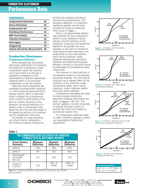
Figure 3CHO-SEAL 1285 and CHO-SIL 1485Sheet Stock Compression-DeflectionCompression-Deflectionspecial shapes.Conductive ElastomersCompression-DeflectionWhile standard test procedures have been established for measuring the deflection of elastomers under compressive loads, the practical use of such data is to provide a qualitative comparison of thedeformability of different elastomeric materials when in the particular configuration of the test sample.Solid (non-foam) elastomers are essentially incompressible materials;i.e., they cannot be squeezed into a smaller volume. When a solid elas-tomer is subject to a compressive load, it yields by deformation of the part as a whole. Because of this behavior, the actual deflection of a gasket under a compressive load depends upon the size and shape of the gasket as well as on its modulus and the magnitude of the load.The design of a seal should be such that it will be subjected to the minimum squeeze sufficient toprovide the required mechanical and electrical performance. The designed deflection of conductive elastomer gaskets should never exceed the maximum deflection limits shown in Table 1.There is an approximate relation-ship between the force required to deflect a pure elastomer a given amount, and the hardness of the elastomer. In general, the harder the elastomer, the greater the force required. In the case of Chomerics’metal particle-filled elastomers, this relationship is much less definite,and in some instances, these materials demonstrate deflection/hardness and deflection/thickness behavior contrary to that which would be anticipated for conventional rubber compounds.The inclusion of metal particles in the elastomer results in a mechanically structured material. This mechanical structure has a marked effect on the deflection of the elastomer under compressive loads, and in some instances, harder materials deflect more than softer materials.Compressive load-deflection data for many popular conductiveelastomer materials and shapes are given in Figures 1-25. (For “linecontact” gaskets, it is more convenient to express the load in terms of pounds per linear inch instead of pounds per square inch).For compression-deflection data on other Chomerics gaskets, contact our Applications Engineering Department.Compression-DeflectionCompression-DeflectionCONTENTS:Compression-Deflection 80Stress Relaxation 83Compression Set 83Shielding Effectiveness 83EMP Survivability 84Vibration Resistance 84Heat Aging 85Outgassing85Volume Resistivity Measurement86Figure 80.125 in. (3.18 mm) Dia. O-Strip Compression-DeflectionDeflection,%Compression-DeflectionCompression-DeflectionL o a d , l b ./i n c hDeflection, %Figure 210.156 in. (3.96 mm) High Hollow D-Strip Compression-DeflectionL o a d , l b ./i n c hDeflection, %Figure 220.312 in. (7.92 mm) High Hollow D-Strip Compression-DeflectionFigure 200.250 in. (6.35 mm) Dia. Hollow O-Strip Compression-DeflectionL o a d , l b ./i n c hDeflection, %L o a d , l b ./i n c hDeflection, %Figure 230.250 in. (6.35 mm) Dia. Hollow P-Strip Compression-DeflectionFigure 240.360 in. (9.14 mm) Dia. Hollow P-Strip Compression-DeflectionL o a d , l b ./i n c hDeflection, %L o a d , l b ./i n c hDeflection,%Figure 190.156 in. (3.96 mm) Dia. Hollow O-Strip Compression-DeflectionL o a d , l b ./i n c hDeflection, %Figure 170.250 in. (6.35 mm) Wide Rectangular Strip Compression-Deflection0.40.81.20.20.61.0C o m p r e s s i o n F o r c e (l b /i n )00.5 1.50.10.2Deflection (inch)1356P/N 10-09-W864-XXXXFigure 250.410 in. (10.41 mm) High V-Strip Compression-DeflectionStress RelaxationAs important as Compression Set and Compression-Deflection, is the Stress Relaxation characteristic of a gasket.If a rubber is subject to a com-pressive load, it will deflect. There is a stress/strain relationship, which for rubbers is generally non-linear except for very small deflections.After the load is applied, a stress decay occurs within the polymer resulting from the internal rearrange-ment of the molecular structure. An approximate rule is that the relaxed stress for cured silicone will finally settle at 70 to 75 percent of the initial stress.There are two ways in which a rubber gasket can be loaded to a desired value. One way is to load it to a point, let it relax, and reapply the load to restore the original stress. The next time it will relax, but not so much.If this is repeated a sufficient number of times, the correct static load on the gasket will reach equilibrium.A more practical way to reach the design value of stress is to load the gasket to 125 percent of its final design value, so that after the relax-ation process is completed the gasket will settle to 100 percent of the design load. This is very reproducible.Figure 26shows a typical stress relaxation curve for Chomerics’conductive elastomers.Compression SetWhen any rubber is deformedfor a period of time, some of the defor-mation is retained permanently even after the load is removed. The amount of permanent deformation, asmeasured by ASTM D395, is termed “Compression Set.” Compression set is measured under conditions of constant deflection (ASTM D395Method B) and is normally expressed as a percentage of the initialdeflection, not as a percentage of the initial height.For gaskets that are used once, or where the gasket/flange periphery relationship is constant (such as a door gasket), compression set is of minor significance if the original load condition and the service temperature are within the design limitations of the gasket material.For gaskets that are randomlyreseated one or more times in normal service life, it is important that the maximum change in gasket thickness does not exceed twice the maximum mismatch between the opposing mating surfaces.Shielding EffectivenessMost shielding effectiveness data given in Table 3 of the Conductive Elastomer section (pages 32-34) is based on a MIL-G-83528B testmethod, with a 24 in. x 24 in. aperture in a rigid enclosure wall and about 100 psi on the gasket. It is a valid and useful way of comparing variousgasket materials, but does not reflect the shielding effectiveness one can expect at seams of typical enclosures.CHO-TM-TP08 is a modified version of the MIL test that provides typical values achieved in actual applications.Since many factors will affect the actual shielding effectiveness of anenclosure seam (flange design,stiffness, flatness, surface resistivity,fastener spacing, enclosuredimensions, closure force, etc.), the only way to determine shielding effectiveness for real enclosures is to test them.Figures 28and 29provide dataon shielding effectiveness for actualFigure 27Formula for Calculation of Compression Setenclosures. The data in Figure 28shows the difference in attenuation between a shelter door closed with no gasket and the same door closed against a CHO-SEAL 1215 hollow D-strip gasket. Instead of single data points at each frequency tested, a range of data is shown for eachfrequency, representing the worst and best readings measured at many points around the door. Figure 29 shows the effects of closure force on shielding effectiveness of an enclosure tested at high frequencies (1-40 GHz) using CHO-SEAL 1215 solid D-strip gaskets.In order to establish reasonable upper limits on gasket resistivity, it is necessary to understand the rela-tionship between flange interface resistance and EMI leakage through the flange. Figure 30presents this relationship for an aluminum enclosure 3 in. x 3 in. x 4 in. deep, measured at 700 MHz. Die-cut gaskets 0.144 in.wide by 0.062 in. thick, in a wide range of resistivities, were clamped between the gold-plated flanges of thisenclosure. Simultaneous measure-ments of flange interface resistance (all attributable to the gaskets) versus RF leakage through the seamproduced a classic S-shaped curve.For the gasket configuration used in this test, the dramatic change in shielding effectiveness occursbetween gasket volume resistivities of 0.01 and 0.4 ohm-cm. Since real enclosures do not have gold-plated flanges, but rather have surfacefinishes (such as MIL-C-5541 Class 3chromate conversion coatings) which also increase in resistance over time, it is recommended that gasket volume resistivity be specified at 0.01 ohm-cm max. for the life of the equipment.Frequency, HzA t t e n u a t i o n (dB )Figure 28Shielding Effectiveness of a Shelter Door Gasket (14 kHz to 10 GHz)kA/inch of gasket (peak-to-peak).Pure silver (1224) and silver-plated-aluminum filled (1285) gaskets have less current carrying capability than silver-plated-copper materials, but are generally acceptable for EMP hardened systems (depending on specific EMP threat levels, gasket cross section dimensions, etc.).Vibration ResistanceCertain conductive elastomers are electrically stable during aircraft-level vibration environments, while others are not. The key factor which deter-mines vibration resistance is theshape and surface texture of the filler particles. Smooth, spherical fillers (such as those used in silver-plated-Figure 32Scanning Electron Microscopy Illustrates EMP Damage Mechanism for Silver/Glass ElastomersL e a k a g e (d B )Vibration (g)Figure 33Effects of Vibration on Shielding Effectiveness of Conductive Elastomer GasketsEMP SurvivabilityIn order for an enclosure to continue providing EMI isolationduring and after an EMP environment,the conductive gaskets at joints and seams must be capable of carrying EMP-induced current pulses without losing their conductivity. Figure 31shows the EMP current response of various types of conductive elastomer gaskets. Note that gaskets based on silver-plated-glass fillers (1350)become nonconductive at low levels of EMP current, and should therefore not be used when EMP is a design consideration. Figure 32is an electron microscope photo which clearly shows the damage mechanism.Silver-plated-copper filled (1215)gaskets have the highest resistance to EMP type currents, showing no loss of conductivity even at 2.50102030405060Shielding Degradation, dBIn t e r f a c e R e s i s t a n c e , m i l l i o h m sFigure 30Interface Resistance vs. Shielding Degradation at a Flange Jointglass materials) tend to move apart during vibration, leading to dramatic increases in resistance and loss of shielding effectiveness (although they normally recover their initial properties after the vibration has ended). Rough, less spherical particles resist vibration with very little electrical degradation. Figure 33shows the effects of vibration on three types of conductive gaskets.Although Chomerics’ silver-plated-copper filled 1215 gasket, with rough,irregular particle agglomerations,exhibits excellent stability during vibration, users of conductive elastomers should be aware that smooth, spherical silver-plated-copper fillers can be almost asunstable as silver-plated-glass fillers.Frequency, GHzA t t e n u a t i o n (dB )Figure 29Effect of Closure Force on Shielding Effectiveness (1 GHz to 40 GHz)Heat AgingThe primary aging mechanism which affects electrical stability of conductive elastomers is the oxidation of filler particles. Formaterials based on pure silver fillers,particle oxidation is not generally a problem because the oxide of silver is relatively soft and reasonably conductive. If the filler particles are non-noble (such as copper, nickel,aluminum, etc.) they will oxidize readily over time and become nonconductive. Even silver-plated base metal powders, such as silver-V o l u m e R e s i s t i v i t y (o h m -c m )Hours at 150°C (Solid Line)Hours at 125°C (Dotted Line)Figure 34Typical heat aging characteristics of Chomerics’ plated-powder-filled conductiveelastomers. Flanged 1000-hr test recommended for qualification. Unflanged 48-hr. test recommended for QC acceptance.plated-copper or silver-plated-aluminum will become non-conductive over time if the plating is not done properly (or if other processingvariables are not properly controlled).These are generally batch control problems, with each batch being potentially good or bad.The most reliable method of predicting whether a batch will be electrically stable is to promote the rate at which poorly plated or processed particles will oxidize, by heat aging in an air circulating oven.For qualification, 1000 hours (42 days)at maximum rated use temperature (with the gasket sample deflected 7-10% between flanges) is the recommended heat aging test for accelerating the effects of long-term aging at normal ambient tempera-tures. A quicker heat aging test,which correlates well with the 1000hour test and is useful for QC acceptance testing, involves a 48hour/150°C oven bake with thegasket sample on an open wire-grid tray (rather than being clamped between flanges). Figure 34shows typical data for volume resistivity versus time for each of these tests.Note:It is essential that no source of free sulfur be placed in the aging oven, as it will cause the material to degrade electrically and mask any oxidation aging tendencies. Common sources of sulfur are neoprenes,most cardboards and other paper products.OutgassingMany spacecraft specifications require that nonmetallic components be virtually free of volatile residues which might outgas in the hard vacuum environment of space. The standard test method for determining outgassing behavior is ASTM E595-93, which provides for measurement of total mass loss (TML) and collected volatile condensable materials (CVCM) in a vacuum environment. Data for a number of Chomerics conductive elastomers,based on ASTM E595-93 testing done by NASA Goddard SpaceflightCenter, is presented in Table 2. The normal specification limits or guide-lines on outgassing for NASA applications are 1% TML max.,and 0.1% CVCM max.。
user manual for reflow head NA-66

If the user igflores this warning and mishandles the
WAR NI N G
product, death to the it may user. result 『serious and fatal ipiuhe user ignores this caution and mishandles the product, it may result in i'ury to the user, or material damages.
(2) Aftercare Service
When you have a trouble on the system, check the unit for the trouble with reference to this manual. If the trouble cannot be fixed with any attempts, please make a contact to 小e maintenance service center shown below.
(助 Repair after the period of guarantee
If the system can be maintained its function 饰 repair work, we will acce眯 repair request Minimum time of guarantee for stock of key parts is 7 years after the termination of manufacturing.
(3) Repair during the Guarantee Period
Reflow profile 解读

怎样设定锡膏回流温度曲线
接下来必须决定各个区的温度设定,重要的 是要了解实际的区间温度不一定就是该区的显 示温度。显示温度只是代表区内热敏电偶的温 度,如果热电偶越靠近加热源,显示的温度将 相对比区间温度较高,热电偶越靠近PCB的直 接通道,显示的温度将越能反应区间温度。
怎样设定锡膏回流温度线
典型PCB回流区间温度设定 区间 预热
RTS温度曲线可用于任何化学成分或合金,为水溶锡膏和难 于焊接的合金与零件所首选。 RTS温度曲线比RSS有几个优 点。RTS一般得到更光亮的焊点,可焊性问题很少,因为在 RTS温度曲线下回流的锡膏在预热阶段保持住其助焊剂载体 。这也将更好地提高湿润性,因此,RTS应该用于难于湿润 的合金和零件。
得益于升温-到-回流的回流温度曲线
得益于升温-到-回流的回流温度曲线
升温-保温-回流 RSS温度曲线开始以一个陡坡温升,在90秒的目标 时间内大约150° C,最大速率可达2~3° C。随 后,在150~170° C之间,将装配板保温90秒钟; 装配板在保温区结束时应该达到温度均衡。保温 区之后,装配板进入回流区,在183° C以上回 流时间为60(± 15)秒钟。
理解锡膏的回流过程
2.
3.
助焊剂活跃,化学清洗行动开始, 水溶性助焊剂和免洗型助焊剂都会 发生同样的清洗行动,只不过温度 稍微不同。将金属氧化物和某些污 染从即将结合的金属和焊锡颗粒上 清除。好的冶金学上的锡焊点要求 “清洁”的表面。 当温度继续上升,焊锡颗粒首先单 独熔化,并开始液化和表面吸锡的 “灯草”过程。这样在所有可能的 表面上覆盖,并开始形成锡焊点。
升温-到-回流
因为RTS曲线的升温速率是如此受控的,所以 很少机会造成焊接缺陷或温度冲击。另外, RTS曲线更经济,因为减少了炉前半部分的加 热能量。此外,排除RTS的故障相对比较简单, 有排除RSS曲线故障经验的操作员应该没有困 难来调节RTS曲线,以达到优化的温度曲线效 果。
Harvard_Referencing(英文要点讲解)

• Many departments at universities believe it is unethical to plagiarize. Therefore, referencing is essential to avoid what is perceived as unethical behaviour.
2. Initial of
first name
6. Editor(s) name(s) ed=editor eds=editors
7. Publisher
8. Place (city)
of publication
9. Page Range
IFf othreEaxuatmhoprleh:as a middle name on the
• You will be able to produce a reference list entry for an article from an edited book and a Webpage
• You will be able to use in-text citation to reference an article from an edited book and a Webpage
6. Cut and paste the URL Put it between <arrow brackets> Remove the hyperlink
3.Article title
4.URL
纹理物体缺陷的视觉检测算法研究--优秀毕业论文
摘 要
在竞争激烈的工业自动化生产过程中,机器视觉对产品质量的把关起着举足 轻重的作用,机器视觉在缺陷检测技术方面的应用也逐渐普遍起来。与常规的检 测技术相比,自动化的视觉检测系统更加经济、快捷、高效与 安全。纹理物体在 工业生产中广泛存在,像用于半导体装配和封装底板和发光二极管,现代 化电子 系统中的印制电路板,以及纺织行业中的布匹和织物等都可认为是含有纹理特征 的物体。本论文主要致力于纹理物体的缺陷检测技术研究,为纹理物体的自动化 检测提供高效而可靠的检测算法。 纹理是描述图像内容的重要特征,纹理分析也已经被成功的应用与纹理分割 和纹理分类当中。本研究提出了一种基于纹理分析技术和参考比较方式的缺陷检 测算法。这种算法能容忍物体变形引起的图像配准误差,对纹理的影响也具有鲁 棒性。本算法旨在为检测出的缺陷区域提供丰富而重要的物理意义,如缺陷区域 的大小、形状、亮度对比度及空间分布等。同时,在参考图像可行的情况下,本 算法可用于同质纹理物体和非同质纹理物体的检测,对非纹理物体 的检测也可取 得不错的效果。 在整个检测过程中,我们采用了可调控金字塔的纹理分析和重构技术。与传 统的小波纹理分析技术不同,我们在小波域中加入处理物体变形和纹理影响的容 忍度控制算法,来实现容忍物体变形和对纹理影响鲁棒的目的。最后可调控金字 塔的重构保证了缺陷区域物理意义恢复的准确性。实验阶段,我们检测了一系列 具有实际应用价值的图像。实验结果表明 本文提出的纹理物体缺陷检测算法具有 高效性和易于实现性。 关键字: 缺陷检测;纹理;物体变形;可调控金字塔;重构
Keywords: defect detection, texture, object distortion, steerable pyramid, reconstruction
II
Accuri_CFlow_Software_Guide

CFlow User Guide Science is hard. Flow cytometry should be easy.®Table of ContentsChapter 1 The Basics - Operating the Accuri® C6 Flow Cytometer® (4)Introduction to CFlow and Running the C6 (4)CFlow Workspace (4)Getting Started (4)Running Validation Beads (6)Saving the Data (7)Analyzing and Recording your Validation Bead Data (8)Troubleshooting (12)Chapter 2 Getting the Most from the C6 (13)Materials Needed to Operate and Maintain the C6 (13)System Cleaning and Validation (13)Standard Operating Procedures for the C6 (14)Routine Instrument Maintenance (15)Tips on Data Collection and Analysis with the C6 (16)Chapter 3 Using the Collect Tab (17)Introduction (17)Experimental Design of Tutorial File (17)Opening a New CFlow Workspace and Collecting a Data File (18)Creating Plots and Applying Gates (20)Adding Data to a CFlow File and Naming Plot Axes (24)Naming and Saving a CFlow File (26)Calculating Median Values and Applying Fluorescence Compensation (27)Adding and Applying Additional Gates (32)Adjusting the Axes View Using the Plot Spec Tool (Zooming) (34)Chapter 4 Using the Analyze Tab (36)Make an Overlay Histogram in Analyze Tab (41)Chapter 5 CFlow Software Menus (42)The File Menu (42)The Edit Menu (43)The About Menu (48)Chapter 6 VirtualGain (49)Applying VirtualGain (50)Chapter 7 CFlow Sampler (56)Introduction (56)The Manual Collect Tab (58)Using the Manual Collect Tab (60)The Auto Collect Tab (61)Creating Sample Sets and Applying Acquisition Settings (62)The Run Display (65)Analyze and Statistics Tabs (67)Running a Sample Plate (Example) (68)Collisions and Alignment (69)Table of FiguresFigure 1-1 The CFlow Control Panel in detail (5)Figure 1-2 C6 Improper Shut Down Recovery Message (6)Figure 1-3 Saving a CFlow file (8)Figure 1-4 Proper position of R1 on Plot 1 and Gate selection for Plot 2 (9)Figure 1-5 Location of Zoom Tool and Expand Tool, and effect of Zoom (9)Figure 1-6 Example of 8-peak bead data collected with a C6. The number of expected peaks is: FL1-H (8), FL2-H (8) and FL3-H (6). The peaks in FL4-H are not relevant. (10)Figure 1-7 Example of 6-peak SPHERO APC Calibration Particles, shown in FL4-H. The peaks in FL1-H, FL2-H and FL3-H are not relevant. (11)Figure 1-8 Statistics tab Display of 8-peak bead data from successive days (12)Figure 2-1 Zoom tool used to focus on lymphocyte light scatter and surface marker fluorescence (16)Figure 3-1 CFlow Workspace after selecting File, New CFlow File from the CFlow file menu (18)Figure 3-2 The Plot Spec Dialog Box. Changing these settings only affects the view of the data. No data is changed in, or lost from, the data file. (18)Figure 3-3 Threshold Settings dialog box (19)Figure 3-4 Warning message when raising a threshold value will result in data loss (19)Figure 3-5 CFlow template after collection of Sample A1, human peripheral blood (20)Figure 3-6 Use of Zoom Tool for a “close-up” view of the lymphocyte population in a human peripheral blood sample. (20)Figure 3-7 Polygonal gating tool was used to draw P1 on the 2D plot above. Other available gating tools are Rectilinear and Quadrant. (21)Figure 3-8 Opening a Density plot defaults to a linear FSC-A vs. SSC-A plot. (21)Figure 3-9 Changing density plot axes parameters and scaling (22)Figure 3-10 Selecting a gating option, which includes all events from a given gate, i.e. Plot 2 is now gated to Include “P1 on all events” (22)Figure 3-11 Plot 2 has been gated to include P1 (all events). (23)Figure 3-12 Gating choice options for plots: Include, Exclude, and Intersection. (23)Figure 3-13 Adding Vertical or Quadrant Markers to the Gating list. (23)Figure 3-14 Selecting to display the 1st decade of data on a default log data plot. a. Open the Plot Spec dialog box. b. Uncheck “Hide 1st decade” boxes for FL1-A and FL2-A, and set the “Min Value” for both parameters to 0. (24)Figure 3-15 A CFlow Workspace with 5 added 2D fluorescence plots. Plots required for tutorial: FL1-A vs. FL2-A; FL1-A vs. FL3-A; FL2-A vs. FL3-A; FL4-A vs. FL3-A; FL1-A vs. FL4-A. (24)Figure 3-16 Sample number 2 has been added to well A2 in the CFlow Workspace. (25)Figure 3-17 Changing axes labels using the axis label drop-down menu and the Rename Parameters option. (25)Figure 3-18 Changing axes labels using the axis label drop-down menu and the Rename Parameters option. Note that once the label CD45 PE-Cy7 has been entered it will now appear in the drop-down menu when the Select option is chosen. (26)Figure 3-19 Saving and naming a CFlow File. (26)Figure 3-20 New file name, “Human PB”, appears in the upper left corner of the CFlow workspace after saving and naming the CFlow file. (27)Figure 3-21 Fluorescence spillover of positive PE-Cy7 signal from FL3 into a. FL1-A, and b. FL2-A, c. The PE-Cy7 signal does not spillover into FL4-A. (27)Figure 3-22 Selection and placement of Quadrant Marker (27)Figure 3-23 a. Placement of Quadrant Tool for Median calculations on the double negative (lower left) and single PE-Cy7 positive (upper left) populations. b. Median fluorescence values in the Statistics Table for Plot 3, Q1, will all read “NA” until Calculate Median is selected. (28)Figure 3-24 Quadrant Q2 is selected with mouse click (indicated by bold red) and Calculate Median chosen from the Display drop-down menu. (28)Figure 3-25 Statistics Table updated with median values after choosing Calculate Median from the Display drop-down menu. (29)Figure 3-26 Opening and using the Compensation Settings dialog box. (29)Figure 3-27 Results of subtracting spillover of FL3 PE-Cy7 signal from FL1 by 1.35%. Note that the median FL1 channel numbers in Q1-UL (238) and Q1-LL (231) are approximately equal (blue boxes). .. 29 Figure 3-28 Results of selecting Plot 4, applying Quadrant markers and calculating Median fluorescence channel values. (30)Figure 3-29 Results of correcting FL2 by subtracting 4.3% of the signal from FL3 (PE-Cy7). The Median FL2 fluorescence channel value for Q2-UL (131) is approximately equal to the Median FL2 fluorescence channel value for Q2-LL (134). (31)Figure 3-30 No fluorescence subtraction of FL3 PE-Cy7 signal is needed from FL4, as indicated by comparison of Median FL4 values for Q3-UL (290) and Q3-LL (263). (31)Figure 3-31 Correction of spillover from FITC FL1 into FL2. a. Before fluorescence subtraction. b. After calculation and application of appropriate percentage subtraction of FL1 from FL2. (32)Figure 3-32 Gating region R1 has been drawn on Plot 3 to include the CD45-PE-Cy7 positive events. (32)Figure 3-33 Gating Plot 2 (CD3-FITC vs. FL2-A) to include events in gates R1 and P1 (33)Figure 3-34 Gate for Plot 2 (CD3-FITC vs. FL2-A) includes events in gates R1 and P1, after following steps 1-3 in Adding and Applying Additional Gates. (34)Figure 3-35 Blue boxes show desired 4 log channel to view for Plots 2 and 6. (34)Figure 3-36 Setting Min and Max channel values for the X and Y axes using the Plot Spec dialog box. .. 35 Figure 3-37 Result of axes view adjustment to 4 logs for Plots 2 and 6. (35)Figure 4-1 The Analyze Tab (36)Figure 4-2 Selecting plots to copy from the Collect tab. (37)Figure 4-3 Plots 1C, 3C and 6C opened in the top row of Analyze tab (37)Figure 4-4 Analyze tab with copied plots in Plot List and selected plot corral. (38)Figure 4-5 Analyze Tab: Result of gating Plot 3C on "P2 in all" and Plot 6C on "R2 in (P2 in all)" (38)Figure 4-6 Analyze Tab: Row 2 selected to display data from Sample A2 in Plots 1C, 3C and 6C. (39)Figure 4-7 Analyze Tab view after scrolling down to empty plot corrals. (39)Figure 4-8 Analyze Tab view after adding 2 more rows of Plots 1C, 3C and 6C, and populating with data from Sample A3 and A4. (40)Figure 4-9 Analyze Tab: Plots are selected for printing. (40)Figure 4-10 Analyze tab: Overlay Tool has been selected. (41)Figure 4-11 Analyze tab: Overlays of FL1-A data for samples A2, A3 and A4. The Overlay Legend has been opened. (41)Figure 5-1 The File Menu (42)Figure 5-2 The Edit Menu (43)Figure 5-3 Rename Parameters (43)Figure 5-4 Rename Parameters, selection options menu (44)Figure 5-5 The Display Menu (44)Figure 5-6 Events Display Settings (44)Figure 5-7 a. Quadrant marker is not selected b. Quadrant Marker selected (bold lines) (45)Figure 5-8 a. Statistics table before selecting Calculate Median b. Statistics table after selecting Calculate Median (45)Figure 5-9 a. Statistics table after moving Quadrant markers (45)Figure 5-10 The Instrument Menu (46)Figure 5-11 Threshold Settings (46)Figure 5-12 Warning displayed after a change in threshold settings (47)Figure 5-13 Compensations Settings (47)Figure 5-14 The About Menu (48)Figure 6-1 When to use VirtualGain (49)Figure 6-2 Recreate the histogram or copy plots from Collect (50)Figure 6-3 Click on the histogram parameter label to reveal the Parameter list. (50)Figure 6-4 Step 7 and Step 8, Aligning plots. (51)Figure 6-5 Step 9, Pick the sample to align. (52)Figure 6-6 Step 11, Move the Peak Definition Marker. (52)Figure 6-7 Step 14, To align other samples exactly as the first aligned sample. (53)Figure 6-8 Step 15, A black asterisk appears under the Sample to Align plot. (53)Figure 6-9 The sample with VirtualGain applied has a black asterisk under the parameter label. (54)Figure 6-10 Click the asterisk to switch between VirtualGain and native displays. A grey asterisk indicated native data, a black one Virtual Gain applied (54)Figure 6-11 Overlays automatically display VirtualGain whenever applied. (55)Figure 7-2 The Plate Type drop-down menu. (57)Figure 7-1 CFlowSampler start-up screen. (57)Figure 7-3 The CFlowSampler Manual Collect Tab. (58)Figure 7-4 The Run Backflush Cycle window. (59)Figure 7-5 The Run Unclog Cycle window (59)Figure 7-6 The Calibrate Fluidics window. (60)Figure 7-7 The Auto Collect tab (61)Figure 7-8 Selecting an individual sample. (62)Figure 7-9 Applying settings to a set of samples will turn those sample wells the same color. (63)Figure 7-10 The Auto Collect tab displaying two sets. (63)Figure 7-11 The Run Display (65)Figure 7-12 The Run Display while collecting data. (66)Figure 7-13 The CSampler display after completion of a sample run. (67)Figure 7-14 Collision detected window (69)Chapter 1 The Basics - Operating the Accuri® C6 Flow Cytometer®Introduction to CFlow and Running the C6The C6 Flow Cytometer system includes CFlow or CFlow Plus software for controlling the instrument, acquiring data, generating statistics, and analyzing results. Throughout this User Guide, CFlow refers to both CFlow and CFlow Plus unless indicated otherwise.CFlow WorkspaceThe CFlow workspace provides access to all the functions needed to acquire and analyze data. CFlow is divided into three separate tabs: Collect,Analyze and Statistics. This section focuses on data acquisition and the Collect tab.The Collect tab appears when CFlow is launched and is used to acquire data from samples processed on the C6. The Collect tab enables physical control of the C6, provides access to settings needed to specify the threshold and stop criteria as well as many analytic functions.Figure 1-1 shows a partial Collect tab. The Sample Grid is laid out in the configuration of a 96-well plate to facilitate both organization of experiments and data acquisition from sample tubes. CFlow acquires each sample into its own well in the Sample Grid. The wells can be filled with data in any order that is convenient. White wells do not contain data and are available to use for data collection. Blue wells contain data. A red outline around a well indicates that well is currently selected for viewing or collecting data.Instrument ControlsThe left-hand column of the CFlow Collect tab provides access to all instrument controls needed to collect data. Before data collection can begin, the Traffic Light below the Sample grid must be green and the words “C6 Cytometer is connected and ready” appear in the message box.Getting StartedThis section provides a step-by-step guide for running validation beads. The validation will demonstrate many of CFlow features and ensure the C6 is working properly before running experimental samples. All the individual features of CFlow are described in detail in Chapter 4.Complete the initial instrument set-up as outlined in the C6 Flow Cytometer Instrument Manual, Section 4, before continuing.Starting CFlowOpen CFlow by double clicking on the CFlow icon on the desktop. The message box in CFlow will say Cytometer Not Connected.C6 Startup Procedure1. Check sheath bottle (blue ring) fluid level and fill if needed. Accuri recommends the use of 0.2 µmfiltered, deionized, H2O with bacteriostat added (Accuri Part# KR-220). CFlow will alert the user if the bottles need attention when the C6 is turned on and CFlow is running.2. Empty the waste tank (red ring).3. Check Cleaner (green ring) and Decontamination Solution (yellow ring) bottles. Fill if necessary.Refer to C6 Flow Cytometer Instrument Manual, Section 4.3.Figure 1-1 The CFlow Control Panel in detail4. Replace the tube on Sample Introduction Probe (SIP) with a fresh tube containing at least 2 mLfiltered, deionized H 2O.5. Firmly press the On/Off button on the front of the unit to turn on the C6. A blue light will flash and thenstay illuminated. After ~20 seconds, the CFlow traffic light will show yellow. After ~60 seconds, the C6pumps will start to run. When powered on, the C6 will automatically flush the fluidics lines with sheath. This process takes approximately 3 minutes. 6. When the C6 is ready for data collection, the CFlow traffic light will change to green. Begin data Sample Naming Field Set Threshold : Default is 80,000 on FSC-HRun: Click to Start Sample Acquisition Reads PAUSE during acquisition;reads ADD TO when the well is doneand/or already contains data.Opens Color Compensation Matrix Real-TimeAcquisition/Counter DisplayStatus Bar Traffic Lightand Message BoxBackflush and UnclogControls Delete: Permanently Deletes allEvents from Sample Fluidics Control :Sample Rate Adjustment96-Well Sample GridCustom Fluidics Settings:User-Defined Flow Rate andCore Size, User-DefinedStop Criteria (CFlow Plusonly) Custom Fluidics Settings: User-Defined Flow Rate andCore Size, User-Defined StopCriteria (CFlow Plus only)collection when the Traffic Light is green and the C6 Status Message Box reads C6 and CFlow are connected and ready.For optimal performance, the C6 should be on for at least 15 minutes prior to processing samples.C6 Improper Shut Down Recovery MessageIf the message shown in Figure 1-2 is seen at startup, the C6 will take approximately 6 minutes to recover and return to the green-light, ready state, as opposed to the usual 3 minute startup procedure. This may occur on initial C6 startup when the unit is first received. It will also occur after an interruption of power to the unit.Figure 1-2 C6 Improper Shut Down Recovery MessageRunning Validation BeadsAccuri provides an initial set of pre-diluted validation beads. Store the beads at 4°C in the dark. The beads expire within 2 weeks of receipt. Refer to Reagents Required for ordering information.Validate the performance of the C6 with validation beads each day that the cytometer is used. The C6 should be able to distinguish a defined number of peaks within each fluorescence channel. If these peaks are not discernable there may be a problem and any data collected may be flawed.It is important to collect and save a bead data file every day that data is collected. The user can easily address many C6 issues with assistance from Accuri Technical Support. If a problem is experienced that requires telephone assistance, Technical Support may ask for data from the bead file to assist in troubleshooting.Reagents Required1. Spherotech 8-Peak Validation Beads (Accuri Part# QA-100) or the prediluted 12x75 mm tube fromAccuri labeled 8-Peak Beads2. Spherotech 6-Peak Validation Beads (Accuri Part# QA-110) or the prediluted 12x75 mm tube fromAccuri labeled 6-Peak Beads3. Sheath fluid: Deionized, filtered water (0.2 µm filter) plus Bacteriostatic Concentration Solution (AccuriPart# KR-220)Running the Bead Samples1. Be sure that the C6 has been switched on for at least 15 minutes.2. Verify that the file named “Bead Template.c6t” has been copied to the computer attached to the C6.This file is on the CFlow CD shipped with the C6 and also available on the Accuri website.3. Double-click on the bead template file to open or load the file from the CFlow File Menu.4. Place an empty 12x75 mm tube on the SIP.5. Click on “BACKFLUSH”.6. Place a fresh tube with 2 mL filtered, deionized H2O on the SIP.7. Click on well A1 to select it. Well A1 should now have a red box around it.8. Deselect the Run Unlimited check box under Run Limits in the Instrument Control Panel.9. Select the time check box (Min Sec) in the Instrument Control Panel and input 2 minutes.10. In the Control Fluidics section of the Control Panel, select Slow. The flow rate should display14µL/min and Core Size should display 10 µm.11. Click on the Threshold button to set the Threshold to 80,000 on FSC-H (default).12. Press Run. While data is being acquired, well A1 will flash blue.13. Click Pause then the Delete Sample Data button in the Control Panel of the CFlow screen to cleardata collected during the run. The data well should change from blue to white and the counters will reset.14. Deselect the time check box and click the Events check box. Verify that it is set to 50,000 events inUngated Sample. If not, enter 50,000 events and select the Ungated Sample check box.15. Replace the tube on the SIP with a tube containing suspended 8-peak beads. Vortex the tube prior toplacing it on the C6.16. Click RUN to start acquisition. Acquisition will automatically stop after 50,000 total events areacquired. Do not click on ADD TO. ADD TO is used to add more data to a well that already contains data. The R1 region may not encompass the main population of bead events on the FSC-H vs. SSC-H plot. This will be addressed in Analyzing and Recording Your Validation Bead Data.17. Name this sample including the date processed in the text box just above the Sample Grid. Samplescan be named at any time; before, during, or after collection.18. Remove the beads tube and wipe off the end of the SIP with a Kimwipe, or comparable material, tominimize bead carryover. To further minimize carryover, click Backflush while holding a reservoir or empty tube under the SIP. Fluid should drip or stream out of the SIP.19. Place a tube with suspended 6-peak beads on the SIP. Vortex the tube prior to use.20. Click on well E1 to advance to well E1. Verify that the Events check box is still selected and set to50,000 events in Ungated Sample.21. Click RUN. The R2 region on the FSC-H vs. SSC-H plot in the second row of the CFlow bead file maynot encompass the main population of beads.22. Name this sample including the current date in the text box just above the Sample Grid.23. Remove the beads tube from the SIP and wipe the end of the SIP.24. Place a tube with 2 mL of filtered, deionized H2O on the SIP and advance to any empty data well.25. Select the time check box (Min Sec) in the Instrument Control Panel and set it for 2 minutes. ClickRUN.26. Leave the tube on the SIP after the C6 stops running.Always end each data collection session on the C6 by running filtered, deionized H2O for 2 minutes. Leave this tube on the SIP between sessions and when shutting off the C6.Saving the DataSaving data as a CFlow file will save the CFlow workspace in its entirety, including collected sample data, plot layouts, gating, color compensation, and threshold settings that have been added. Changes made in the Collect, Analysis or Statistics tabs will be saved in a single comprehensive (and often large) data file. Data collected on the C6 should always be saved as a CFlow file.There is no need to export after every sample run. Data from individual sample wells can be exported from CFlow as FCS 3.0 files at any time.Save Your Data as a CFlow File1. In CFlow, under the File menu select Save CFlow File (Figure 1-3) and save the bead data file as a“Validation Bead File”. Use this file each day to collect Validation Bead data, advancing to a new well in row A or E for 8-peak and 6-peak beads, respectively. Include the date in the Sample Naming Field when naming each day’s bead sample.CAUTION: CFlow does not automatically save CFlow files to the computer hard drive. The data is saved locally in RAM until it is saved as a CFlow file or exported as FCS files. CFlow allows switching between data wells to view data even when data is not stored to the hard drive.2. End every session of data collection on the C6 by placing a tube containing 2 mL of filtered, deionizedH2O on the SIP. Run for 2 minutes in an empty data well to clear the last sample’s residue from the SIP. Leave the tube on the SIP after the run has finished.Figure 1-3 Saving a CFlow fileAnalyzing and Recording your Validation Bead DataAnalyze the bead data using the Collect tab of CFlow.1. Click on the well in the Bead File which contains the 8-peak bead data to select it (will be A1 iffollowing previous procedure).2. On the first FSC-H vs. SSC-H plot (scatter plot) in the bead file, adjust the pre-drawn region R1 toencompass the main population by clicking on the region (it will have thicker lines when selected) and dragging it so it looks like Plot 1 in Figure 1-4. This should contain 75-85% of all events in R1. There is usually a “shadow” population slightly higher in FSC-H than the main cluster of beads; this is normal for these particular beads (bead doublets or clumps). Do not include this group in R1.3. View the next 3 plots - FL1-H, FL2-H, and FL3-H. They should be gated on the scatter region, R1.The phrase “R1 in all” should be visible next to the gray “GATE” button at the top of each of these 3 fluorescence plots (Figure 1-5). If not, click the GATE button and select the option “R1 on all events”from the pop-up gating list.4. Position the predrawn horizontal Marker Region around the top (brightest, far-right) peak on each ofthe 3 fluorescence plots.Use the Zoom Tool, located in the lower right corner of each plot (the button with the magnifying glass),to zoom in on the top peak. Then, adjust the marker tightly around the peak. Click on the Expand Tool (the button with a square and four arrows) to zoom back out.5. Compare the bead run to the manufacturing results sent with the C6. If the C6 is performing properly,data should look similar to that in Figure 1-6 for the 8-peak beads. There should be one mainpopulation of beads on FSC-H vs. SSC-H, 8 discernable peaks on FL1-H and FL2-H, and 6 peaks onFL3-H. FL4-H performance will be checked with the 6-peak beads in a later step.Figure 1-4 Proper position of R1 on Plot 1 and Gate selection for Plot 2A. Before ZoomB. AfterZoom Figure 1-5Location of Zoom Tool and Expand Tool, and effect of Zoom Expand ToolZoom ToolGateAppliedFigure 1-6 Example of 8-peak bead data collected with a C6. The number of expected peaks is: FL1-H (8), FL2-H (8) and FL3-H (6). The peaks in FL4-H are not relevant.6. Select the well containing the 6-peak bead data (should be well E1).7. Adjust the pre-drawn region R2 in the second FSC-H vs. SSC-H to encompass the main data peaksimilar to the procedure for the 8-peak beads. This population should look like an exclamation mark.The R2 region should encompass both major populations (Figure 1-7).8. Confirm that the FL4-H plot is gated on the region R2. If not, click on the “GATE” button and selectthe option “R2 on all events” from the pop-up menu.9. Adjust the Marker in the FL4-H plot to be tightly placed around the top (brightest) peak. Refer toFigure 1-7 for an example of good 6-peak bead data on a C6.10. Record the number of peaks, the Mean channel numbers and CVs for the top peaks, and for theforward scatter of the beads for each parameter in the Accuri Cytometer Log. Additional copies can be found on the CFlow CD and on the Accuri website.Please send a copy of the bead file, from the first time beads are run on the C6 after installation, toAccuri Technical Support: dmack@.Figure 1-7 Example of 6-peak SPHERO APC Calibration Particles, shown in FL4-H. The peaks in FL1-H, FL2-H and FL3-H are notrelevant.Using the Statistics Tab in CFlow to Generate a Table of Mean Peak Channel andCV valuesA convenient way to monitor the Validation Bead data, and thus the C6 performance, is to store the 8-and 6- peak validation bead data in a single CFlow file, saving the data from each day in its own well.Then, using the Statistics tab, a table can be created of the Mean channel numbers and CVs for the toppeaks, and for the forward scatter of the beads to make it easy to determine if the C6 performance isstable.In Figure 1-8, the C6 in question had been performing with a FSC-H CV of between 2% and 2.5% for overa month using the SPHERO Rainbow Calibration Particles. However, on the last day shown, the FSC-HCV had increased substantially as had the top peak CVs for FL1-H and FL2-H. This could indicate eitherbead degradation or a slightly dirty flow cell. Refer to Troubleshooting for possible fixes.Also refer to Troubleshooting if any of the following conditions are experienced:1. Very broad or multiple peaks for FSC-H on the 8- or 6-peak beads, excluding the shadow doubletpopulation, or2. Fewer than 8 peaks visible on FL1-H and/or FL2-H, or fewer than 6 peaks on FL3-H, or3. Brightest peak CVs are >5.0% in any channel.FSC-H CV hasincreased from 2% to3.9%Figure 1-8 Statistics tab Display of 8-peak bead data from successive daysTroubleshootingIf there are very broad or multiple peaks for FSC-H, fewer than 8 peaks visible on FL1-H and/or FL2-H, fewer than 6 peaks on FL3-H or the brightest peak CVs are >5.0% in any channel check the following: 1. If bead data was acquired using the Slow rate (Under Fluidics Control in the Control Panel). If not,select Slow, re-suspend the beads by vortexing or flicking the tube, and recollect the data.2. The age of the beads. If the beads have been diluted for more than 2 weeks, kept at roomtemperature or warmer, or exposed to light for long periods of time, their performance may be degraded. Make up new bead suspensions and run the bead sample again.3. If there is a bubble or clog in the flow cell.a. Run the bead sample again.b. Remove the tube from the SIP, place an empty tube under the SIP and click Unclog. Whenthe Unclog cycle is finished (Traffic Light will be green), run the bead sample again.c. Remove the tube from the SIP, place an empty tube under the SIP and click Backflush.When the cycle is finished (Traffic Light will be green), run the bead sample again.For further troubleshooting, refer to FAQs at or call Accuri Technical Support at 1.734.994.8000.。
汽油机颗粒物捕捉器(GPF)的碳载模型计算介绍

FRONTIER DISCUSSION | 前沿探讨时代汽车 汽油机颗粒物捕捉器(GPF)的碳载模型计算介绍冯观华上汽通用五菱汽车股份有限公司 广西柳州市 545005摘 要: 汽油机颗粒物捕捉器(GPF)能有效地捕集汽车排气中的颗粒物,其过滤效果可接近90%。
EMS通过对车辆运行过程中碳颗粒(soot)的生成速率以及系统控制再生过程的碳颗粒(soot)的燃烧速率积分计算,进而计算出GPF中累积的颗粒物的质量。
因此对碳颗粒的累积质量及再生质量的计算极其重要。
关键词:汽油机颗粒物捕捉器 颗粒物 累积 再生1 引言随着我国汽车的普及率不断提高,以及人民群众对高质量环境的日益重视,我国在2016年底发布了《轻型汽车污染物排放限值及其测量方法(第六阶段)》[1]。
国六标准规定了自2020年7月1日起轻型汽车的汽油机颗粒物的数量限值为6.0×10¹¹个/km,颗粒物的质量限值为4.5mg/km,自2020年7月1日起则进一步加严,颗粒物的质量上限为3mg/km。
因此各汽车主机厂通过改善原始排放的方式改善颗粒物排放,例如高轨压等机内技术,然而单纯依靠机内技术很难满足严苛的国六法规,因此从排放后处理的角度降低颗粒物排放的手段,即增加汽油机颗粒捕集器(GPF),是轻型汽车应对颗粒物排放限值较为有效的手段。
2 GPF的结构及工作原理图1为GPF的结构以及过滤尾气中的颗粒物的工作原理图,其蜂窝孔道相邻两端交替堵塞。
由于汽车在实际运转过程中,油气不可能混合完全导致燃烧不充分,所以尾气中存在未燃烧完全的颗粒物。
尾气从垂直于轴向的GPF入口端面的所有开口通道流入,在压差的作用下,尾气穿越蜂窝孔道载体壁面,尾气中的颗粒物将被过滤在孔道载体壁面内及载体壁面上,而尾气中其它气态物则通过壁面从GPF出口端面的开口通道流出,达到过滤尾气的作用[2]。
3 GPF碳载模型计算策略如图1所示,GPF内部结构为壁流式结构。
通过把尾气中的颗粒物过滤在壁面上达到清除尾气中的颗粒物从而达到国六排放法规要求的颗粒物数量限值及质量限值。
- 1、下载文档前请自行甄别文档内容的完整性,平台不提供额外的编辑、内容补充、找答案等附加服务。
- 2、"仅部分预览"的文档,不可在线预览部分如存在完整性等问题,可反馈申请退款(可完整预览的文档不适用该条件!)。
- 3、如文档侵犯您的权益,请联系客服反馈,我们会尽快为您处理(人工客服工作时间:9:00-18:30)。
240
300
360
420
480
540
600
660
720
880
Time (sec)
Pb-Free – Sn/Ag/Cu SAC305
Comparison the Sn pb(63:37) with SAC 305 profile
Profile process window :
Elements for setting a profile
Reflow soldering
Essential Factors for Successful Reflow Soldering
• • • • • Equipment Method Material Environment Technician/Engineer Knowledge
Reflow soldering
SPEED: 1- 8 inches (25-200mm) per
second.
PASTE ROLL: 1.5 – 2.0 cm
diameter and make additions when roll reaches 1.0cm diameter. Maximum roll size will depend upon blade type.
STENCIL:
Recommend Alpha laser cut stencil @ 0.005 inch (0.125mm) to 0.006 inch (0.15mm) thick for 0.016 or 0.020 mil (0.5mm) pitch .
ATMOSPHERE
: Clean-dry air or nitrogen atmosphere .
formed.
Ensure the component and PCB are not damaged by the
improper temperature and ramp rate.
What is a reflow profile
Reflow profile reflect the relationship between the time and temperature.
Five Essential Factors for Successful Reflow Soldering
1. Equipment:
Reflow Oven
Conveyor Middle support pin Heating Zones Cooling Zones Vendor Support
Reflow soldering Five Essential Factors for Successful Reflow Soldering
• •
Reflow soldering Five Essential Factors for Successful Reflow Soldering 4. Environment:
Production Area
» » » » Ambient Temperature Humidity Dust and dirt Air Circulation
Reflow soldering Five Essential Factors for Successful Reflow Soldering 5. Technician/ Engineer knowledge
Board orientation with, W/O pallet profile type(RTS,RSS) component datasheet N2 and air Thermocouple attachment methods Component body and Lead difference.
2. METHOD
Soldering profile
» » » » » Preheat Soak or Linear Reflow Cooling Conveyor speed
Reflow soldering
Five Essential Factors for Successful Reflow Soldering
Some customers have specific requirements;
• • • • Ramp rates TAL (time above liquidius) Delta T Cooling rates
Component Specifications
Component specifications: – Refer to component manufacturers technical data sheet for specific heating requirements/limits – Critical for heat sensitive components – Higher concern for Pb-free process
3. MATERIALS
• •
Solder Paste » Flux » Alloy » Alloy Particle size Components Color of board and components Board surface finish Copper distribution Inner layers PWB surface finish Soldering Atmosphere – Nitrogen – Oxygen
Reflow
250 200 150 100 50
217-220oC (Melting)
Target Peak Temp: 235oC - 245oC
235oC (10 seconds) Minimum @ All Solder Joints
Soaking
Preheat
Cooldown
60
120
180
Alpha OM-5000 is designed to remain on the board after reflow. Misprints and soft flux residues remaining after rework may be removed with Bioact SC10 & SC-10E solvents and Hydrex Aqueous cleaners available from Alpha Metals.
- Ramp @ 60-120C/min. to 145-160C. - Dwell @ 145-160C for 0.5-2.0 minutes. - Ramp @ 1-2C/sec to 210225C peak temp. Time over 183C=45-70 secs - Ramp down to R.T. @ 1.5- 2C/sec.
Reflow profile introduction
Peng Zhang Aug 20 2015
Profile objective
Determine a proper process setting for a given PCBA. Verify the machine stability. The desired soldering temperature is achieved. The proper wetting occurs and the good intermetallic layer
Solder paste Specifications
Solder Paste Specification:
– Refer to manufacturers technical data sheet for specific profile.
– Most solder paste manufacturers have this information listed on their website, or you can call their local representative and they will fax it to you
Profile
Customer Specifications Component Specifications
Paste Specifications
Elements for setting a profile Customer specifications always in the first priority!
PROFILE ( Sn63 alloy):
SQUEEGEE:
Recommend metal
or 90 durometer polyurethane.
PRESSURE: 1.0-2.0 pounds
per linear inch of squeegee length (.018.036 kg/squeegee length in mm).
PRINT PUMPHEAD:
OM-5000 is suitable for use in both MPM RheoPump and DEK ProFlo systems.
I. Ramp @ 60-120oC/min to 145-160oC II. Dwell @ 145-160oC for 0.5-2.0 minutes III. Ramp @ 1-2oC/sec to 210-225oC peak. Time over 183oC for 45-70 sec IV. Ramp to R.T.@ 1.5-2.0oC/sec
Four stage of a profile:
Ramp up/ Preheat Soaking Reflow( peak T, time) Cooling down