Introduction Radio Ad Filtering with Machine Learning 1
radio propagation
Outline
• Introduction and some terminology • Propagation Mechanisms • Propagation models
– Large scale propagation models – Small scale propagation (fading) models
• Diffraction occurs when waves hit the edge of an obstacle
– “Secondary” waves propagated into the shadowed region – Excess path length results in T a phase shift – Fresnel zones relate phase shifts 1st Fresnel zone to the positions of obstacles
– Conductors & Dielectric materials (refraction)
• Diffraction
– Fresnel zones
• Scattering
– “Clutter” is small relative to wavelength
17 March 1999 Radio Propagation 8
• Nearby metal objects (street signs, etc.)
–
• Large distant objects
– Analytical model: Radar Cross Section (RCS)
17 March 1999 Radio Propagation 15
亚赫英氏SQ-6混音控制台指南说明书
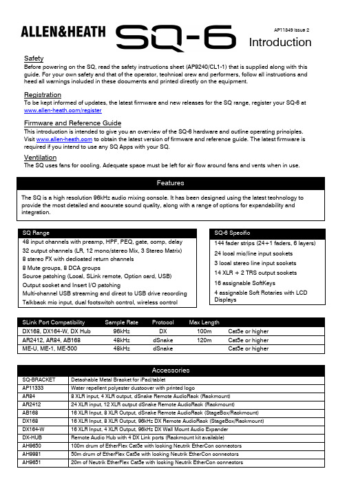
IntroductionSafetyBefore powering on the SQ, read the safety instructions sheet (AP9240/CL1-1) that is supplied along with this guide. For your own safety and that of the operator, technical crew and performers, follow all instructions and heed all warnings included in these documents and printed directly on the equipment. RegistrationTo be kept informed of updates, the latest firmware and new releases for the SQ range, register your SQ-6 at /registerFirmware and Reference GuideThis introduction is intended to give you an overview of the SQ-6 hardware and outline operating principles. Visit to obtain the latest version of firmware and reference guide. The latest firmware is required if you intend to use any SQ Apps with your SQ.VentilationThe SQ uses fans for cooling. Adequate space must be left for air flow around fans and vents when in use.FeaturesThe SQ is a high resolution 96kHz audio mixing console. It has been designed using the latest technology to provide the most detailed and accurate sound quality, along with a range of options for expandability and integration.AP11349 Issue 2AccessoriesSQ-BRACKET Detachable Metal Bracket for iPad/tabletAP11333 Water repellent polyester dustcover with printed logoAR84 8 XLR input, 4 XLR output, dSnake Remote AudioRack (Rackmount) AR2412 24 XLR input, 12 XLR output dSnake Remote AudioRack (Rackmount)AB168 16 XLR Input, 8 XLR Output, dSnake Remote AudioRack (StageBox/Rackmount) DX168 16 XLR Input, 8 XLR Output, 96kHz DX Remote AudioRack (StageBox/Rackmount) DX164-W 16 XLR Input, 4 XLR Output, 96kHz DX Wall Mount Audio Expander DX-HUB Remote Audio Hub with 4 DX Link ports (Rackmount kit available) AH9650 100m drum of EtherFlex Cat5e with locking Neutrik EtherCon connectors AH9981 50m drum of EtherFlex Cat5e with locking Neutrik EtherCon connectors AH965120m of Neutrik EtherFlex Cat5e with locking Neutrik EtherCon connectorsSLink Port Compatibility Sample Rate Protocol Max LengthDX168, DX164-W, DX Hub 96kHz DX 100m Cat5e or higher AR2412, AR84, AB168 48kHz dSnake 120mCat5e or higher ME-U, ME-1, ME-50048kHzdSnakeCat5e or higherSQ Range48 input channels with preamp, HPF, PEQ, gate, comp, delay 32 output channels (LR, 12 mono/stereo Mix, 3 Stereo Matrix) 8 stereo FX with dedicated return channels 8 Mute groups, 8 DCA groupsSource patching (Local, SLink remote, Option card, USB) Output socket and Insert I/O patchingMulti-channel USB streaming and direct to USB drive recording Talkback mic input, dual footswitch control, wireless controlSQ-6 Specific144 fader strips (24+1 faders, 6 layers) 24 local mic/line input sockets 3 local stereo line input sockets 14 XLR + 2 TRS output sockets 16 assignable SoftKeys4 assignable Soft Rotaries with LCD DisplaysLocal Mic/Line Inputs Local Stereo Line Inputs Talkback Mic Input Local XLR OutputsLocal TRS Jack OutputsAES Digital OutputMono/Dual Footswitch Connection Mains Power Input and Switch I/O Port - Option CardMulti-format multi-channel digital audioUSB-B PortConnection to a computer for multi-channel audio and MIDI I/O Network Port Connect to a router for network/wireless controlSLink PortFor connection to Allen&Heath remote audio racks, including AB, AR and DX ranges, as well as the ME personal monitoring systemTouch Screen, Screen Select Keys and Screen EncoderView processing and access the routing and setup menus using keys below. Touch to select a parameter and use the rotary to adjust values.Fader Strips and Layer Select Keys6 layers of 24 faders provide 144 assignable strips for access to any combination of channels, returns,masters and DCAs. Each strip has fader, mute, select and PAFL keys, peak and signal meter.Ident StripLCD displays show channel name and colour for each of the 24 strips. Press the‘View’ key to see secondary information such as input source.Channel(Pre/HPF/Gate/Comp)Physical controls for the selected channel. Preamp, HPF frequency, Gate threshold, Comp threshold.Channel (PEQ/GEQ)Physical controls for the selected channel. EQ band select keys and parametric controls. Use the ‘Fader Flip’ key to present selected mix GEQ on faders. Pan ControlMaster Strip and Mix Select KeysPress a blue ‘Mix’ key to present its sends on the 24 faders and its master on the master fader strip. Select ‘LR’ to work with the main LR mix and channel faders.FX Send Select KeysPress a blue ‘FX’ key to present its sends on the 24 faders and its master send on the master fader strip. Headphone Output and Level Control Main MeterDisplays the LR Mix or selected PAFL signal level.Talk KeyMomentary or latching switch for the talkback microphone.SQ-Drive PortRecord/play audio direct to/from a USB drive. Transfer scene, show and library data using a USB key. Update SQ firmware.ST3 Input3.5mm stereo jack input, can be used for connection to an external background music device.Pre Fade and Assign KeysHold ‘Pre-Fade’ and press ‘Sel’ to toggle channels pre or post fade to the mix. Hold ‘Assign’ and press ‘Sel’ to route channels to the selected mix.CH to All Mix KeyPress and hold to present all sends to mixes for the currently selected channel. The ident strip displays mix names. Copy/Paste/Reset KeysUsed to copy, paste or reset processing blocks or channel parameters.Library KeyOpens different libraries to enable save and recall of presets for channel/mix/FX processing.Assignable SoftKeysUse Setup screen to assign functions such as mutes, tap tempo, scene recall, SQ-Drive control and more.Assignable EncodersUse Setup screen to assign functions for quick access to often used parameters.i. Power off any connected amplifiers or powered speakers. ii. Navigate to the ‘Home’ screen and select ‘Shut Down’ iii.Switch off the unit using the push switch (27).Press a blue ‘LR’, ‘Mix’ or ‘FX’ Key to present send levels for the selected Mix on the 24 Fader Strips. Use the Layer Keys (2) to move through the 6 layers of faders and adjust individual levels. The Master strip (7) controls the master send level of the selected Mix/FX.Select a strip by pressing the green ‘Sel’ Key on a Fader Strip (2) or the Master Strip (7).The physical controls (4), (5) and (6) can now be used to adjust parameters for the selected strip.Go to the ‘Processing’ screen to see an overview of the processing for the selected strip.Tap on any part of the processing to see a detailed view, then touch a parameter on-screen and use the touch screen encoder (1) to adjust.Mute Keys are illuminated when a strip is muted.By default, PAFL (Pre/After Fade Listen) Keys allow you to route one channel at a time to the PAFL bus/Phones output. PAFL settings can be changed in the ‘Setup’ screen.Mix sends set to ‘Post Fade’ follow the LR send levels. To toggle channels between ‘Pre Fade’ and ‘Post Fade’ for the selected Mix, hold the ‘Pre Fade’ Key and use ‘Sel’ Keys.To assign or un-assign a strip from the currently selected mix, hold the ‘Assign’ Key and use ‘Sel’ Keys.Pressing and holding the ‘CH to All Mix’ Key will display the send levels for the currently selected strip across the main fader strips.Press the ‘FX’ Key to see and adjust FX engines.Use the ‘Library’ Key (17) to recall FX types and presets - change parameters by selecting on-screen and using the touch screen encoder.FX busses 1 to 4 (8) send to FX engines 1 to 4 by default.FX Return channels can be routed to Mixes in the same way as stereo input channels.Hold the ‘Copy’ Key and press an ‘In’ Key (4) (5), a ‘Sel’ Key (2) (7), to copy parameters.Hold the ‘Paste’ Key and press a ‘Sel’ Key (2) (7) to paste the copied processing to another channel. Hold the ‘Reset’ Key and press an ‘In’ Key (4) (5), a ‘Sel’ Key (2) (7), or on-screen to reset parameters.A ‘Scene’ is used to store or recall a mix. A ‘Show’ comprises multiple scenes and all settings. Press the ‘Scenes’ Key to access the list of scenes in the current show.Use a combination of scene filters and ‘Safes’ to decide which settings/parameters/strips are affected when a scene is recalled.i. Connect power lead (27).ii. Connect input sources using (20), (21) and (22).iii. Connect outputs (23) and (24) to amplifiers, speakers or line level inputs on other equipment. iv. If required, connect digital I/O such as AudioRacks or Computers using (25), (28), (29) and (31). v. If you are using a footswitch, connect this (26). vi. Switch on the SQ using the push switch (27).vii.Power on any connected amplifiers or powered speakers.To reset all mix, parameter and routing settings go to the ‘Scenes’ screen (1), then press and hold the ‘Reset Mix Settings’ button. This will ‘zero’ the desk without deleting saved scenes or libraries.To check or alter patching, go to the ‘I/O’ screen (1) and use the matrix to patch from Local/Digital Inputs to SQ input channels, and to patch SQ outputs [LR/Mix/Group/Matrix/DirectOut] to Local/Digital Outputs.Balanced mono/stereo inputs Mic or line level XLR 1=Gnd, 2=+, 3= -ST1 and ST2 Inputs Line level ¼” TRS Jack Tip= +, Ring= -, Sleeve=GndST3 Input Line level 3.5mm Jack Tip=Left, Ring=Right, Sleeve=Gnd Balanced XLR Outputs Line level XLR 1=Gnd, 2= +, 3= -Balanced Jack Outputs Line level ¼” TRS Jack Tip= +, Ring= -, Sleeve=GndSLink RJ45/EtherCON. Use Cat5e or higher. Refer to individual expansion unit instructions.AES Stereo Digital Output Digital XLR Use 110Ω AES CableRear USB Connection USB-B, Conforms to USB 2.0 standardNetwork Connection RJ45, Use Cat5e or higherFootswitch ¼” TRS (dual) or TS (mono) JackThere are many support resources available through our website including user guides, knowledgebase articles and access to the Allen & Heath Digital Community.For local language support, please contact the Allen & Heath distributor for your region.Limited One Year Manufacturer’s WarrantyAllen & Heath warrants the Allen & Heath -branded hardware product and accessories contained in the original packaging ("Allen & Heath Product”) against defects in materials and workmanship when used in accordance with Allen & Heath's user manuals, technical specifications and other Allen & Heath product published guidelines for a period of ONE (1) YEAR from the date of original purchase by the end-user purchaser ("Warranty Period").This warranty does not apply to any non-Allen & Heath branded hardware products or any software, even if packaged or sold with Allen & Heath hardware.Please refer to the licensing agreement accompanying the software for details of your rights with respect to the use of software/firmware (“EULA”).Details of the EULA, warranty policy and other useful information can be found on the Allen & Heath website: /legal.Repair or replacement under the terms of the warranty does not provide right to extension or renewal of the warranty period. Repair or direct replacement of the product under the terms of this warranty may be fulfilled with functionally equivalent service exchange units.This warranty is not transferable. This warranty will be the purchaser’s sole and exclusive remedy and neither Allen & Heath nor its approved service centres shall be liable for any incidental or consequential damages or breach of any express or implied warranty of this product.Conditions of WarrantyThe equipment has not been subject to misuse either intended or accidental, neglect, or alteration other than as described in the User Guide or Service Manual, or approved by Allen & Heath. The warranty does not cover fader wear and tear.Any necessary adjustment, alteration or repair has been carried out by an authorised Allen & Heath distributor or agent. The defective unit is to be returned carriage prepaid to the place of purchase, an authorised Allen & Heath distributor or agent with proof of purchase. Please discuss this with the distributor or the agent before shipping. Units returned should be packed in the original carton to avoid transit damage.DISCLAIMER: Allen & Heath shall not be liable for the loss of any saved/stored data in products that are either repaired or replaced.Check with your Allen & Heath distributor or agent for any additional warranty information which may apply. If further assistance is required please contact Allen & Heath Ltd.Any changes or modifications to the equipment not approved by Allen & Heath could void the compliance of the product and therefore the user’s authority to operate it.。
cognitiveRadio[1]答辩PPT
![cognitiveRadio[1]答辩PPT](https://img.taocdn.com/s3/m/a11dbd16f7ec4afe05a1df36.png)
5
Cognitive Radio Overview
Software Radio
Programmable Wideband Wideband RF Processor(s) A/D-D/A* Conversion
HF LVHF VHF-UHF Cellular
PCS Indoor & RFLAN VHDRBaseband Modem
Back End Control
Equalizer Algorithm
Software
Antenna
Hardware
RF
Modem
INFOSEC
Baseband
User Interface
Secure Downloads, Pro-Active Radio Resource Management
contains RKRL j
Micro-world j := {<Frame>}*
<Frame>
<Handle><Model><Body><Context><Resource-specification>
Syntax
<Root><Source><Time><Place> <Resources><Depth><Breadth><Sub-Elements><Sub-Frames>
RF IF
Bits
Bits
Aux
Aux or
Aux
CT
Fill
PT
BB
Air
I/O
QPSK
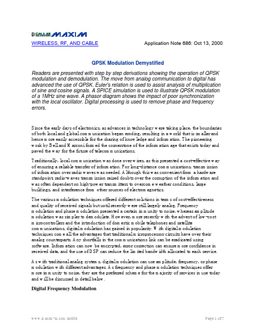
WIRELESS, RF, AND CABLE Application Note 686: Oct 13, 2000QPSK Modulation DemystifiedReaders are presented with step by step derivations showing the operation of QPSK modulation and demodulation. The move from analog communication to digital has advanced the use of QPSK. Euler's relation is used to assist analysis of multiplication of sine and cosine signals. A SPICE simulation is used to illustrate QPSK modulationof a 1MHz sine wave. A phasor diagram shows the impact of poor synchronizationwith the local oscillator. Digital processing is used to remove phase and frequency errors.Since the early days of electronics, as advances in technology were taking place, the boundaries of both local and global communication began eroding, resulting in a world that is smaller and hence more easily accessible for the sharing of knowledge and information. The pioneeringwork by Bell and Marconi formed the cornerstone of the information age that exists today and paved the way for the future of telecommunications.Traditionally, local communication was done over wires, as this presented a cost-effective wayof ensuring a reliable transfer of information. For long-distance communications, transmissionof information over radio waves was needed. Although this was convenient from a hardware standpoint, radio-waves transmission raised doubts over the corruption of the information and was often dependent on high-power transmitters to overcome weather conditions, large buildings, and interference from other sources of electromagnetics.The various modulation techniques offered different solutions in terms of cost-effectivenessand quality of received signals but until recently were still largely analog. Frequency modulation and phase modulation presented a certain immunity to noise, whereas amplitude modulation was simpler to demodulate. However, more recently with the advent of low-cost microcontrollers and the introduction of domestic mobile telephones and satellite communications, digital modulation has gained in popularity. With digital modulation techniques come all the advantages that traditional microprocessor circuits have over their analog counterparts. Any shortfalls in the communications link can be eradicated using software. Information can now be encrypted, error correction can ensure more confidence in received data, and the use of DSP can reduce the limited bandwidth allocated to each service. As with traditional analog systems, digital modulation can use amplitude, frequency, or phase modulation with different advantages. As frequency and phase modulation techniques offer more immunity to noise, they are the preferred scheme for the majority of services in use today and will be discussed in detail below.Digital Frequency ModulationA simple variation from traditional analog frequency modulation (FM) can be implemented by applying a digital signal to the modulation input. Thus, the output takes the form of a sine wave at two distinct frequencies. To demodulate this waveform, it is a simple matter of passing the signal through two filters and translating the resultant back into logic levels. Traditionally, this form of modulation has been called frequency-shift keying (FSK).Digital Phase ModulationSpectrally, digital phase modulation, or phase-shift keying (PSK), is very similar to frequency modulation. It involves changing the phase of the transmitted waveform instead of the frequency, these finite phase changes representing digital data. In its simplest form, a phase-modulated waveform can be generated by using the digital data to switch between two signals of equal frequency but opposing phase. If the resultant waveform is multiplied by a sine wave of equal frequency, two components are generated: one cosine waveform of double the received frequency and one frequency-independent term whose amplitude is proportional to the cosine of the phase shift. Thus, filtering out the higher-frequency term yields the original modulating data prior to transmission.This is difficult to picture conceptually, but mathematical proof will be shown later.Quadraphase-Shift ModulationTaking the above concept of PSK a stage further, it can be assumed that the number of phase shifts is not limited to only two states. The transmitted "carrier" can undergo any number of phase changes and, by multiplying the received signal by a sine wave of equal frequency, will demodulate the phase shifts into frequency-independent voltage levels.This is indeed the case in quadraphase-shift keying (QPSK). With QPSK, the carrier undergoes four changes in phase (four symbols) and can thus represent 2 binary bits of data per symbol. Although this may seem insignificant initially, a modulation scheme has now been supposed that enables a carrier to transmit 2 bits of information instead of 1, thus effectively doubling the bandwidth of the carrier.The proof of how phase modulation, and hence QPSK, is demodulated is shown below.The proof begins by defining Euler's relations, from which all the trigonometric identities can be derived.Euler's relations state the following:which gives an output frequencyby any phase-shifted sine wave.To prove this,Thus, the above proves the supposition that the phase shift on a carrier can be demodulated into a varying output voltage by multiplying the carrier with a sine-wave local oscillator and filtering out the high-frequency term. Unfortunately, the phase shift is limited to two quadrants;a phase shift of /2. Therefore, to accurately decode phase shifts present in all four quadrants, the input signal needs to be multiplied by bothsinusoidal and cosinusoidal waveforms, the high frequency filtered out, and the data reconstructed. The proof of this, expanding on the above mathematics, is shown below. Thus,A SPICE simulation verifies the above theory.Figure 1A shows a block diagram of a simple demodulator circuit. The input voltage, QPSK IN, is a 1MHz sine wave whose phase is shifted by 45°, 135°, 225°, and then 315° every 5µs.Figures 2 and 3 show the "in-phase" waveform, Vi, and the "quadrature" waveform, V q, respectively. Both have a frequency of 2MHz with a dc offset proportional to the phase shift, confirming the above mathematics.Figure 1B is the phasor diagram showing the phase shift of QPSK IN and the demodulated data.The above theory is perfectly acceptable, and it would appear that removing the data from the carrier is a simple process of low-pass filtering the output of the mixer and reconstructing the 4 voltages back into logic levels. In practice, getting a receiver local oscillator exactly synchronized with the incoming signal is not easy. If the local oscillator varies in phase with the incoming signal, the signals on the phasor diagram will undergo a phase rotation, its magnitude equal to the phase difference. Moreover, if the phase and frequency of the local oscillator are not fixed with respect to the incoming signal, there will be a continuing rotation on the phasor diagram.Therefore, the output of the front-end demodulator is normally fed into an ADC and any rotation resulting from errors in the phase or frequency of the local oscillator are removed in DSP.With the advances in monolithic silicon germanium (SiGe) technology, all of the above front-end circuitry can be integrated to reduce the problems outlined. A good example of how much of the front-end circuitry can be integrated is illustrated in the MAX2450, ultra-low-power quadrature modulator/demodulator IC. This is one of many devices from Maxim Integrated Products that incorporates the quadraphase shifter, the on-chip oscillator, and the mixer. Once the data has been demodulated, the output can be applied to a high-frequency dual-channel ADC (such as the MAX1002 or the MAX1003) before processing the signal in DSP.As the MAX2450 is designed to be used at an IF of 35MHz to 80MHz, RF signals up to2.5GHz can be downconverted using the MAX2411A. This is a high-frequencyup/downconverter with a low-noise amplifier (LNA) local oscillator, and it has access to the output of the LNA for image-reject filtering.Alternatively, an effective way of converting straight to baseband is using a direct-conversion tuner IC. The MAX2102 is designed to take RF inputs from 2150MHz and convert directly down to baseband I and Q signals, thus providing cost savings over multiple-stage devices. The above devices are part of the rapidly expanding RF chipsets from Maxim Integrated Products. With five high-speed processes, more than 70 high-frequency standard products, and 52 ASICs in development, Maxim is committed to being a major player in the RF/wireless, fiber/cable, and instrumentation markets.MORE INFORMATIONMAX1002:QuickView -- Full (PDF) Data Sheet (120k)-- Free Sample MAX1003:QuickView -- Full (PDF) Data Sheet (128k)-- Free Sample MAX2102:QuickView -- Full (PDF) Data Sheet (160k)-- Free Sample MAX2361:QuickView -- Full (PDF) Data Sheet (40k)-- Free Sample MAX2411A:QuickView -- Full (PDF) Data Sheet (144k)-- Free Sample MAX2450:QuickView -- Full (PDF) Data Sheet (120k)-- Free Sample。
600_electrical_engineering_books
這600本書幾乎包括了電氣工程專業的所有內容。
例如:電子學最基礎的《Circuit.Analysis.Theory.And.Practice.》(電路分析)、哈佛大學的經典教材《The.Art.of.Electronics》(電子學的藝術)、DSP.Facts.and.Equipment。
詳細書籍名:Wireless.Securit.PrivacyBest.Practices.and.Design.Techniques.Artech-Interference.Analysis.and.Reduction.for.Wireless.Systems.munications.works.munications.Network.Design._20-_20.Wiley._.Sons.802.11.Security.N.Fundamentals.Cisco.Press.eBookwork.Site.Surveying.and.Installation.Cisco.Press.Nov.2004.eBookA.First.Course.in.Corporate.Finance.b.in.Circuits.and.Electronics.munication.er_27s.Guide.to.Aspect.Ratio.Conversion.A.wavelet.tour.of.signal.processing.Mallat.S..draft_.2005.MNw.ponent.Modeling.Morgan.Kaufmann.eBook.-.LiB. Abstract.Harmonic.Analysis.of.Continuous.Wavelet.Transforms.Adaptive.Digital.Filters.Second.Edition.putational.Intelligence.Perspective.Adaptive_20Control_20Systems.Addison.Wesley._20-_20.RTP..Audio.and.Video.for.the.Internet.Advanced.Digital.Signal.Processing.and.Noise.Reduction.2nd.Edition.Advanced.Techniques.in.RF.Power.Amplifier.Design.works.Springer.eBook.Advanced_20Control_20Engineering.Advances.in.Fingerprint.Technology.Second.Edition.eBookworks.Artech.House.Publishers.Jun.2005.eBook. Aerials..Air.and.Spaceborne.Radar.Systems.An.Introduction.2001.WilliamAndrewPublishing.RR. munication.Systems.And.Their.Applications.Alternative.Breast.Imaging.Kluwer.Academic.Publishers.eBook.An.Introduction.To.Statistical.Signal.Processing.An.Introduction.to.Digital.Audio.An.Introduction.to.Pattern.Recognition.An_20Introduction_20to_20the_20Theory_20of_20Microwave_20Circuits_20_Kurokawa_. Analog.BiCMOS.Design.Practices.and.Pitfalls.Analog.Circuit.Design.Analog.Circuits.Cookbook.Analog.Integrated.Circuit.Design.Analog.and.Digital.Circuits.for.Electronic.Control.System.Applications..Analog_20And_20Digital_20Control_20System_20Design.Analysis.And.Design.Of.Analog.Integrated.Circuits.Analysis_20and_20Design_20of_20Integrated_20Circuit-Antenna_20Modules.Antenna_20Arraying_20Techniques_20In_20The_20Deep_20Space_20Network.Antenna_20handbook.rmation.Super.Skyways.Institute.of.Physics.Publishing.Feb.2004.eBook-DDU. Application.-.Specific.Integrated.Circuits.-.Addison.Wesley.Michael.John.Sebastian.Smith. munications.2002.Art.And.Business.Of.Speech.Recognition.Addison.Wesley.eBook.yout.Artech..Radio.Frequency.Integrated.Circuit.Design.Artech.House.GPRS.for.Mobile.Internet.rmation.theory.Asynchronous.Circuit.Design..Audel.Electrical.Course.for.Apprentices.and.Journeymen.eBook.Automated.Fingerprint.Identification.Systems..AFIS..Academic.Press.eBookAutomotive_20Computer_20Controlled_20Systems_20Diagnostic_20Tools_20And_20Techniques. Bandwidth.efficient.digital.modulation.in.deep.munications.ponents._.Hardware.-.I.CFS.ponents._.Hardware.-.II.CFS.Basic.Theory.and.Application.of.Transistors.Bebop.to.the.Boolean.Boogie.Bluetooth.Application.Developers.Guide.Bluetooth.Demystified.Bluetooth.Security.2004.BluetoothGuide.Broadband.Bible.John.Wiley.and.Sons.eBook.Broadband.Bringing.Home.the.Bits.Broadband.Microwave.Amplifiers.Artech.House.eBook-TLFeBOOK.Building.Financial.Models.McGraw-Hill.2004.works.with.802.11.eBook.C.Algorithms.for.Real._20-_20.time.DSP.1995.CAD_20of_20Microstrip_20Antennas_20for_20Wireless_20Applications.CDMA.Capacity.and.Quality.Optimization.CDMA.Mobile.Radio.Design.Artech.House.CDMA.RF.System.Engineering.CDMA.Systems.Capacity.Engineering.Artech.House.Publishers.eBook._20-_20.kB.CMOS.Analog.Circuit.Design.CMOS.Electronics.How.It.Works.How.It.Fails.yout.CMOS.Integrated.ADC.and.DAC.2ndEd..CMOS.PLL.Synthesizers.Analysis.and.Design.Springer.Nov.2004.eBook.-.LinG.CMOS.memory.circuits.CRC.Press.munications.Facility.Design.Handbook.CRC_20Press_20-_20Intelligent_20Control_20Systems_20Using_20Soft_20Computing_20Metho dologies.Cellular.Mobile.Radio.Systems.Designing.Systems.For.Capacity.Optimization.Circuit.-.techniques-for-low-voltage-high-speed-ADCs.Circuit.Analysis.Theory.And.Practice.Circuit.Design.for.RF.Transceivers.munications.Circuits.for.the.Hobbyist.Closed.Circuit.Television.Closing.The.Gap.Between.ASIC.and.Custom.Tools.And.Techniques.of.High.Performance.ASIC.Desig n.work.Test.and.Measurement.Handbook.works._20-_20.Fundamental.Concepts.-.McGraw.Hill.-.Leon-Garcia_.Widjaja. Communications.Receivers.DSP_.Software.Radios_.and.Design_.Third.Edition.Compact_20and_20Broadband_20Microstrip_20Antennas.Complete.Wireless.Design.Computer.Explorations.in.Signals.and.Systems.Computer.imaging.recipes.in.C.Myler.H.R._.Weeks.A.R..PH_.1993pi.T.munication.Consumer_27s.Guide.to.Cell.Phones.and.Wireless.Service.Plans.Continuous.-.Time.Active.Filter.Design.Control_20EngineeringGuide_20For_20Beginners.Coplanar_20Waveguide_20Circuits__20Components__20and_20Systems.Crane.R..Simplified.approach.to.image.processing.in.C.PH_.1997.T.ISBN.0132264161.DOE.Fundamentals.Handbook_.Electrical.Science.vol.1.DOE.Fundamentals.Handbook_.Electrical.Science.vol.2.DOE.Fundamentals.Handbook_.Electrical.Science.vol.3.DOE.Fundamentals.Handbook_.Electrical.Science.vol.4.DSP.Facts.and.Equipment.DSP.Realtime.Operating.Systems.for.Embedded.Systems.DSP.for.In.Vehicle.and.Mobile.Systems.Springer.eBook-YYePG.working.Devices._20-_20.Fourth.Edition.Data.Conversion.Handbook.Elsevier.eBook.-.LinG.Deep.Submicron.CMOS.Circuit.Design.Simulator.In.Hands.Delmar.Digital.Signal.Processing._20-_20.-Filtering.Approach.Delmar.Fiber.Optics.Technician_27s.Manual.2nd.Ed..Design.Of.Linear.RF.Outphasing.Power.Amplifiers.Artech.House.eBookNs.Springer.Sep.2005. Design.of.Analog.CMOS.Integrated.Circuits.Design_20of_20RF_20And_20Microwave_20Amplifiers_20And_20Oscillators..Designing.Analog.Chips.work.works.Developments.in.Speech.Synthesis.John.Wiley.Sons.Apr.2005.eBook._20-_20.LinG. Dictionary.of.Video.Television.Technology.Dielectric_20Resonator_20Antennas.Digital.Audio.Broadcasting.munication.Over.Fading.Channels.munications.Design.for.the.Real.World.Digital.Design.Fundamentals.Digital.Design.Principles.and.Practices.Digital.Electronics.Digital.Frequency.Synthesis.Demystified.Digital.Integrated.Circuits.wo02_8.munication.Digital.Logic.And.Microprocessor.Design.With.VHDL.Digital.Signal.Processing.Handbook.VK.Madisetti_DB.Williams_CRC.ing.C.bVIEW.Newnes.Jun.2005.eBook._20-_20.D DU.munications.Ieee.Digital.Switching.Systems.System.Reliability.and.Analysis.Digital.Synthesizers.and.Transmitters.for.Software.Radio.Springer.Jul.2005.eBook._20-_20.DDU. Digital.Systems.Engineering..Digital.Video.Quality.Vision.Models.and.Metrics.John.Wiley.and.Sons.Mar.2005.eBook._20-_20.D DU.Digital.Video.for.Dummies.Wiley..2003._.3Ed.Digital.image.processing._20-_20.B.Jahne.Digital.signal.Processing.Digitally.Assisted.Pipeline.ADCs.Theory.and.Implementation.Discovering.Bluetooth.Sybex.Discrete.Time.Signal.Processing._20-_20.Oppenheim.Distortion.Analysis.of.Analog.Integrated.Circuits.Distortion.in.rf.power.amplifiers.ebook._20-_20.lib.Duda.R.O._.Hart.P.E._.Stork.D.G..Pattern.classification.02ed._.Wiley.C.738s.EDGE.for.Mobile.Internet.ESD.In.Silicon.Integrated.Circuits.Electrical.Circuits.plante_CRC.Electrical._.Electronic.Principles._.Technology.-.0750665505.Newnes.John.Bird.Electrician_27s.Exam.Question.and.Answers.Electromagnetic_20Waves_20and_20Antennas.Electronics.for.Dummies.John.Wiley.and.Sons.eBook.-.LinG.Electronics.for.Hobbyists.1.Electronics.for.Hobbyists.2.Electronics.for.Hobbyists.3.Electronics.for.Hobbyists.4.Electronics.for.Hobbyists.5.Electronics.for.Hobbyists.6.Electronics.for.Hobbyists.7.work.Technologies.Springer.Sep.2004.eBook._20-_20.LinG. working.Engineer_27s.Mini.-._5bNotebook.-.555_5d.-.Timer.IC.Circuits.Engineer_27s.Notebook.II.A.Handbook.Of.Integrated.Circuit.Applications.-.Forrest.Mims. Engineering.Digital.Design.rmation.Theory.Error.control.coding..From.theory.to.practice.Sweeney.P..Wiley_2002.Essentials.of.Managing.Corporate.Cash.-.John.Wiley.Sons.Experimental.Approach.CDMA._.Interference.From.Architecture.Through.VLSI.Fast.Forward.MBA.in.Finance.Feedback.Amplifiers.Theory.and.Design.Feedback.Circuit.Analysis.Feedback.Linearization.of.RF.Power.Amplifiers.Feedbackcontroltheory.munication.Systems.Fiber.Optic.Sensors.Fiber.to.the.Home.The.New.Empowerment.Wiley.Interscience.Oct.2005.eBook._20-_20.LinG. Fibre.Channel.for.Mass.Storage._20-_20.Prentice.Hall.Fibre.Channel.for.SANs.Filter.Handbook.a.Practical.Design.Guide.-.S..Niewiadomski.Finance.for.Non.-.Financial.Managers.Financial.Engineering.Principles.A.Unified.Theory.Financial.Risk.Manager.Handbook.Wiley.Second.Edition.Financial.modeling.with.jump.processes.Finite_20Antenna_20Arrays_20and_20FSS.First.course.on.wavelets.Hernandez_.Weiss..CRC_.1996.T.ISBN.0849382742.Fixed.Broadband.Wireless.System.Design._20-_xxuss.For.Dummies.HDTV.For.Dummies.Nov.2004.eBook._20-_20.DDU.Fundamental_20Limitations_20In_20Filtering_20And_20Control.Fundamentals.Of.Electric.Circuits..Fundamentals.Of.RF.Circuit.Design.With.Low.Noise.Oscillators.munication.Fundamentals.of.Global.Positioning.System.Receivers.Fundamentals.of.Telecommunications.Fundamentals.of.wavelets..Theory_.algorithms_.and.applications.Goswami_.Chan..Wiley.T.319s. Fuzzy_20Control_20Systems_20-_20Design_20and_20Analysis.munications.works..Protocols.Terminology.and.Implementation.GSM.Switching.Services.and.Protocols.Getting.Started.As.a.Financial.Planner.Rev.and.Updated.Guide.To.Budgets.And.Financial.Management.Guide.To.Digital.Signal.Processing.HF_20Antenna_20Cookbook.HF_20Filter_20Design_20and_20Computer_20Simulation.Handbook.Of.Time.Series.Analysis_.Signal.Processing_.And.Dynamics.Handbook.of.Multisensor.Data.Fusion.puting.munications.works.Harjani.Design.Of.Modulators.For.Oversampled.Converters.Wang.-.1998.High.-.Speed.Signal.Propagation.Advanced.Black.Magic.Prentice.eBook-LiB.High.-.speed.Digital.Design.-.Johnson._.Graham.High.Frequency.Techniques.An.Introduction.to.RF.and.Microwave.Engineering.Wiley-IEEE.Press.. High_20Performance_20Control.IEE.Tutorial.Meeting.on.Digital.Signal.Processing.for.Radar.and.Sonar.Applications_.1990. IEEE.._20-_20..Telecommunications.Performance.Engineering.IEEE._20-_20.Adaptive.fuzzy.power.control.for.CDMA.mobile.radio.systems.IEEE._20-_work.Modeling_.Planning.and.Design.work.Design.Guide.IP.Routing.working_3b.Straight.to.the.Core.Ieee._20-_munication.Circuits.And.Systems.works.Springer.Sep.2005.eBook._20-_20.DDU. bVIEW.And.IMAQ.Vision.Prentice.eBook._20-_20.LiB.Image.Processing.in.C.Image.Recognition.and.Classification..algorithms-marcel.dekker.-.2002.-.isbn.0824707834.-.49. works.Newnes.Jul.2004.eBook._20-_20.DD U.Implementing.Bluetooth.in.an.Embedded.Device.Industrial.electronics.for.engineers_.chemists_.and.technicians.Industrial_20Control.Integrated.Electronics.Integrated.Fiber.Optic.Receivers.Buchwald.Intermodulation_20Distortion_20in_20Microwave_20and_20Wireless_20Circuits. Introduction.To.Error.Correcting.Codes.Introduction.To.Logic.Design.-.Shiva.S.G..-.M.Dekker.1998.2Ed.Introduction.To.Sound.Processing.work.Engineering.Introduction.to.03G_munications.Introduction.to.Airborne.Radar.Introduction.to.Bluetooth.Technology_.Market_.Operation_.Profiles_._.Services. Introduction.to.CPLD.and.FPGA.Design.Introduction.to.Fiber.Optics.Introduction.to.RF.Equipment.and.System.Design.Introduction.to.RF.Propagation.Wiley.Interscience.Sep.2005.eBook._20-_20.DDU. Introduction.to.Wireless.Local.Loop.Introduction_to_Wave_Propagation_Transmission_Lines_and_Antennas.John.Wiley.And.Sons.An.Introduction.To.Parametric.Digital.Filters.And.Oscillators.John.Wiley.And.Sons.Device.Modeling.For.Analog.And.RF.CMOS.Circuit.Design.John.Wiley.And.Sons.Digital.Logic.Testing.And.Simulation.John.Wiley._20-_20.Fundamentals.of.Digital.Television.Transmission.John.Wiley._20__20.Sons._20-_works.John.Wiley._20__20.Sons._20-_20.Mobile.and.Wireless.Design.Essentials.work.Design.Aug.2004.eBook._2 0-_20.DDU.John.Wiley.and.Sons.Multi.Carrier.and.Spread.Spectrum.Systems.works.Karu.J..Signals.and.systems_.made.ridiculously.simple.2001.L.T.ISBN.0964375214.Kay.S.M..Fundamentals.of.statistical.signal.processing...estimation.theory.PH.L.T.30.Ken.Martin.Digital.Integrated.Circuit.Design.300dpi.ponents.eBook.-.LiB. works.eBook._20-_20.LiB. Kluwer.Reuse.Methodology.Manual.for.System.-.on-a-Chip.Designs.3rd.Ed..LabVIEW.Digital.Signal.Processing.McGraw.Hill.Professional.May.2005.Layout.CMOS..Circuit.Design._.Li.Simulation.Baker._Boyce.-.1997.2.Linear_20Control_20System_20Analysis_20and_20Design_20Fifth_20Edition.Linear_20Optimal_20Control.Liquidity.Liabilities.Cash.Management.Balancing.Financial.Risks.Wiley.Low-Angle_Radar_Land_Clutter_-_Measurements_and_Empirical_Models.Lumped_20Elements_20for_20RF_20and_20Microwave_20Circuits.MPEG.7.Audio.and.Beyond.Audio.Content.Indexing.and.Retrieval.John.Wiley.and.Sons.Jan.2006. puter.Vision.Springer.Aug.2005.eBook._20-_20.DDU.McGraw.-.Hill.Teach.Yours.Electricity.and.ElectronicsEbook-FLY.McGraw.Hill.-.Principles.and.applications.of.Electrical.Engineering.McGraw.Hill.Financial.Analysis.Tools.and.Techniques.a.Guide.for.Managers.McGraw.Hill._20-_ponents.McGraw.Schaum_27s.Outlines.of.Digital.Signal.Processing.McGraw.Schaum_27s.Outlines.of.Signals._.Systems.McGraw._20-_20.Hill.-.Broadband.Crash.Course.-.2002.McGraw._20-_20.Hill.-.Wireless.A.to.Z.puter._20-_20._20T.266s_20.-.oriented.Approach.to.Pattern.Recognition.AP_.19 72.Microstrip_20Filters_20For_20RF_20Microwave_20Applications.Microwave_20Circuit_20Modeling_20Using_20Electromagnetic_20Field_20Simulation. Microwave_20Component_20Mechanics.Microwave_20Electronics_20Measurement_20and_20Materials_20Characterization. Microwave_20Resonators_20and_20Filters_20For_20Wireless_20Communication.Microwave_engineering_using_microstrip_circuits_.Microwaves.and.Wireless.Simplified.Artech.House.2nd.Edition.Apr.2005.Millimeter.-.wave.Integrated.Circuits.Springer.eBook-YYePG.Mixed.Signal.And.DSP.Design.Techniques.working._20-_20.John.Wiley._.Sons.-.IEEE.Press.munications.Engineering._20-_20.Theory.and.Applications_.Second.Edition. munications.Mobile.Location.Services.The.Definitive.Guide._20-_20.Prentice.Hall.works.Wiley._20-_20.eBOOK.Model.Based.Signal.Processing.Wiley.IEEE.Press.Oct.2005.eBook._20-_20.LinG.Modern.Antenna.Design.Jun.2005.eBook-DDU.munication.Circuits.Modern.Receiver.Front.Ends.Systems.Circuits.and.Integration.Wiley.Feb.2004.eBook-DDU. Modern.Signal.Processing.Modern_20Control_20Engeneering__203rd_20ed_5d._5bOgata_5d_5bPrentice_20Hall_5d. Morgan.Kaufmann.._20-_20..Digital.Video.And.Hdtv.Algorithms.And.Interfaces.2003.Multi.-.Standard.CMOS.Wireless.Receivers_.Analysis._.Design.Multicarrier.Techniques.for.04G_munications.Multivariable.Control.Systems.An.Engineering.Approach.Springer.eBook-TLFeBOOK.Nano.CMOS.Circuit.and.Physical.Design.Network.Calculus.A.Theory.of.Deterministic.Queuing.Systems.for.the.Internet.Networks_20and_20Devices_20Using_20Planar_20Transmissions_20Lines.Neural_20Systems_20For_20Control.New.technologies.for.WLAN.munications.Pocket.Book.Newnes.Guide.to.Television._.Video.Technology.Newnes.Radio.and.RF.Engineering.Pocket.Book.Newnes_20Industrial_20Control_20Wiring_20Guide.Next.Generation.Mobile.Systems.3G.and.Beyond.John.Wiley.and.Sons.May.2005.eBook._20-_20. DDU.Nixon_.Aguado..Feature.Extraction.and.Image.Processing.2002.Noise.In.Receiving.Systems.Nonlinear.Microwave.And.RF.Circuits.2nd.Edition.Nonlinear_20Microwave_20Circuit_20Design.ON.Analog.Integrated.Circuits.OReilly.Digital.Video.Hacks.May.2005.eBook._20-_20.DDU.OReilly.RFID.Essentials.Jan.2006.O_27Reilly._20-_20._20802._20-_works-.The.Definitive.Guide. Observers_20in_20Control_20Systems.Op.Amp.Applications..Op.Amps.Design.Application.and.Troubleshooting.Op.Amps.for.Everyone.Design.Reference.Operational.Amplifiers.Design.and.Applications.munications.Essentials.munications.Rules.of.Thumb.working.Handbook.Mcgraw._20-_20.Hill.Optical.System.Design.Optical.Through._20-_munications.Handbook.Optical.signal.processing.Vanderlugt.A..Wiley_.1991pi.L.T.180s.PEo.Optimal.Filtering.Optimal_20Control_20Linear_20Quadratic_20Methods.Optimal_20Sampled_20Data_20Control_20Systems.Optimizing.Wireless._20-_20.RF.Circuits.work.Handbook.Pattern.Classification.And.Learning.Theory.Lugosi.nguage.Processing.works.Polling_.Scheduling_.and.Traffic.Cont rol.munications.Phased.Array.Antenna.Handbook.Artech.House.Publishers.Second.Edition.eBook-kB.Phased_20Array_20Antennas_20Hansen_20R.C._20_Wiley_1998__ISBN_20047153076X__200dp i__T__504s__EE_.Photodetection._20__20.Measurement._20-_20.Maximizing.Performance.in.Optical.Systems. Practical.Analog.And.Digital.Filter.Design.Practical.Electronics.for.Inventors.Practical.FPGA.Programming.in.C.Prentice.Hall.PTR.Apr.2005.yout._20-_e.of.Stock.Lenses.Practical.Rf.Pcb.Design.Geoff.Smithson.Scanned.Practical.Rf.System.Design._20-_20.Egan.Practical_20Applications_20of_20Computational_20Intelligence_20for_20Adaptive_20Control. Practical_20Approach_20to_20Signals_20Systems_20and_20Control.Pragmatic.Introduction.to.Electronic.Engineering.0._v1_.works.John.Wiley.and.Sons.munication.system.simulation.with.wireless.applications._20-_20.Prentice.Hall. Principles.Of.Corporate.Finance.Principles.of.Asynchronous.Circuit.Design.-.A.Systems.Perspective.Principles.of.Digital.Transmission.With.Wireless.Applications.Principles.of.Sigma.Delta.Conversion.for.Analog.to.Digital.Converters.munication.Systems.eBook._20-_20.TLFeBOOK. Programmable.Digital.Signal.Processors.Architecture.Programming_.and.Applications. munication.System.Design.QoS.in.Integrated.03GNetworks.2002.Quantitative.Finance.for.Physicists.An.Introduction.Queueing.Theory.With.Applications.to.Packet.Telecommunication.Springer.eBook._20-_20.YYePG. RDS..The.Radio.Data.System.RF-Microwave_20Circuit_20Design_20for_20Wireless_20Applications.ponents.and.Circuits.munications.munications.RFID.Field.Guide.Deploying.Radio.Frequency.Identification.Systems.Feb.2005.eBook._20-_20.LiB. RFID.For.Dummies.Mar.2005.eBook._20-_20.LinG.RFID.Sourcebook.Prentice.Hall.PTR.RFID._20-_20.Read.My.Chips_.RF_20__20Microwave_20Radiation_20Safety_20Handbook.RF_20and_20Microwave_20Wireless_20Systems.Radar.Systems_.Peak.Detection.and.Tracking.Radar.Technology.Encyclopedia._20-_20.1998.Radar_20Principles.munication.and.Sensor.Applications.Radio.Engineers_27.Handbook._20-_20._2001e_20-_20.-.d.-.Terman.Radio.Frequency.Circuit.Design.Radio.Frequency.Transistors.Radio.Shack.-.Getting.started.in.electronics.Radio.Shack.Engineer_27s.Mini.-._5bNotebook.T.52s_5d.Radio._.Electronics.Cookbook.Radio_20Frequency_20and_20Microwave_20Communication_20Circuits.Radiometric.Tracking.Techniques.for.Deep.Space.Navigation.Radiosity.and.realistic.image.synthesis.Cohen.M.F._.Wallace.J.R..AP_.1995.Real.802.11.Security.Wi._20-_20.Fi.Protected.Access.And.802.11i.Addison.Wesley.eBook-LiB. Real.Analog.Solutions.for.Digital.Designers.Real.World.Digital.Audio.Peachpit.Press.No05._20v.200.Real._20-_pression--Techniques.And.Algorithms.Rf.Cmos.Power.Amplifier._20-_20.Ebook.Kluwer.Inter.Hella._.Ismall.Risk.Management.And.Capital.Adequacy.McGraw.Hill.SIP.Demystified.MUNICATIONS.HANDBOOK.munication.Engineering.eBook._20-_20.EEn.Satellite.Handbook.working.Principles.and.Protocols.John.Wiley.and.Sons.Oct.2005.eBook._20-_20.DDU. Schaums.Outline.Of.Theory.And.Problems.Of.Electric.Circuits.eBook.Secrets.of.RF.Circuit.Design._.Third.Edition.Securing.and.managing.WLAN.Shannon._20-_20.TheoryComm.munication.Fundamentals.of.RF.System.Design.and.Application. Signal.Analysis.Alfred.Mertins.Signal.Analysis.Time.Frequency.Scale.and.Structure.RL.Allen_ls.Signal.Detection.and.Estimation.munications.Handbook._20-_20.CRC.Press.-.2005.Signal.analysis.wavelets.filter.banks-Mertins.A..Wiley_.1999.Signals.And.Systems.Signals._20__20.Systems.with.MATLAB.Applications._20-_20.Orchard.Publications. munications.Sliding_20Mode_20Control_20in_20Engineering.Smart.Antennas.CRC.Press.Jan.2004.eBook-DDU.Some.Design.Aspects.on.RF.CMOS.LNAs.and.Mixers.Sonet.or.SDH.Demystified.Space._20-_20.Time.Coding.John.Wiley.And.Sons.eBook.Space._20-_munications.Specification.of.the.Bluetooth.System.Spectrum.Wars.Speech.Coding.Algorithms.Foundation.and.Evolution.of.Standardized.Coders.Wiley.eBook._20-_2 0.KB.works.Speech.Separation.By.Humans._20__20.Machines.Springer.eBook._20-_20.YYePG.Stability_20Analysis_20of_20Nonlinear_20Microwave_20Circuits.pression.to.Advanced.Video.Coding.IEEE.Standard.Handbook.of.Audio.and.Radio.Engineering.Standard.Handbook.of.Video.and.Television.Engineering_.4th.ed.Starting.Electronics.-.Elsevier.-.3rd.Edition.-.2005.Statistical.and.Adaptive.Signal.Processing.Supervised.and.Unsupervised.Pattern.Recognition.Synthesis.and.optimization.of.DSP.algorithms.Constantinides_.Cheung_.Luk..Kluwer_.2004.T.144s_20Bayesian.Approach.to.Image.Interpretation.Kopparapu_.Desai..Kluwer_.2002.T.181s_20Wavelets_.with.applications.in.signal.and.image.processing.Bultheel.A..2002.T.212s_20Brandwood..Fourier.transforms.in.radar.and.signal.processing.2003.T.359s_20Mann.S..Intelligent.image.processing.Wiley_.2002.T.406s_20Dudgeon.D._.Mersereau.R._.Merser.R._.Multidimensional.Digital.Signal.Processing.199 5.T.548s_20Ballard.D.H._.Computer.vision.Brown.C.M..PH_.1982.ISBN.0131653164.T.621s_20Image.analysis.and.mathematical.morphology.Serra.J..AP_.1982.300dpi.CsIp.TAB.Electronics.Guide.to.Understanding.Electricity.and.Electronics.eBook.-.EEn.Telecom.Crash.Course.Telecom.Dictionary.Telecommunication.Circuit.Design._20-_20.Second.Edition.Telecommunications.Essentials.CHM.Telecommunications.Regulation.Teletraffic.Engineering.Handbook.The.Art.and.Science.of.Analog.Circuit.Design.The.Art.of.Electronics.02ed.munications.Professional..A.Guide.for.Engineers.and.Managers. working.The.Engineer_27s.Guide.to.Decoding._.Encoding.The.Engineer_27s.Guide.to.Standards.Conversion.The.Great.Telecom.Meltdown.Artech.House.Jan.2005.eBook._20-_20.LiB.works.munications.Handbook.The.Mobile.Radio.Propagation.Channel._20-_20.Second.Edition.-.Wiley.The.Personal.Finance.Calculator.McGrawHill.munication.Applications.Handbook.The.Telecommunications.Handbook.The.Wireless.Data.Handbook._20-_20.Fourth.Edition.Thetrated.dictionary.of.electronics.Troubleshooting.Analog.Circuits.US.Navy._20-_20.Digital.Data.Systems.Ultra.Wideband.Radio.Technology.ing.Coded.Signals.Understanding.Cellular.Radio.munications.Understanding.Digital.Signal.Processing.Understanding.Digital.Terrestrial.Broadcasting.MAZ._20-_20.Artech.House. munications.Understanding.Telephone.Electronics.Understanding_20Microwaves_20_Scott_.rmation.Retrieval.IRM.eBook._20-_20.YYePG.Video.Demystified.A.Handbook.For.The.Digital.Engineer.munications.Voice.Over.802.11.W._20-_20._20for.03G_works.munications.System.Waveguide_20Handbook.Wavelets.For.Kids.A.Wavelets.For.Kids.B.Wideband.TDD.WCDMA.for.the.Unpaired.Spectrum.John.Wiley.Sons.May.2005.eBook._20-_20.Lin G.Wiley.-.Essentials.of.Financial.Analysis.Wiley._20-_works_.IP.and.the.Internet.-.Protocols_.Design.and.Operation.Wiley._20-_20.Digital.Image.Processing.WK.Pratt.-.Third.Edition.2001.munication.Systems._20-_20.Prentice.Hall.PTR.munication.Technologies.munication.Technology.munications.Wireless.Data.Demystified.McGraw.Hill.eBook._20-_20.LiB.Wireless.Data.Technologies.Reference.Handbook.John.Wiley.and.Sons.Wireless.Foresight.Scenarios.of.the.Mobile.World.in.2015.John.Wiley.and.Sons.eBook._20-_20.Li B.Wireless.Internet.Telecommunications.Artech.House.Publishers.eBook._20-_20.YYePG. working.with.ANSI._20-_20._2041__20-_20.-.Second.Edition.works.First._20-_20.Step..2005.munication.Systems.Springer.Verlag.Telos.Sep.2004.ISBN0387227849. Wireless.Technology.Protocols.Standards.and.Techniques.Young_.Gerbrands_.van.Vliet..Fundamentals.of.image.processing.Delft.U._.1998.T.11._5bT.270s_5dJohnson.D.H._.Wise.J.D..Fundamentals.of.electrical.engineering.1999._5bT.498s_5dGustafsson.F..Adaptive.Filtering.and.Change.Detection.Wiley_.2000._Delmar__20Modern_20Control_20Technology--Components_20__20Systems_20_2nd_20Ed._. dsp.algorithms.for.programmers.eWiley.Mobile.Fading.Channels._20-_20.-Modelling_.Analysis._.Simulation.electronics_20technician_20volume_201_20-_20safety.electronics_20technician_20volume_202_20-_20administration.electronics_20technician_20volume_203_20-_20communications_20systems.electronics_20technician_20volume_204_20-_20radar_20systems.electronics_20technician_20volume_206_20-_20digital_20data_20systems.electronics_20technician_20volume_207_20-_20antennas_20and_20wave_20propagation. low.power.asynchronous.DSP.numerical_20methods_20in_20electromagnetics.operational.amplifiers.-.2nd.edition.practical_aspects_of_feedback_control.structure.and.interpretation.of.signals.and.systems.下載地址:/file/f5ddfade86600_electrical_engineering_books.rar。
TL-WA850RE 300Mbps 通用 Wi-Fi 扩展器 使用说明书
TL-WA850RE300Mbps Universal Wi-Fi Range ExtenderCOPYRIGHT & TRADEMARKSSpecifications are subject to change without notice. is a registered trademark of TP-LINK TECHNOLOGIES CO., LTD. Other brands and product names are trademarks or registered trademarks of their respective holders.No part of the specifications may be reproduced in any form or by any means or used to make any derivative such as translation, transformation, or adaptation without permission from TP-LINK TECHNOLOGIES CO., LTD. Copyright ©2015 TP-LINK TECHNOLOGIES CO., LTD.All rights reserved.FCC STATEMENTThis equipment has been tested and found to comply with the limits for a Class B digital device, pursuant to part 15 of the FCC Rules. These limits are designed to provide reasonable protection against harmful interference in a residential installation. This equipment generates, uses and can radiate radio frequency energy and, if not installed and used in accordance with the instructions, may cause harmful interference to radio communications. However, there is no guarantee that interference will not occur in a particular installation. If this equipment does cause harmful interference to radio or television reception, which can be determined by turning the equipment off and on, the user is encouraged to try to correct the interference by one or more of the following measures:∙Reorient or relocate the receiving antenna.∙Increase the separation between the equipment and receiver.∙Connect the equipment into an outlet on a circuit different from that to which the receiver is connected.∙Consult the dealer or an experienced radio/ TV technician for help.This device complies with part 15 of the FCC Rules. Operation is subject to the following two conditions:1) This device may not cause harmful interference.2) This device must accept any interference received, including interference that maycause undesired operation.Any changes or modifications not expressly approved by the party responsible for compliance could void the user’s authority to operate the equipment.Note: The manufacturer is not responsible for any radio or tv interference caused by unauthorized modifications to this equipment. S uch modifications could void the user’s authority to operate the equipment.FCC RF Radiation Exposure StatementThis equipment complies with FCC RF radiation exposure limits set forth for an uncontrolled environment. This device and its antenna must not be co-located or operating in conjunction with any other antenna or transmitter.“To comply with FCC RF exposure compliance requirements, this grant is applicable to only Mobile Configurations. The antennas used for this transmitter must be installed to provide a separation distance of at least 20 cm from all persons and must not be co-located or operating in conjunction with any other antenna or transmitter.”CE Mark WarningThis is a class B product. In a domestic environment, this product may cause radio interference, in which case the user may be required to take adequate measures.Canadian Compliance StatementThis device complies with Industry Canada license-exempt RSS standard(s). Operation is subject to the following two conditions:(1)This device may not cause interference, and(2)This device must accept any interference, including interference that may cause undesired operation of the device.Cet appareil est conforme aux norms CN R exemptes de licence d’Industrie Canada. Le fonctionnement est soumis aux deux conditions suivantes:(1)cet appareil ne doit pas provoquer d’interférences et(2)cet appareil doit accepter toute interférence, y compris celles susceptibles de provoquer un fonctionnement non souhaité de l’appareil.Industry Canada StatementComplies with the Canadian ICES-003 Class B specifications.Cet appareil numérique de la classe B est conforme à la norme NMB-003 du Canada.This device complies with RSS 210 of Industry Canada. This Class B device meets all the requirements of the Canadian interference-causing equipment regulations.Cet appareil numérique de la Classe B respecte toutes les exigences du Règlement sur le matériel brouilleur du Canada.Korea Warning Statements당해무선설비는운용중전파혼신가능성이있음.NCC Notice & BSMI Notice注意!依據低功率電波輻射性電機管理辦法第十二條經型式認證合格之低功率射頻電機,非經許可,公司、商號或使用者均不得擅自變更頻率、加大功率或變更原設計之特性或功能。
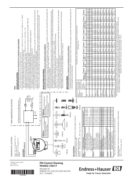
Radio Frequency (RF) 系列产品说明书
–
+
+
external load
–
4...20 mA loop
supply
Option (1): Prepared to connect FM Approved remote display type FHX40 from Endress+Hauser
ቤተ መጻሕፍቲ ባይዱ
Option (2): Interconnection with FM Approved Service Interface Commubox FXA193 with ToF-Cable from Endress+Hauser
–40 °C/–40 °F to +200 °C/392 °F –40 °C/–40 °F to +350 °C/662 °F –60 °C/–76 °F to +400 °C/752 °F depends on type –60 °C/–76 °F to +280 °C/536 °F –60 °C/–76 °F to +400 °C/752 °F
FMR232-
Notes.
Intrinsically safe installation Intrinsically safe (entity), Class I, Div. 1, Groups A, B, C, D, Hazardous Location Installation.
1. Control room equipment may not use or generate over 250 Vrms. 2. Use FM Approvals Entity-Approved intrinsic safety barrier with Voc or Vt £ Vmax, Isc or It £ Imax, Ca ³ Ci + Ccable, La ³ Li + Lcable
Detection of the Intrinsic Size of Sagittarius A through Closure Amplitude Imaging (include
a r X i v :a s t r o -p h /0404001v 1 31 M a r 2004Detection of the Intrinsic Size of Sagittarius A*through Closure Amplitude ImagingGeoffrey C.Bower,1∗Heino Falcke,2Robeson M.Herrnstein,3Jun-Hui Zhao,4W.M.Goss,5,Donald C.Backer 11Astronomy Department &Radio Astronomy Laboratory,University of California,Berkeley,CA 94720,USA 2Radio Observatory Westerbork,ASTRON,P.O.Box 2,7990AA Dwingeloo,The Netherlands 3Department of Astronomy,Columbia University,Mail Code 5246,550West 120th St.,New York,NY 10027,USA 4Harvard-Smithsonian Center for Astrophysics,60Garden Street,MS 78,Cambridge,MA 02138,USA 5National Radio Astronomy Observatory,Array Operations Center,P.O.Box O,Socorro,NM 87801,USA ∗To whom correspondence should be addressed;E-mail:gbower@.We have detected the intrinsic size of Sagittarius A*,the Galac-tic Center radio source associated with a supermassive black hole,showing that the short-wavelength radio emission arises from very near the event horizon of the black hole.Radio observations with the Very Long Baseline Array show that the source has a size of 24±2Schwarzschild radii at 7mm wavelength.In one of eight 7-mm epochs we also detect an increase in the intrinsic size of 60+25−17%.These observations place a lower limit to the mass density of SgrA*of1.4×104solar masses per cubic astronomical unit.Sagittarius A*(Sgr A*)is the compact,nonthermal radio source in the Galactic Center associated with a compact mass of4×106M⊙(1,2,3).It is the best established and closest supermassive black hole candidate and serves as the prime test case for the black hole paradigm.Emission at radio,near-infrared,and X-ray wavelengths traces processes in the environment of the event horizon(4,5,6,7,8,9).High resolution radio imaging of Sgr A*can ultimately distinguish between the many different models for the emission,accretion and outflow physics of the source as well as provide an important test of strong-field gravity(10).Sgr A*has been a target of such observations for the past30years(11).Its intrinsic size and structure have remained obscured,however,because radio waves from Sgr A*are scattered by turbulent interstellar plasma along the line of sight(12).The scatter-broadened image of Sgr A*is an ellipse with the major axis oriented almost exactly East-West and a quadratic size-wavelength relation.The turbulent plasma is parametrized with a power-law of turbulent energy density as a function of length scale with outer and inner scales that correspond to the scale on which turbulence is generated and damped,respectively.Scattering theory predicts that the scatter-broadened image will be a Gaussian when the inner length scale of the turbulent medium is larger than the longest baseline of the observing interferometer(13).Addition-ally,the scatter-broadened image size will scale quadratically as a function of wavelength. In the case of Sgr A*,the longest interferometer baseline used in our analysis b max∼2000 km corresponds to a length scale in the scattering medium D scattering/D source×b max∼25 km,where D source=8kpc is the distance from Sgr A*to the Earth and D scattering=100 pc is the distance from Sgr A*to the scattering screen(12).This scale is much less than the predicted and measured values of the inner scale,which fall in the range102to105.5km(14,15).The amplitude of turbulence in the Galactic Center scattering screen is∼2−3orders of magnitude greater than what is seen in the next most powerful scat-tering region,NGC6334B(16),however,suggesting that the Galactic Center case may be atypical.The presence of strong scattering has pushed observations to shorter and shorter wavelengths where scattering effects decrease and intrinsic source structure may dom-inate,creating a deviation from the measured size-wavelength law.On the basis of extensive observations with the National Radio Astronomy Observatory’s Very Long Baseline Array(VLBA),L98measure the index of the size-wavelength power-law to be α=1.99±0.03(17).L98also claim a deviation from the scattering law in the minor axis at7mm wavelength(43GHz),implying an intrinsic size of72Schwarzschild radii (R s)(18).Unfortunately,precise measurements of the size of Sgr A*are seriously hampered by calibration uncertainties related to the variable antenna gain and atmospheric opacity at the low antenna elevations necessary to observe Sgr A*from the northern hemisphere. Closure amplitudes have been used to constrain the size of Sgr A*with VLBI observations at3.4mm(19).The closure amplitude does not rely on calibration transfer from another source as traditional imaging methods do and is independent of all station-dependent amplitude errors.This method does not,however,eliminate baseline-dependent errors such as variable decorrelation(which also influence conventional calibration and imaging techniques).The closure amplitude is conceptually related to the closure phase,a more well-known quantity which is also independent of station-based gain errors.The principle drawback of closure amplitude analysis for simple source structures is the reduction in the number of degrees of freedom relative to a calibrated data set.The number of independent data points for a7-station VLBA experiment is reduced by a factor14/21.Additionally,the closure amplitude method can not determine the absoluteflux density for the source. These shortcomings are more than offset by the confidence that the result gives through its accurate handling of amplitude calibration errors.We describe here the analysis of new and archival VLBA data through closure am-plitude and closure phase quantities.We analyze3new experiments including data at 1.3cm,6new experiments including data at0.69cm,as well as10experiments from the VLBA archive including data at6,3.6,2.0,1.3,0.77,0.69and0.67cm wavelength.Observations and Initial Data ReductionSix new observations were made with the VLBA as part of our Very Large Arrayflux density monitoring program(20).Three observations were made in each of two sepa-rate epochs in July/August2001and April/May2002(STable1).In thefirst epoch, observations at1.3cm and0.69cm were interleaved over5hours.In the second epoch, observations were obtained only at0.69cm in order to maximize the signal to noise ra-tio(SNR)of thefinal result.All observations were dual circular polarization with256 Mbits/sec recording rate.We also analyzed a number of experiments from the VLBA archive over the wavelength range of6.0cm to0.67cm(STable1).The experiments BS055A,B and C were those analyzed by L98.The experiment BB113was previously analyzed(21).Initial data analysis was conducted with the NRAO Astronomical Imaging Processing System(22).Standard fringe-fitting techniques were employed to remove atmospheric and instrumental delays from the data(SOM text).High SNR fringes were detected for most stations on the compact source NRAO530(J1733-1302),indicating the overall quality of the data.Due to the relatively larger size of Sgr A*,fringes were obtained for a subset of5to8stations(STable1).Data were then averaged over wavelength and time for each experiment.The quality of thefinal result is dependent upon the visibility averaging time.The longer the averaging time,the higher the SNR of the closure amplitude calculation(23).On the other hand, as the averaging time approaches the phase decorrelation time,the closure amplitudes cease to be accurate.It is not necessary,however,to determine the best averaging time precisely,since neither of these effects is a strong function of time(23).The results that we give are for an averaging time of30seconds,but wefind that for averaging times of 15to120seconds the estimated intrinsic size of Sgr A*does not differ by more than10% (SOM text).No amplitude calibration was applied at any stage.The averaged data were then written to textfiles for analysis by our own analysis programs,external to AIPS.Closure Amplitude and Closure Phase Analysis of a Single GaussianWe form the closure amplitude from the measured visibilities and average the closure amplitudes over time.Closure amplitudes were averaged over scans,which were5to15 minutes in duration.The code uses the scatter in the closure amplitudes before averaging to determine the error in the closure amplitude.Only independent closure amplitudes were formed(24).We selected visibility data only with station elevations>10◦to reduce sensitivity to phase decorrelation,which is more significant at low elevations.We also excluded data at (u,v)distances greater than25Mλat6.0cm,50Mλat3.6cm,150Mλat2.0cm and 1.3cm,and250Mλat0.69cm.These sizes are comparable to the expected size of Sgr A*at each wavelength.Visibility amplitudes beyond the cutoffwere indistinguishable by inspection from noise.This(u,v)-distance limit reduced sensitivity to the noise bias or station-dependent differences in the noise bias.Results were not strongly dependent onthe value of this cutoff.Model visibilities for each baseline and time datum were computed for an elliptical source of a givenflux density S0,major axis size x,minor axis size y and position angle φ.In addition,a noise bias was added in quadrature to each model visibility.Our model visibility amplitude(squared)on baseline ij is thenA2ij=S20e−D0((u′ij x)β−2+(v′ij y)β−2)+N2ij,(1)where D0=2(π)2,N ij is the noise bias,and u′ij and v′ij are baseline lengths in log2units of wavelength in a coordinate system rotated to match the position angleφ.Model closure amplitudes were then formed from these model visibilities.We determine the best-fit parameters using a non-linearfitting method that minimizesχ2between the model and measured closure amplitudes(SFig.1,STable2).Wefind the reducedχ2for the amplitudesχ2A≈1for all experiments.In the case of an image produced by interstellar electron scattering on baselines longer than the inner scale of turbulence,βis the power-law index of electron densityfluctuations (13).The parameterβis related to the exponentαof the scattering law(size∝λα)as β=α+2,allowing an independent check of theλ2law(13,14,15).For the case of the Galactic Center scattering we expectβ=4,in which case Equation1is a Gaussian function and x and y are the FWHM in the two axes.Allowingβto be unconstrained in ourfits,wefindβ=4.00±0.03,which is consistent with the expectation of scattering theory(SFig.3).All remaining analysis is conducted with the assumption thatβ=4.The introduction of the noise bias to the model changes our calculation from a pure closure amplitude to a noise-biased closure amplitude.We found that our results did not require that we consider the noise bias as dependent on station or time(SOM text).Thus, we chose N ij(t)=N0because it is simpler computationally and has a smaller number ofindependent parameters.Errors in the model parameters were determined by calculatingχ2for a grid of models surrounding the solution andfitting constantχ2surfaces(SFig.2).Monte Carlo simula-tionsfind confidence intervals that are smaller by a factor of two than determined from the χ2analysis,suggesting that the dominant sources of error are baseline-based errors such as phase decorrelation,which were not included in the Monte Carlo simulations(SOM text).Closure phases were formed,averaged and analyzed in a manner similar to the closure amplitudes.We tested the closure phases against the hypothesis that they are all zero. This hypothesis is the case for a single elliptical Gaussian and other axisymmetric struc-tures with sufficiently smooth brightness distributions.An axisymmetric disk is a notable exception to this hypothesis since it induces ringing in the transform plane.The reduced χ2for this hypothesisχ2φ≈1for all experiments(STable2),indicating no preference for multiple components,non-axisymmetric structure or disk-like structure.Although the solutions for a single Gaussian component are sufficiently accurate,we did search the parameter space for two component models.To do this,we performed a minimization ofχ2with respect to closure amplitude and closure phase jointly.The reducedχ2for these models was roughly equal to the values for the single Gaussian component despite the addition of several degrees of freedom.We also calculated upper limits to theflux densities of secondary components that are in the range2-10%,typically (SFig.4,STable2).The absence of any improvement indicates that a single Gaussian component is sufficient and the simplest model of the data.This absence is particularly significant for the cases whereχ2>1and suggests,as noted before,that the results are dominated by closure errors rather than improperly modeled structure.Scattering Law and Intrinsic SizeWe determined the size of the major and minor axes of Sgr A*for each experiment(Fig.1 and2,STable2).The major axis is oriented almost exactly East-West.The major axis size is measured much more accurately than the minor axis size because of the poorer North-South resolution of the array.All major axis measurements at1.3and0.69cm are larger than the scattering size determined by L98(25)and the new scattering size that we determine below,although the difference is statistically significant in only one epoch at0.69cm.Minor axis measurements are distributed about the scattering result and no one differs significantly from the expected result.The L98scattering law is adequate for the minor axis measurements as a function of wavelength(Fig.3).All the measured minor axis sizes agree with the scattering law to better than3σ.The data are also consistent with a constant position angle of78.0+0.8−1.0 deg withχ2ν=2.2forν=6degrees of freedom.We determinefits to the major and minor axis sizes as a function of wavelength using subsets of the data with a minimum wavelengthλmin of2.0cm,1.3cm,0.6cm and0.3 cm(STable3).The lastfit includes the3.4mm circular Gaussianfits of for the major axis only(19).There are twofits for each subset,allowingαto vary andfixingα=2.χ2νis less than3for the minor axis case withλ≥0.6cm,confirming that the solution is adequate forα=2.The major axis data,however,are discrepant from the L98and the new scattering law (Fig.3).All of the7mm results fall above the L98scattering law.Two of these points are significantly different at greater than3σ.The L98scattering law predicts a size of690µarcsec at0.69cm,which is∼7σfrom the measured size(712+4−3µas)and smaller than any of the measured sizes(Fig.2).An attempt tofit a scattering law withαmajor=2toall data withλ>0.6cm givesχ2ν=24for6degrees of freedom,demonstrating that the hypothesis can be strongly rejected.In fact,the1.35cm major axis size is also discrepant with the best-fitαmajor=2scattering law,givingχ2ν=5.6for3degrees of freedom.We consider two alternative models for our resuls:case A,the scattering power-law exponentαmajor is not exactly2;or,case B,intrinsic structure in Sgr A*is distorting the size-wavelength relation at short wavelengths.For case A,wefind adequate solutions for all data at wavelengths≥0.3cm with αmajor=1.96±0.01.The result is clearly discrepant with scattering theory which re-quiresβ=4and marginally discrepant with our determination of the scattering theory parameterβ=4.00±0.03(SFig.3),since scattering theory predicts thatα=β−2.For case B,we determine a new scattering law from observations withλ≥2.0cmthat is even less than that of andαmajor=2.This solution has a scale parameterσ1cmmajorL98,increasing the discrepancy at short wavelengths.Removing this new scattering law in quadrature gives an intrinsic size of0.7±0.1mas at1.35cm,0.24±0.01mas at0.69 cm and0.06±0.05mas at0.35cm(Table1).On the basis of the disagreement betweenβandα,we reject case A and claim that we have determined the size of intrinsic structure in Sgr A*at1.35and0.69cm.The two cases predict substantially different sizes at20cm.For the major axis case A predicts541±2mas while case B predicts595±3.The20.7cm(ν=1450MHz) major axis size624±6mas measured with the VLA A-array(26)is discrepant with both of these cases,although more strongly with case A.These measurements are particularly difficult since the source is only partially resolved in the A-array:the synthesized beam is about2.6×0.9arcsec oriented North-South.Additionally,extended structure in the Galactic Center makes estimation of the size strongly dependent on the estimate of the zero-baselineflux density.We attempted to verify the20cm size with analysis of three VLA A-array observa-tions at21.6cm obtained originally for polarimetry(8).Results for each of the three experiments were similar and dominated by systematic errors that make an estimate of the intrinsic size difficult.We were unsuccessful at analyzing these experiments with our closure amplitude technique,possibly due to the poor resolution of Sgr A*and inability of our code to handle the large number of stations.In any case,the reliability of ampli-tude calibration of the VLA at20cm reduces the need for closure amplitude analysis. We imaged all baselines and measured the totalflux density of Sgr A*byfitting a two-dimensional Gaussian to the central3′′.For all epochs,wefind an error in the totalflux density of10mJy.We determined the size byfitting in the(u,v)plane with the totalflux densityfixed and with a minimum cutoffin(u,v)distance.For values of the totalflux density that range from−1σto+1σand for a minimum(u,v)distance from20to120 kλ,wefind that the major axis size varies systematically from580to693mas.The minor axis is very poorly constrained.We estimate the size from the mean of these results as 640±40mas.We consider this to be a more reasonable estimate of the error in the size of Sgr A*than previously given.This size is consistent at<1σwith case B and∼1.5σwith case A,favoring slightly detection of the intrinsic size.Although all minor axis data are adequatelyfit withαminor=2,we can check the consistency of our results by estimating intrinsic sizes for this axis in the same way. The minor axis sizes show the same trend as the major axis sizes:smaller than the L98scattering law at long wavelengths and larger than the L98scattering law at short wavelengths(Fig.3).Using the solution forαminor=2andλ≥2.0cm,we estimate intrinsic sizes of1.1±0.3mas at1.35cm and0.26±0.06mas at0.69cm.These are comparable to the sizes determined for the major axis.For the case of unconstrained power-law indexfit to all data,wefindαminor=1.85+0.06,marginally consistent with no−0.06intrinsic source.Changes In the Source Size with TimeAt0.69cm,the only measurement deviating significantly from the mean result is inµas while the mean result the major axis for BB130B.The BB130B result is770+30−18µas.We note that the greatest deviation in is712+4−3µas giving a difference of58+30−19the0.69cm position angle also occurs for BB130B,although the difference is significant only at the2σlevel.Any such deviation would indicate a non-symmetric expansion or a non-symmetric intrinsic source size.We can estimate the change in the size of the intrinsic source between BB130B and the mean size by subtracting in quadrature the case B scattering size from each.As stated above,the mean result implies an intrinsic size ofmas.Thus, 0.24±0.01mas.The intrinsic size implied by the BB130B result is0.38+0.06−0.04the growth in major axis size is0.14+0.06mas in the N-S direction.We cannot associate−0.04this change in structure with aflux density change.This maximum in the size comes ∼10days before detection of an outburst at0.69cm with the VLA(20).The following epoch,BB130C,occurs only two days before this outburst but shows no deviation from the mean size,although the size is particularly poorly determined in this case.The Interstellar Scattering ScreenThe image of a scattered source is created by turbulent plasma along the line of sight. The minimum time scale for the scattered image to change is the refractive time scale, the time in which the relative motions of the observer,turbulent plasma and background source lead to the background source being viewed through a completely different region of the interstellar plasma.The refractive time scale for Sgr A*is∼0.5λ2y cm−2given a relative velocity of100km s−1(13).At our longest wavelength for VLBA observations,6cm,then the time scale is20y.At our shortest wavelength of7mm,the time scale for refractive changes is3months.Our observations are distributed over a much larger time frame than three months,implying that the mean result may be affected by refractive changes.Two subsets of the archival data have much smaller span,however.The BS055experi-ments cover6.0to0.69cm in1week and the BL070and BB113experiments cover6.0cm to0.67cm in3months.These data sets include all of the2.0cm and longer wavelength data.If we compare the0.7cm size,we see that it is larger in these quasi-simultaneous experiments than in the mean of all experiments and also larger than the expectation ofthe new scattering law.Wefind0.69cm major axis sizes of728+16−11µas and713+12−9µasfor BS055C and BL070B,respectively,both larger than the mean size of712+4−3µas(STa-ble2).We conclude that if refractive effects are altering the short wavelength results, then their effect is to reduce the deviation from the scattering law,not enhance it.DiscussionOur results allow us to probe the mechanisms responsible for accretion,outflow and emission in the vicinity of the black hole.We can compare the measured7mm intrinsic major axis size of24R s and its dependence on wavelength with expected values(Fig.4). The intrinsic size of the major axis decreases with wavelength and is best-fit with a power-law as a function of wavelength with indexαintrinsic=1.6±0.2.Wefind for the minor axis a similar valueαintrinsic=2.1±0.5.Assuming that the source is circularly symmetric and using the meanflux density of1.0Jy at7mm(20),we compute a brightness temperature T b=1.2×10¹⁰× λThe wavelength-dependent size of Sgr A*now unambiguously shows that the source is stratified due to optical depth effects.We rule out models in which the emission originates from one or two zones with simple mono-energetic electron distributions(27). These models predict a size which is constant with wavelength and is larger than our measured size.The results are well-fit by a multi-zone or inhomogeneous model,in which the size is equal to the radius at which the optical depth is equal to unity(28).In a jet model, declining magneticfield strength,electron density and electron energy density contribute to a size that becomes smaller with wavelength.A detailed jet model for Sgr A*predicts an intrinsic size of0.25mas at0.69cm and0.6mas at1.3cm(Fig.4)(29).Exact values and wavelength dependence are a function of a number of parameters including the relative contributions of the extended jet and the compact nozzle component of the jet. The jet model also predicts that the source should be elongated with an axial ratio of4:1. The apparent measured symmetry in the deconvolved sizes in each axis,however,does not imply that the intrinsic source is symmetric.For example,an elongated intrinsic source that is oriented at45degrees to the scattering axis will produce equal deconvolved sizes in each axis.Modeling of the closure amplitudes with a complete source and scattering model is necessary to determine the elongation for the most general case.The thermal,high accretion rate models such as Bondi-Hoyle accretion(30)and ad-vection dominated accretionflows(31)require T e∼109K,which overpredicts the size in each axis by a factor of3.This disagreement confirms the elimination of these models on the basis of the polarization properties of Sgr A*(9).On the other hand,the radiatively inefficient accretionflow(RIAF)model(32)has a lower accretion rate and higher T e,com-patible with the polarization and with this measurement.The RIAF model also predicts an inhomogeneous electron distribution consistent with a size that reduces with decreasingwavelength.Both the RIAF model and the jet model are similar in the electron energy distribution and magneticfield distribution required to produce the observedflux density within the observed size.These models differ principally in the relative contribution of thermal electrons to emission in the submillimeter region of the spectrum.Extrapolating our size-wavelength relation to longer wavelengths,we estimate a size at2cm of130R s with a characteristic light travel time of85minutes.This is comparable to the shortest time scale for radio variability detected,2hours,during which the2.0cm radioflux density changed by20%(8).The smooth nature of the spectrum from90cm to7mm,suggests that our size-wavelength relation holds over that entire range(33).Our relation implies a size<2R s at1.3mm,comparable to the size of the event horizon.The decrease of the source size with wavelength cannot continue much farther due to thefinite size of the central object itself.In the millimeter and submillimeter, however,the spectral index rises(34),indicating that there may be a break in the size-wavelength relation.Ultimately,the size of the event horizon can be viewed as setting a limit on the wavelength of the peak emission.The strong break in the spectrum between the submillimeter and the NIR may correspond to the wavelength at which the source size becomes comparable to the event horizon.Even with a weaker dependence of size on wavelength,the light travel time scale at millimeter wavelengths is a few minutes, comparable to the shortest time scale observed at X-ray and NIR wavelengths.This coincidence suggests that the brightflares observed in at higher energies(7,5,6)are related to the submillimeter part of the spectrum and come from the vicinity of the black hole.The proximity of the millimeter emission indicates that emission at this and shorter wavelengths will be subject to strong light bending effects,providing a unique probe of strong-field general relativity(10,35).The size-wavelength relation also implies that the black hole mass must be containedwithin only a few Schwarzschild radii.Radio proper motion measurements require that Sgr A*must contain a significant fraction if not all of the compact dark mass found in the Galactic Center(36,37,38).Using conservatively only our7mm size and the lower limit of the Sgr A*mass of4×105M⊙,wefind that the mass density in Sgr A*has to be strictly aboveρ•>1.4×10⁴M⊙AU−3.The dynamical lifetime of a cluster of objects with that density would be less than1000years,making Sgr A*the most convincing existing case for a massive black hole(39).References and Notes1.F.Melia,H.Falcke,Annual Rev.Astron.Astrophys.39,309(2001).2.A.M.Ghez,et al.,Astrophys.J.Lett.586,L127(2003).3.R.Sch¨o del,et al.,Astrophys.J.596,1015(2003).4.H.Falcke,et al.,Astrophys.J.499,731(1998).5.R.Genzel,et al.,Nature425,934(2003).6.A.M.Ghez,et al.,Astrophys.J.Lett.601,L159(2004).7.F.K.Baganoff,et al.,Nature413,45(2001).8.G.C.Bower,H.Falcke,R.J.Sault,D.C.Backer,Astrophys.J.571,843(2002).9.G.C.Bower,M.C.H.Wright,H.Falcke,D.C.Backer,Astrophys.J.588,331(2003).10.H.Falcke,F.Melia,E.Agol,Astrophys.J.Lett.528,L13(2000).11.W.Goss,R.Brown,K.Lo(2003).Astron.Nachr.,Vol.324,No.S1(2003),SpecialSupplement”The central300parsecs of the Milky Way”,Eds.A.Cotera,H.Falcke, T.R.Geballe,S.Markoff.zio,J.M.Cordes,Astrophys.J.505,715(1998).13.R.Narayan,J.Goodman,Mon.Not.R.Astron.Soc.238,963(1989).14.P.N.Wilkinson,R.Narayan,R.E.Spencer,Mon.Not.R.Astron.Soc.269,67(1994).15.K.M.Desai,A.L.Fey,Astrophys.J.Supp.133,395(2001).16.A.S.Trotter,J.M.Moran,L.F.Rodriguez,Astrophys.J.493,666(1998).17.K.Y.Lo,Z.Q.Shen,J.H.Zhao,P.T.P.Ho,Astrophys.J.Lett.508,L61(1998).18.We assume for Sgr A*a black hole mass of4×106M⊙and a distance of8.0kpc(2).The latter implies that0.1mas=0.8AU=1.1×1013cm.Together,these quantities imply a Schwarzschild radius R s=2GM/c2=1.2×1012cm=0.08AU=0.01mas.19.S.S.Doeleman,et al.,Astron.J.121,2610(2001).20.R.Herrnstein,J.-H.Zhao,G.C.Bower,W.M.Goss(2004).Astron.J.,in press.21.G.C.Bower,D.C.Backer,R.A.Sramek,Astrophys.J.558,127(2001).22.E.W.Greisen,Information Handling in Astronomy-Historical Vistas(2003),pp.109–+.23.A.E.E.Rogers,S.S.Doeleman,J.M.Moran,Astron.J.109,1391(1995).。
- 1、下载文档前请自行甄别文档内容的完整性,平台不提供额外的编辑、内容补充、找答案等附加服务。
- 2、"仅部分预览"的文档,不可在线预览部分如存在完整性等问题,可反馈申请退款(可完整预览的文档不适用该条件!)。
- 3、如文档侵犯您的权益,请联系客服反馈,我们会尽快为您处理(人工客服工作时间:9:00-18:30)。
Radio Ad Filtering with Machine LearningMichael HolmesJosh JonesAdam FeldmanApril 17, 2003 IntroductionOur group explored an application of machine learning techniques to the binary classification of audio samples. The learned binary classification is intended to indicate whether a given sample is taken from music or from another type of audio signal (such as commercials or DJ talking).The datasets used for learning and evaluating this classifier consist of pairs of audio samples and their correct classification. The audio samples were obtained by digitally recording two different Internet radio stations – WREK and 99x. This method enabled the convenient acquisition of a large quantity of suitable audio data in digital format. These recordings were then broken into fixed-length chunks (samples). Each sample was transformed using Mel Frequency Cepstral Coefficients (MFCCs) in order to generate feature vectors.Once the feature vectors were generated, a random subset of data was used as a training set. The system to be trained was an SVM classifier. Several different kernels were experimented with (see results). The classification output from the SVM was used to train an HMM. This allowed accuracy and confidence information, as well as other data (such as time series data), to be considered in classifying a sample.This problem is interesting because it would allow for several applications. For example, many radio stations turn up the volume of their advertisements, which can be an inconvenience, to say the least. Therefore, a successful classifier could be used to monitor the start of commercials, and adjust the volume accordingly. Another application would be to serve as a“station changer”, allowing a listener to automatically change stations to ensure that music is always being played. Thus, a listener could supply a list of favorite stations that could be scrolled through whenever a commercial begins. Further, constant sampling across all the stations could help ensure that a station is chosen on which a song has recently started (as opposed to constantly tuning to stations for the tail ends of songs).Although existing research has focused on attempting to classify audio samples in various ways, little work has focused directly on music/non-music discrimination. Our learning task specifically requires determining what is integral to music, versus other kinds of sounds. This is a subtle, but significant difference between our project and the reference work we located. Most previous work has been on speech/music or genre discrimination. As an example of how this difference can influence system design decisions, notice that features that may be very useful for making certain kinds of distinctions between audio samples may not be useful for making other kinds of distinctions. For example, it might require a much more complicated decision to distinguish pure music from speech, speech with music in the background, effects noises, etc. than to simply distinguish music from speech. We also consider this project to be interesting and worthy of exploration because, to this point, no finished product with the capabilities we envision has been produced. Whether this is because no one has succeeded in enabling a machine to discriminate between music and non-music (by employing machine learning techniques or through other means), or simply because the technology has not been appropriately adapted to be useful in these contexts, it is clear that there is still progress to be made in this area.Prior WorkThe decision to use an SVM to produce initial classification confidences was based on a search of relevant literature detailing existing work on audio sample classification. Although little of this work focused directly on music/non-music classification, we considered it likely that techniques successful in some audio classification tasks would enjoy similar success when applied to our task. In particular, previous work shows SVMs to be superior to boosting for classification of audio samples into 16 distinct categories [1]. A number of additional studies confirm the applicability of SVM learning to this domain area [2, 5]. One other technique, “Nearest Feature Line” (NFL) was also described in several works, and appears in some cases within the audio classification domain to be superior to SVMs in both training time and accuracy of the resulting classifier [3,4]. The general principle behind NFL learning is to classify new instances by calculating the distance in feature space between the feature vector to be classified and a line between each possible pairing of training points within each class. The classification chosen is then whichever class contains the pair of training points generating the line in feature space from which the new example has minimum distance. In this way, it is similar to other memory-based methods. However, due to our greater familiarity with SVMs, the availability of high-quality software implementing SVM learning, and the existence of research leading to good results using SVMs for audio classification, we decided upon the use of SVM learning for this project. A potential avenue for future work could involve the implementation of a system similar to the one designed in this project, instead using NFL. Then, a direct comparison would be possible in the context of this task, with the possibility of producing interesting results that contrast the capabilities of the two techniques. But, such a comparison is outside the scope of this work.Most previous audio classification work has not incorporated time series information in any principled way. Scheirer and Slaney [7] implemented a music/speech discriminator that used 2.4-second window averages to boost performance on a frame-by-frame basis. However, this technique is rather ad hoc. We decided to incorporate time series information in Bayesian style through an HMM. Further, because the SVM output can be looked at as a measure of confidence in the classification, we developed a modification to normal HMM inference that uses the degree of confidence in the classification at each time step. This is in some sense similar to the hybrid HMM/neural network approach of [8], but their system used neural networks to change the probability table of observations given state at each time step, while our approach was to use the SVM to measure our belief in the observation, keeping the state/observation probability table constant throughout.The majority of previous work in audio classification has involved some form of Mel Frequency Cepstral Coefficients (MFCCs), which are a form of frequency spectrum adapted to the human perception of pitch. Two papers [4, 9] specifically contrast MFCCs with other audio features, and find that MFCCs perform favorably. This, combined with the availability of open source MFCC extractors, was the basis of our decision to use MFCC feature vectors in this work.ExperimentsOur first step was to gather a large amount of audio data. This was obtained by recording approximately two hours worth of Internet radio broadcasts from two different music stations. These audio files were then separated and regrouped into music and non-music segments, yielding approximately 600,000 samples.Since MFCCs are a well-established audio feature, we were able to use existing utilities to extract feature vectors from our audio samples. Specifically, we used the Edinburgh Speech Tools utility called sig2fv [10]. This gave us feature vectors containing twelve MFCCs for each 0.01-second interval. We wrote a utility to convert the output of sig2fv into a format useable by SVM lite [6], a well-regarded, open source, C-based SVM package. The data was then separated into a training set (5% or approximately 30,000 of the samples) and a test set (everything not in the training set). Because training times were prohibitively long, we decided against the normal 33%/67% splitting of the data. Several SVM kernels were tested, including linear, quadratic, cubic, quartic, etc. The cubic was found have best performance, and so was chosen for use in the time series system.Our initial approach to the incorporation of time series information was to create by hand a simple HMM and use the SVM classification as the HMM’s observed symbol at each time step. The HMM design is shown in Figure 1. The symbol M means music, and N means non-music.232.0)(,768.0)(==N M ππO=M O=N S=M0.9875 0.757 S=N 0.01250.243Figure 1: The HMM with transition probabilities, initial state probabilities, and observation probabilities.The numbers for the HMM were derived empirically from the raw data and the SVM results, i.e. 999947=MS=P because 99.9947% of the time a music sample is MS(=.0)'|πbecause 76.8% of the samples are music, followed by a music sample, 768M)(=.0S=MOP because the SVM classified 98.75% of the test music samples M=9875.0)|(=correctly.In order to appropriately test the HMM, it was necessary to obtain labeled data points in their original sequence. Previously all samples of a given type were grouped together, so only the set had to be labeled. We therefore cut an approximately 40-minute segment of the audio recordings and parsed it into music/non-music chunks, extracted ordered features and classifications from the chunks, and reassembled them into the full mixed sequence that included transitions between music and non-music. The fastest way to generate the sequential test set was to draw from only one radio station and not filter out 5% of data points that had been part of the training set. Time did not permit the creation of a more sophisticated sequential test set; however, 5% of the data points could not have had a large impact on overall performance.HMM inference was performed using the standard Viterbi algorithm [11], taking the final state of the most probable path for each time step as the state output for that step. The state output at each step was compared to the known label, and accuracies were computed for music and non-music classification. As we observed that music and non-music occur in large contiguous blocks, we added a domain-specific enhancement to the HMM: transitions out of a state were only allowed when the probability of being in the other state was higher than a threshold (0.9 to go from non-music to music, 0.55 to go from music to non-music; the reason for the asymmetry is that spurious SVM outputs are more common on non-music than on music samples).Finally, noting that the SVM output was not just a binary decision but the actual margin of each data point, we developed a modification to the HMM that used the SVM margin as a confidence measure in the correctness of the observation (M or N). This confidence measure was transformed into a probability that the observation is correct as follows. Since most margins had absolute value less than 1.5, the first confidence measure was either the absolute value of the margin if it was less than 1, or truncated to 1 if larger. This confidence measure alone was not a good estimate of the probability that the SVM gave the correct output; for example, a confidence of 0.2 that the sample is music does not mean that the probability of being non-music is 0.8. The key observation here is that a confidence of 0 should result in a 0.5 probability that the observation is correct, and a confidence of 1 should give a probability of 1. This leads to the formula)1(5.0)(confidence n Observatio Correct P +⋅=.So, for example, if the SVM classifies a sample as M with a certain confidence, then )1(5.0)(confidence M P +⋅= and )(1)(M P N P −=. Normally in Viterbi inference, the probabilities of the most probable path ending in state M would be updated as:)|(*),(*)(max )(,1M n Observatio P M j T j S P M S P t NM j t ====+. This assumes the observation is correct. We incorporate the possibility that the observation is incorrect by updating as follows:[][].)|(),()(max ))(1()|(),()(max )()(,1N n Observatio P M S T S P M Obs P M n Observatio P M j T j S P M Obs P M S P j jt j t N M j t ⋅⋅⋅=−+⋅⋅=⋅====+In other words, the new state probability is a linear combination of the normal Viterbi updates for each possible observation, weighted in proportion to the estimated probability that each observation was the correct one. We used the same state change thresholding in this modifiedHMM as we did in the normal HMM and again calculated accuracies for each class using the data labels.ResultsSeveral different SVM kernels were tested, with the results shown in Figure 2. The model dimensionality refers to the kernel used, ranging from a linear model (1), to a squared model (2), then a cubed model (3) and finally a quartic model (4). As the figure shows, the cubed model (3) has the best overall results. Specifically, this model correctly classified 98.8% of the tested music samples and 24.3% of all non-music samples, for an overall accuracy of 84.1%, which is higher than any other model in each measurement category. This was the basis of our decision to use the cubic model in the time series experiments.Figure 2: Test set accuracy for polynomial kernels of various dimensionalities.The SVM seemed adept at correctly classifying music samples, but performed very poorly on the non-music samples. Fortunately, this performance was increased greatly by the introduction of time series information. The accuracy results from the normal and modified HMMs are summarized with the original SVM accuracy in Table 1.Music Accuracy Non-Music Accuracy Overall Accuracy Static SVM 98.8% 24.3% 84.1% Normal HMM 88.6% 86.0% 88.0%Modified HMM 94.6% 73.5% 89.8%Table 1: Accuracy of normal and modified HMMs over the sequential test set. Note that the overall accuracy is not simply the average of the other two accuracies because there are more music than non-music data points.As can be seen, both types of HMM resulted in a relatively small decrease in the static music accuracy of 98.8%, while yielding very large increases over the 24.3% static non-music accuracy. Both HMMs outperformed the static SVM in overall accuracy, and the modified HMM performed 1.8% better than the normal HMM.ConclusionsAs the results of the experiment indicate, our method of classifying between music and non-music audio samples is successful. We have implemented a combination of SVM and HMM in order to provide the best possible chances of correctly identifying each sample. In this way, we have achieved an overall accuracy of 89.8%.Initially, MFCC is used to create a feature vectors for each audio sample. These feature vectors are then used to train a cubic SVM model. The SVM outputs a music or non-music margin, which we use for one-shot static sample classification, for normal HMM classification ina time series, and as a proto-confidence level in a modified HMM that uses a new version of Viterbi inference that takes into account uncertainty in the observation.We found that using the SVM alone produced very good results for classifying music samples (over 98%). However, the results of classifying non-music samples are significantly worse, at less than 25%. This averages to create an overall accuracy of approximately 84%. While this result is good on some level, the introduction of an HMM into the system yielded much better classifications. Specifically, the normal HMM had 88% accuracy, while our modified HMM technique yielded 90% accuracy. This is an especially interesting point, because the modified HMM technique is not at all domain specific, and the combination of a confidence-outputting classifier with the modified HMM technique could be a means of improving HMM performance in general.In the end, these results show promise, and indicate that these methods can be successful at classifying audio samples as music or non-music. Further, these results can possibly be improved upon through the addition of yet other techniques and/or making refinements to the techniques we employed. See below for possible future work and extensions to the project.Future WorkThere are several possible extensions to this project, some involving practical application of the classifier generated as the result of these experiments, and others focusing on improving the classifier itself by achieving a better understanding of applicable theories and methods within the context of binary audio classification. Ultimately, one goal would be to create a system for Internet radio listeners. This system would allow the user to define a series of favorite radio stations. Each radio station would be monitored for content – music vs. non-music. In this way,whenever a station is not playing music, it would be switched, in favor of a station that is playing music. Additionally, stations on which a song has recently started will be given priority over stations on which a song has been playing for longer (and therefore is nearer the end).Further, this concept could be extended, providing a similar service on television. In this domain, commercials are much more prone to increasing volume. Therefore, instead of changing the station, this system could be designed to automatically reduce the volume of the television. Taking this approach, as opposed to simply trying to constantly moderate the volume, would help prevent adjusting the volume from scene to scene in a given show or movie (which should not be interfered with).Another area of future interest involves different types of music. These techniques of discrimination should be examined in the context of classifying types of music (country vs. rap, for example). A motivation for this research would be to allow a listener to choose between channels based on type of music. Presumably in addition to removing commercials, this would ensure that a listener could listen to only the desired type of music, regardless of the fact that many stations play a variety of types.The general technique of combining a confidence-outputting classifier such as an SVM with the modified HMM inference is one that merits exploration in other domains. Testing in other areas and with other classifiers would lead to the discovery of whether this technique is a general improvement over regular HMMs or not.Any of these applications would require a broadening of the training set and improvement of the validation strategy. Alternative strategies for classification and feature extraction/selection could also be explored, possibly further improving the quality and practicalapplicability of the current classifier beyond the positive results that have been achieved as part of this study.References[1] Guo, Zhang and Li, "Boosting For Content-Based Audio Classification And Retrieval: An Evaluation," /503362.html[2] Lu, Li and Zhang, "Content-Based Audio Segmentation Using Support Vector Machines," /502778.html[3] Chen K., Wu T.Y., and Zhang H.J., “On the Use of Nearest Feature Line for Speaker Identification,” Pattern Recognition Letters 23: 1735-1746, (2002),.hk/~apnna/proceedings/iconip2001/papers/041a.pdf[4] Li, S. Z., "Content-Based Audio Classification and Retrieval Using the Nearest Feature Line Method," IEEE Transactions on Speech and Audio Processing, Vol. 8, No. 5, pp. 619--625, Sept. 2000, /~mjr59/reviews/nearest_line.pdf[5] S. Z. Li and G. Guo, “Content-based Audio Classification and Retrieval Using SVM Learning,” (invited talk), PCM, 2000,/china/papers/Content_Audio_Classification.pdf[6] T. Joachims, “Making large-Scale SVM Learning Practical. Advances in Kernel Methods - Support Vector Learning,” B. Schölkopf and C. Burges and A. Smola (ed.), MIT-Press, 1999, [7] E. Scheirer and M. Slaney, “Construction and Evaluation of a Robust Multi-featureSpeech/Music Discriminator,” Proceedings of the 1997 International Conference on Acoustics, Speech, and Signal Processing, 1997.[8] H. Franco, M. Cohen, N. Morgan, D. Rumelhart and V. Abrash, "Context-dependent connectionist probability estimation in a hybrid Hidden Markov Model – Neural Net speech recognition system," Computer Speech and Language, Vol. 8, No. 3, 1994.[9] B. Logan, “Mel Frequency Cepstral Coefficients for Music Modeling,” International Symposium on Music Information Retrieval, 2000.[10] P. Taylor, R. Caley, A. W. Black, S. King, “Edinburg Speech Tools Documentation,” 1999, /docs/speech_tools-1.2.0/.[11] “University of Leeds HMM Tutorial – Viterbi Algorithm,” /scs-only/teaching-materials/HiddenMarkovModels/html_dev/viterbi_algorithm/s1_pg1.html.。