lecture10 CH3-Approximate Methods
LEC02_PT1_CH04-round-offandtruncationerrors
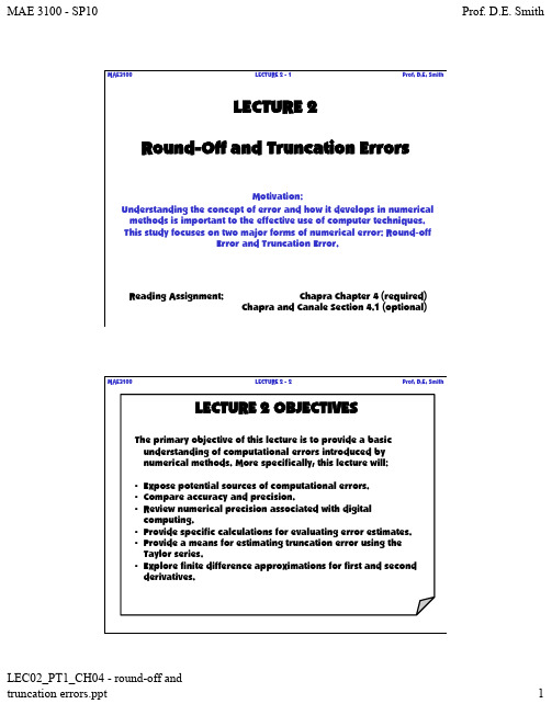
LECTURE 2 -1MAE3100Prof. D.E. SmithLECTURE 2Round-Off and Truncation ErrorsMotivation:Understanding the concept of error and how it develops in numerical methods is important to the effective use of computer techniques.This study focuses on two major forms of numerical error: Round-offError and Truncation Error.Reading Assignment:Chapra Chapter 4 (required)Chapra and Canale Section 4.1 (optional)LECTURE 2 -2MAE3100Prof. D.E. SmithLECTURE 2 OBJECTIVESThe primary objective of this lecture is to provide a basicunderstanding of computational errors introduced bynumerical methods. More specifically, this lecture will:•Expose potential sources of computational errors.•Compare accuracy and precision.•Review numerical precision associated with digitalcomputing.•Provide specific calculations for evaluating error estimates.•Provide a means for estimating truncation error using theTaylor series.•Explore finite difference approximations for first and secondderivatives.MAE3100Prof. D.E. SmithLECTURE 2 -3You’ve Got A Problem•The numerical methods solution to the bungee jumper problem inChapter 1 employed an approximation to the derivative as•What is known?–Numerical error is introduced byapproximation–Approximation error depends on t–Computers have limited precision•What is needed?– A basic understanding of errors associated with computercalculations– A method for assessing the amount of error introduced withthe approximations used by numerical methodsii i i t t t v t v t v dt dv 11)()(MAE3100Prof. D.E. SmithLECTURE 2 -4Sources of Error•Errors in mathematical modelingResult from simplifying assumptions and approximations madewhen representing physical systems by mathematical equations.•BlundersResult from mathematical modeling errors and/or programmingerrors.•Errors in inputBEWARE: garbage in –garbage out•Machine errorsResult from rounding, chopping, underflow and overflow•Truncation errorsResult from simplifying assumptions and approximations madein the numerical procedureOccurs when truncating an infinite series or numericalevaluation of an improper integral. E.g.,!4!3!21432x x x x e xMAE3100Prof. D.E. SmithLECTURE 2 -5Accuracy and Precisiondata scatterdefinesimprecisionoruncertaintysystematic deviation defines inaccuracy or bias inaccurateandimpreciseaccurateandprecise MAE3100Prof. D.E. SmithLECTURE 2 -6Significant Figures•The significant digits of a number are those that can be used withconfidence.•What is the speed?–48 or 49?–48.8 or 48.9?–48.8642138?–#sig-figs = 3•What is the mileage?–87324.4 or 87324.5?–87324.46?–#sig-figs = 7•All results in MAE3100 must display appropriate units and Sig-Figs–Use no less than 3 sig-figs, 4 is preferred–Use the greatest accuracy possible during calculations–Report result with sig-figs consistent with inputMAE3100Prof. D.E. SmithLECTURE 2 -7Error Definitions•True (Absolute) ErrorNote: Issues arise when working with different orders-of-magnitude•True Percent Relative Error•Approximate Percent Relative Error (true value not always known)• A specified percent tolerance s may be used as a stopping criteria:I.e., stop with n decimal place accuracy when ionapproximat value true t E (100%) value true ionapproximat - value true (100%) value true error true t %)100(ion approximat current ionapproximat previous -ion approximat current (100%)ion approximat errore approximat a )%105.0(2n s a MAE3100Prof. D.E. SmithLECTURE 2 -8Round-Off Error•Recall that numbers are stored in binary format–16 bit integer representationRange: -32,768 to 32,767Shown: -173–Floating point representation•Single precision (32 bit)24 bit mantissa7-8 sig-figs Range: 10-38to 1039•Double precision (64 bit)15-16 sig-figsRange: 10-308to 10308Representation used by MATLAB (223210)272625242330292831….sMAE3100Prof. D.E. SmithLECTURE 2 -9Working with Computer Numbers•Computers work in base 2 making it impossible to accuratelyrepresent numbers of interest, e.g.,•MATLAB commands related to machine precision include realmax ,realmin , eps•Round-off errors can accumulate in large computations.•Loss of significant figures occurs when subtracting numbers ofsimilar magnitude:•Small numbers can be lost when added to large numbers using finitemachine precision 333100001.0107641.0107642.0...,7,,,1.0etc e 4444104000.010*******.010*******.0104000.0chopped MAE3100Prof. D.E. SmithLECTURE 2 -10Truncation Error•Taylor theorem : Any smooth function can be written as a polynomial.•Definition: The Taylor Series expansion of f (x )about x = a iswhere the remainder is•The n -th order Taylor Series with h = x –a becomes:• A Maclaurin Series is a Taylor Series expanded about a = 0 (h = x )nk nk k R a x a f k x f 0)()()(!1)(n -th order Taylor Series approximation f n (x )remainder))(()()()!1(111)1(n n n n a x O a x f n R x a nn n hn a f h a f h a f h a f a f h f !)(!3)(!2)()()()()(3)3(2 nn n xn f x f x f x f f x f !)0(!3)0(!2)0()0()0()()(3)3(2 error is ‘on the order of’(x -a )n +1a x XI (ks-eye)MAE3100Prof. D.E. SmithLECTURE 2 -11Truncation Error (cont.)•Accuracy increases as more terms are added to the Taylor Series expansionconstant)a (i.e., 0a function)linear a (i.e., 10h a a )polynomial order 2nd a (i.e.,2210h a h a a MAE3100Prof. D.E. SmithLECTURE 2 -12Taylor Series ExampleFrom Chapra Figure 4.2, pg. 68:Where) (i.e., 0about Expanded 2.125.05.015.01.0)(234x a x h a x x x x x f 0.1)0(25.0)0(2.1)0(f f f xx f 25.02.1)(1225.025.02.1)(x x x f 2.1)(0x fMAE3100Prof. D.E. SmithLECTURE 2 -13Taylor Series -ExampleDetermine the 4-th order Taylor Series of y (x ) = ln(1+x )about x = a = 0By successive differentiation we obtainThe Taylor Series for |x |≤ 1becomes:Note: The error is proportional to x 5: i.e., when x is reduced by afactor of 2, R 4decreases by a factor of 25= 32)1ln()(x x y 0)0(y x x y 11)(1)0(y 2)1(1)(x x y 1)0(y 3)3()1(2)(x x y 2)0()3(y 4)4()1(6)(x x y 6)0()4(y 4324413121)()(x x x x x y x y )()1(51120)(5555)5(4x O x x y R with 5)5()1(24)(y MAE3100Prof. D.E. SmithLECTURE 2 -14Defining the RemainderRecall that the remainder R n is defined in terms the variable asConsider a zero-order (n = 0)Taylor Seriesthen 1)1()()!1()(n n n a x n f R ha a where )()()(0a f x f x f hR f h f R 00)()(= a = x = a = x)(f xa a+hMAE3100Prof. D.E. SmithLECTURE 2 -15Defining the Remainder (cont)Recall our example y (x ) = ln(1+x )with the 4-th order Taylor Series aboutx = 0The remainder becomesCombining these equations givesFor x = 1, we obtainthen or which satisfies the condition 4432413121)(R x x x x x y 55432)1(151413121)1ln(x x x x x x 555554)1(151)0())1(ln(!51x x x dx d R x 12739.058333.0413121)(69315.0)(4324x x x x x y x y 105544)1()1(15110981.058333.069315.0)1()1(y y R MAE3100Prof. D.E. SmithLECTURE 2 -16Defining the Remainder (cont)NOTE:•Determining the number of terms required for a Taylor series torepresent a function of interest is based on the remainder.•Unfortunately, ξis not known exactly but merely lies somewherebetween a and x = a + h (or x i and x i+1).•Also, R n requires derivatives of f (x ),which are not generally known.•Despite this, R n is still useful for gaining insight into truncationerrors.•Recall that we do have control over h and can therefore assess whathappens as we change h , i.e.,1)1(1)1()!1()()()!1()(n n nn n h n f a x n f R )())((11n n n h O a x O R xa a+h hMAE3100Prof. D.E. SmithLECTURE 2 -17Using the Remainder R n1)Establish order of error (from definition)2)Verify order of error estimate*> at h = 0.5 > at h = 1.03) Provide error estimate when h is increased or reduced*at h = 0.5, we computed R 4= 0.00442344then at h = 1.0 (doubled), we estimate R 4(0.00442344)(25) = 0.141550))(()()!1()(11)1(n n n n a x O a x n f R 0.109814)1()1(44y y R 0.00442344)5.0()5.0(44y y R 2X ~25X note: 25= 32X*For y (x ) = ln(1+x )about x = 0MAE3100Prof. D.E. SmithLECTURE 2 -18Using the Remainder R n (cont)4)Calculate value of ξwhen exact function value is known*Recall for h = 1and 5)Establish upper or lower bound on error*Recall that when h = 1, we obtain and Then the upper bound of the error may becalculated as the maximum R 4over the validrange of ξas 0.109814)1()1(44y y R *For y (x ) = ln(1+x )about x = 0554)1()1(151R Equating andsolving for ξgives12739.01054)1(151R 51)1(151)1(15110max 055max 4R maxξR 4MAE3100Prof. D.E. SmithLECTURE 2 -19Numerical DifferentiationDerivatives may be evaluated numerically withthe Finite (Divided) Difference method.1.Forward Difference (error is O (h ))2.Backward Difference (error is O (h ))3.Central Difference (error is O (h 2))hx f h x f x f )()()(hh x f x f x f )()()(hh x f h x f x f 2)()()(MAE3100Prof. D.E. SmithLECTURE 2 -20Remainder w/ Finite DifferenceConsider the 1st order Taylor Series and Remainder for f (x )expandedabout a = x (note h = x )which can be rearranged to give forward differenceExample problem: consider f (x ) = sin(x ) at x = /4exact derivative:forward finite difference:error bounded by remainder:2!2)()()()(xf x x f x f x x f R 1xf x x f x x f x f 2)()()()(O (x )7071067811.0)cos()(4/x x x f 6706029729.01.0)4/sin()1.04/sin()(x f (with x = 0.1)error = 0.0370781.04/at 0.0387084/at 0.035355)(2)sin(2)(x x f。
Lecture 10_Index Number 第十章 指数

Special purpose Combines and weights a Value heterogeneous group of series Measures the change in the to arrive at an overall index value of one or more items showing the change in from the base period to the business activity from the given period (PxQ). base period to the present.
Lecture 5
Index Number
Lecture 5_Index Numbers
GOALS When you have completed this chapter, you will be able to:
ONE Describe the term index. TWO Understand the difference between a weighted price index and an unweighted price index. THREE Construct and interpret a Laspeyres Price index. FOUR Construct and interpret a Paasche Price index.
where pt is the current price p0 is the price in the base period q0 is the quantity consumed in the base period
Paasche Weighted Price Index, P
Lecture_10_stresses_and_strains_3

1 CIV 2016A Soil MechanicsLecture 10: Stresses, Strains And Elastic Deformation of Soils 3Book Chapter: 7Section: 7.11 –7.12 Pages: 162 To 181Stresses in Soils from Surface Loads Book Chapter: 7Section: 7.11 –7.12 Pages: 162 To 181Learning outcomes3☐Know the assumptions made in estimating ∆σz on a soil from surface loads.☐Be able to calculate ∆σz from common types ofsurface loads.Vertical Stress at A Point in Soil4σz = Vertical overburden stress (geostatic stress, in-situ stress) induced by weight of soil∆σz = Additional stress induced by external loadsImportance5☐The stresses we have considered so far are calledgeostatic stresses.☐In practice, loads are applied either on the groundsurface or within the soil mass. At any given depthz, we have to be able to calculate ∆σz on the soilfrom these applied loads to determine if the soil has the strength and stiffness to support the appliedloads.Some Common Types of Surface Loads☐Types of surface loadsFinite and infinite -qualitativeclasses and are subject tointerpretation.☐Examples of finite loadspoint loads (electric powerpole)circular loads (foundation fora tank)rectangular loads (foundationfor a column)☐Examples of infinite loadsFills (embankment for a road) Surcharges6Estimation of ∆σz in Soils from Surface Loads☐Joseph Valentin Boussinesq(1885) presented a solution for thedistribution of stresses for a pointload applied on the soil surface☐AssumptionsSoil is a semi-infinite, homogeneous, linear,isotropic, elastic material. ❑ A semi-infinite mass is bounded on one side and extends infinitely in all otherdirections; this is also called an “elastic half-space.” For soils, the horizontalsurface is the bounding side.❑Because of the assumption of a linear elastic soil mass, we can use theprinciple of superposition.❑That is, the stress increases at a given point in a soil mass from differentsurface loads can be added together.7Stress Increase due to Surface Loads8Boussinesq Solution2z Q I z σ∆=Illustration L >> BApproximate methodVariation of ∆σz with Depth and Lateral Distance from the Loaded Area?☐∆σz decreases with depth ☐At about a depth of 2B , ∆σz ≤ 10% q s12∆σzD e p t h2B≈0.1q s☐∆σz decreases away (laterally) fromthe loaded area.∆σzLateral distance from loaded areaQ is the applied surface load, z is depth, I is the influence factor00.10.20.30.40.50.600.511.522.5Ir/z2z Q I zσ∆=Q is the applied surface load per unit length, z is depth, I is the influence factor2z Q Izσ∆=00.050.10.150.20.250.30.3500.511.522.53Ix/zStress Chart for A Strip Loadq s is the applied surface stress, I is the influence factor (the value on each isobar)15z s q Iσ∆=Vertical Stress Induced by Strip Loading16Check p166, sec 7.11.4of Budhu’s book☐q s is the applied surface stress☐I c is the influence factor (the value on each isobar)()3/220111/ z s s cq r z q I σ∆=−+=q s is the applied surfacestress, I z is the influence factor (the value on each isobar)z s zq I σ∆=The number on the isobar is I z19Vertical Stress Induced by A Rectangularly Loaded Arearadian, if <0, then add πn=z/LStress Chart for A Rectangular Load☐q s is the applied surfacestress, I z is the influence factor (the value on each isobar)☐Stress increase is valid for a corner of the rectangle .20z s zq I σ∆=Stress Distribution Method (2:1 Method)21()()2tan 2tan z s sLB LBq q L B L z B z σαα==′′++If tan α= 1/2()()z s LBq L z B z σ∆=++2:1 MethodStress Chart for An Embankment Load☐q s = γH is the applied surface stress, H is the height of the embankment☐I is the influence factor☐Stress increase is valid for one half width of embankment. Multiply the results by 2 for the full embankment.22z s q Iσ∆=The number on the isobar is I zStress Chart for An Irregular Load☐Newmark (1942) developed a chart to determine ∆σz due to a uniformly loadedarea of any shape .☐The chart consists of concentric circles divided by radial lines☐The area of each segment represents an equal proportion of the applied surface stress at a depth z below the surface.☐The chart is normalized to the depth z ; that is, all dimensions are scaled by a factor initially determined for the depth.☐Every chart should show a scale and aninfluence factor I N . The influence factor for the chart shown is 0.001.23Procedure to Use the Stress Chart for An Irregular Load☐Set the scale equal to the depth at which ∆σz is required. We call it the depth scale☐Identify the point A below the loaded area where the stress is required. ☐Plot the loaded area, scaling its plan dimension using the depth scale with point A at the center of the chart.☐Count the number of segments (N s ) covered by the scaled loaded area. fraction is allowed.☐Then 24z s N sq I N σ∆=AVertical Stress Below Arbitrarily Shaped Areas252000.0056161 kPaz s N sq I N σ∆=××200 kPas q ==−[]1234zs z z z z q I I I I σ∆=+++[]1234zs z z z z q I I I I σ∆=+−−=−[]1234zs z zz z q I I II σ∆=−−+−+Application 28Key Points☐The ∆σz below a surface load are found by assuming the soil is an elastic, semi-infinite mass.☐Various equations are available for ∆σz from surface loading.☐∆σz at any depth depends on the shape and distribution of the surface load.☐ A stress applied at the surface of a soil mass by a loaded area decreases with depth and lateral distance away from the center of the loaded area.☐∆σz<0.1q s when z/B ≥ 2.2930 On Your Own:1. Read The Material Covered In This Lecture From The Textbook.Next Lecture:Book Chapter: 8Section: 8.0 –8.5 Pages: 186 To 203。
Approximate Computing - ETS Tutorial 2013 2PerPage

Stochastic logic models: (a) An unreliable AND gate; (b) A general stochastic implementation; (c) for soft errors; (d) for stuck-at-1 fault; (e) for stuck-at-0 fault [Han14]. © 2013 Han and Orshansky
2014/6/25
Approximate Computing: An Emerging Paradigm For Energy-Efficient Design
Jie Han and Michael Orshansky
University of Alberta and University of Texas at Austin Embedded Tutorial, ETS’13, Avignon, France
A tradeoff between switching probability and associated energy: energyprobability relationship of an XOR gate [Palem12]
Embedded Tutorial, ETS’13, Avignon, France
approximate computing applications
Embedded Tutorial, ETS’13, Avignon, France
© 2013 Han and Orshansky
Outline
MOTIVATION OVERVIEW OF ERROR-RESILIENT PARADIGMS APPROXIMATE ARITHMETIC CIRCUITS Approximate adders Approximate multipliers Metrics for approximate computing Quality-energy optimal designs Approximate logic synthesis ALGORITHM-LEVEL APPROXIMATE COMPUTING
移动互联网导论(第3版)课件10_WiMax

Estimated attenuation due to rain:
A aRb
A = attenuation (dB/km) R = rain rate (mm/hr) a and b depend on drop sizes and frequency
Increasing interest shown in competing wireless technologies for subscriber access Wireless local loop (WLL)
– Narrowband – offers a replacement for existing telephony services
– Peak of water vapor absorption at 22 GHz – Peak of oxygen absorption near 60 GHz
Favorable windows for communication:
– From 28 GHz to 42 GHz – From 75 GHz to 95 GHz
– With a wired system, cable is laid out in anticipation of serving every subscriber in a given area
Electronic Engineering
Dr. Xinbing Wang
5
Propagation Considerations for WLL
– Encoding/decoding of signals – Preamble generation/removal – Bit transmission/reception
Methodologies] Symbolic and Algebraic Manipulation —Algorithms G.1.2 [Mathematics of Compu
![Methodologies] Symbolic and Algebraic Manipulation —Algorithms G.1.2 [Mathematics of Compu](https://img.taocdn.com/s3/m/7fba8e155f0e7cd1842536ab.png)
Hybrid Symbolic-Numeric Computation*Erich KaltofenDepartment of MathematicsMassachusetts Institute of T echnology Cambridge,Massachusetts02139-4307,USA kaltofen@Lihong ZhiKey Laboratory of Mathematics Mechanization Academy of Mathematics and Systems ScienceBeijing100080,Chinalzhi@/~lzhiCategories and Subject Descriptors:I.2.1[Comput-ing Methodologies]:Symbolic and Algebraic Manipulation —Algorithms;G.1.2[Mathematics of Computing]:Numeri-cal Analysis—ApproximationGeneral Terms:algorithms,experimentation Keywords:symbolic/numeric hybrid methodsTUTORIAL ABSTRACTSeveral standard problems in symbolic computation,such as greatest common divisor and factorization of polynomials, sparse interpolation,or computing solutions to overdeter-mined systems of polynomial equations have non-trivial so-lutions only if the input coefficients satisfy certain algebraic constraints.Errors in the coefficients due tofloating point round-offor through phsical measurement thus render the exact symbolic algorithms unusable.By symbolic-numeric methods one computes minimal deformations of the coeffi-cients that yield non-trivial results.We will present hybrid algorithms and benchmark computations based on Gauss-Newton optimization,singular value decomposition(SVD) and structure-preserving total least squares(STLS)fitting for several of the above problems.A significant body of results to solve those“approximate computer algebra”problems has been discovered in the past 10years.In the Computer Algebra Handbook the section on “Hybrid Methods”concludes as follows[2]:“The challenge of hybrid symbolic-numeric algorithms is to explore the ef-fects of imprecision,discontinuity,and algorithmic complex-ity by applying mathematical optimization,perturbation theory,and inexact arithmetic and other tools in order to solve mathematical problems that today are not solvable by numerical or symbolic methods alone.”The focus of our tu-torial is on how to formulate several approximate symbolic computation problems as numerical problems in linear al-gebra and optimization and on software that realizes their solutions.∗This research was supported in part by the National Science Foun-dation of the USA under Grants CCR-0305314and CCF-0514585 (Kaltofen)and OISE-0456285(Kaltofen,Yang and Zhi).This research was partially supported by NKBRPC(2004CB318000) and the Chinese National Natural Science Foundation under Grant 10401035(Yang and Zhi).Kaltofen’s permanent address:Dept.of Mathematics,North Car-olina State University,Raleigh,North Carolina27695-8205,USA, kaltofen@.Copyright is held by the author/owner(s).ISSAC’06,July9–12,2006,Genova,Italy.ACM1-59593-276-3/06/0007.Approximate Greatest Common Divisors[3].Our pa-per at this conference presents a solution to the approximate GCD problem for several multivariate polynomials with real or complex coefficients.In addition,the coefficients of the minimally deformed input coefficients can be linearly con-strained.In our tutorial we will give a precise definition of the approximate polynomial GCD problem and we will present techniques based on parametric optimization(slow) and STLS or Gauss/Newton iteration(fast)for its numeri-cal solution.The fast methods can compute globally optimal solutions,but they cannot verify global optimality.We show how to apply the constrained approximate GCD problem to computing the nearest singular polynomial with a root of multiplicity at least k≥2.Approximate Factorization of Multivariate Polyno-mials[1].Our solution and implementation of the approx-imate factorization problem follows our approach for the approximate GCD problem.Our algorithms are based ona generalization of the differential forms introduced by W.Ruppert and S.Gao to many variables,and use SVD or STLS and Gauss/Newton optimization to numerically com-pute the approximate multivariate factors.Solutions of Zero-dimensional Polynomial Systems[4].We translate a system of polynomials into a systemof linear partial differential equations(PDEs)with constant coefficients.The PDEs are brought to an involutive form by symbolic prolongations and numeric projections via SVD.The solutions of the polynomial system are obtained by solv-ing an eigen-problem constructed from the null spaces of the involutive system and its geometric projections.1.REFERENCES[1]Gao,S.,Kaltofen,E.,May,J.P.,Yang,Z.,andZhi,L.Approximate factorization of multivariatepolynomials via differential equations.In Gutierrez,J.,Ed.ISSAC2004Proc.2004Internat.Symp.Symbolic Algebraic Comput.,pp.167–174.[2]Grabmeier,J.,Kaltofen,E.,and Weispfenning,puter Algebra Handbook Springer Verlag,2003,pp.109–124.[3]Kaltofen,E.,Yang,Z.,and Zhi,L.Approximategreatest common divisors of several polynomials withlinearly constrained coefficients and singularpolynomials.In Dumas,J-G.,Ed.ISSAC2006Proc.2006Internat.Symp.Symbolic Algebraic Comput..[4]Reid,G.,Tang,J.,and Zhi,L.A completesymbolic-numeric linear method for camera posedetermination.In Sendra,J.,Ed.ISSAC2003Proc.2003Internat.Symp.Symbolic Algebraic Comput.,pp.215–223.7。
形近近义词总结

第一节同源异义词1.alike a. 同样的,相像的(常作表语)like a. 相像的,相同的(常作定语)prep. 像…;v. 喜欢(~ to do / ~ doing)likely a. ad. 可能的/地(be ~ to do /be ~ that)unlike prep. 不像…(那样)dislike v. 不喜欢[例]The twins don’t look alike.They are very likely to win the game.Unlike his father, he doesn’t like painting. 2.alive a. 活的,活生生的(作表语或补语)live a. 活的(作定语,修饰有生命的动物)现场直播的(a live broadcast)living a. 活着的,现存的(~ language)逼真的;强烈的,活泼的(a ~ hope)lively a. 活泼有生气的,快活的;鲜明的[例]He was still alive though badly injured.He is doing an experiment with live mice.He is the greatest living actor.3.alone a. 孤单的(只作表语)ad. 单独地lonely a. 孤单的,寂寞的(强调孤单的感觉)[例]I’m alone but not lonely.It was Tom who finished the job alone.4.considerable a. 大量的,同a lot ofconsiderate a. 体贴的,为他人着想的considered a. 慎重的,经过细致考虑的[例]Writing needs considerable reading andthinking.It is considerate of you to close the door.I’ll never change my mind once I made aconsidered decision.5.exhaustible a. 会耗尽的,可用完的exhausting a. 使耗尽的,令人筋疲力尽的exhaustive a. 消耗的;全面彻底的,完全的exhausted a. 筋疲力尽的[例]Coal is a type of exhaustible resource.This is an exhausting task.I was exhausted after the long journey.An exhaustive analysis of the policy6.imaginary a. 想像的,虚构的imaginative a. 有想像力的imaginable a. 可想像得到的[例]The story is imaginary, not real.The imaginative boy made up the story.We met the greatest difficulty imaginable.7.respective a. 各自的,分别的respectful a. 恭敬的,充满敬意的respectable a. 可敬的,正派的[例]Mr. Li is a respectable professor.Linda is respectful towards her teacher.After the lecture, the respectable profess-or and the respectful students went backto their r espective rooms.8.social a. 社会的;交际的,社交的sociable a. 好交际的,友好的,合群的[例]This novel is of great social significance.He’s a sociable person.9.sensitive a. 敏感的,过敏的(be ~ to sth.)sensible a. 明智的,知道的;可感知的[例]The eyes are sensitive to light.He is sensible of the danger of his position.10.economic a. 经济上的,有利可图的economical a. 节约的,节省的( be ~ of sth.) [例]Their economic prospects are grim.One must be economical of one’s time. 11.distinct a. 有区别的,清晰的,明确的distinctive a. 表示有别的,有特色的[例]The earth’s shadow on it is quite distinct.Soldiers wear a distinctive uniform.12.decided a. 决定了的;明显的,明白无误的decisive a. 决定性的;明确的;坚定果断的[例]I am quite decided about it.Mr. Li’s opinion is decisive on this matter.13.confident a. 有信心的,自信的confidential a. 机密的,秘密的confidant n. 知己,密友confidence n. 信心,信赖[例]We were confident of the victory.He is confident in the future.parable a. (to/with) 可与相比,可比较的comparative a. 相对的,比较而言的[例]The sets of figures are not comparable.This house is comparatively cheap.fortable a.(使人)舒服的,轻松的comforting a. 安慰的,令人欣慰的[例]—a comfortable chair 舒适的椅子—comforting words 安慰的话16.satisfied a. 满意的,满足的(be ~ with)satisfying a. 令人满意的satisfactory a. 令人满意的,可喜的[例]I was satisfied with his reply.His reply is not satisfying / satisfactory. 17.continuous a. 连续不断的(动作没有间歇)continual a. 连续的(可有短暂间歇)[例]the continuous ticking of clock.I hate the continual quarrels with my wife.18.practical a. 实际的,实用的practicable a. 可实行的,可做的[例]—to overcome the practical difficulties—methods that are not practicable19.industrious a. 勤勉的,刻苦的industrial a. 工业的,产业的[例]He is a very industrious student.—The Industrial Revolution20.visible a. 可见的,能看见的visual a. 看的,视觉的[例]The eclipse will be visible to all observers.Visual organ is a medical term for “eye”. 21. personal a. 个人的,人身的,亲身的personnel n. 职员,(尤指公职或军职)人员[例]These are all my personal belongings.There are 5 personnel on that plane.22 regrettable a. 令人遗憾的,可惜的regretfu l a. 抱歉的,遗憾的,哀惜的[例]It is regrettable that he behaved like that.I felt regretful about what happened.第二节非同源形近词1.adapt v. 使适应;改编adopt v. 采用;收养[例]He adapted himself quickly to the new life.This film is adapted from a novel of Luxun.The old couple adopted another boy.This technique has been widely adopted. 2.angel n. 天使angle n. 角度,观点[例]What angle are you writing the story from?3.familiar a. 熟悉的(be ~ to / with)similar a. 相似的(be ~ to )[例]We are familiar with this kind of situation.These words are familiar to us.This novel is similar to that one.4.contact n. 接触,联系vt. 与…接触in ~ withcontract n. 契约,合同v. 订合同;收缩[例]We finally made contact with him in Paris.We entered into a contract with that firm.5.desert n. 沙漠v. 抛弃dessert n.(餐后)甜食[例]Don’t desert your friend in their misfortune.Does the price of the meal include dessert?6.vocation n. 职业,天职,能力vocational a.vacation n. 假日,假期be on ~ 在度假[例]I mistook my vocation. 我选错了职业。
有限差分法讲义

(
)
P (x, t) = (γ − 1) E − 1 ρu2 ,
2
and γ is the ratio of the specific heats (assumed constant).
Example 1.6 (The Shallow Water Equations)
For a liquid with waves large compared to the liquid’s depth, the velocity u(x, t) and liquid
Example 1.1 (The Heat Equation)
For as solid material of constant thermal diffusivity κ in three dimensions x, y, z, the evolu-
tion (in time t) of the temperature T (x, y, z, t) within the material is governed by the Heat
∂E ∂E + E = 0.
∂t ∂x More complicated PDEs arise when modelling situations with many dependent variables.
Example 1.5 (Inviscid Compressible Flow in 1-D: Euler’s Equations)
∇2(ϕ)
=
div(grad(ϕ))
=
∇
·
∇(ϕ)
=
∂2ϕ ∂x2
+
∂2ϕ ∂y2
+
∂2ϕ ,
∂z2
- 1、下载文档前请自行甄别文档内容的完整性,平台不提供额外的编辑、内容补充、找答案等附加服务。
- 2、"仅部分预览"的文档,不可在线预览部分如存在完整性等问题,可反馈申请退款(可完整预览的文档不适用该条件!)。
- 3、如文档侵犯您的权益,请联系客服反馈,我们会尽快为您处理(人工客服工作时间:9:00-18:30)。
The stiffness characteristics are represented by obtaining a stiffness matrix for each element based on an assumed deflection shape within the element. The mass characteristics are either lumped at each node or a consistent element mass matrix
∆M&& + v = ∆fv (t) v
∆ = K−1
(ii) Finite Element method-The structure is divided into methodelements with the deflection of the structure represented by the deflection/rotation of nodal points (at the extremum/center of each element).
produced (equivalent) in kinetic energy terms to the behaviour of the element when it deflects as assumed). The element mass and stiffness matrices are then assembled to yield equations of the form,
Or
v1 δ11 δ12 F 1 = v2 δ21 δ22 F2 v = ∆F
where ∆ is the flexibility matrix for points 1 and 2.
−1 Now F = ∆ v = Kv , so the stiffness matrix is K = ∆−1 . However it is not necessary to invert the flexibility matrix to obtain equations of motion when the two masses are added. Instead if F1 and F2 are the forces applied to the beam by the masses at some instant of time then there are equal and opposite forces applied to the masses by the beam.
Lecture 10 Introduction to Vibration of Continuous SystemsSystems-3 Approximate Methods
There are two basic approaches: a) Assumed shapes (Rayleigh Ritz) b) Discretisation -Flexibility influence coefficients -Finite Elements
represented by the deflection/rotation of the center of each section.
The stiffness characteristics are represented using flexibility influence coefficients which yield a flexibility matrix for the entire structure. The mass characteristics are concentrated at the center of each section (mass, moment of mass and moment of inertia). Equations are of the form,
The resulting deflections define the flexibility influence coefficients, typically
δij is the deflection at i due to a unit force at j. The units
are m/N and the values come from beam theory in Strength of Materials. Maxwell’s reciprocal theorem can be shown to apply for linear systems where superposition can be applied, i.e.
Flexibility Influence Coefficients
aij Lateral deflection at point i due to unit lateral load at point j. a ji Lateral deflection at point j due to unit lateral load at point i Note: 1. aij = a ji by Maxwell’s Reciprocal Theorem. 2. “Long” and “Short” bearings are essentially equivalent to clamped and simple supports respectively.
&& & Mq + Cq + Kq = f
The equations may be solved using standard multi-DOF multimethods. Note that the amplitude ratios and hence mode shapes will be expressed as a combinat ij= δ ji
The principle of superposition may then be used to find the deflections v1 and v2 due to F1 and F2 acting simultaneously, namely
v1 = δ11F +δ12F2 1 v2 = δ21F +δ22F2 1
Now, treat the structure as a beam under the action of forces in order to find its flexibility characteristics (flexibility=1/stiffness) Consider a unit force at position 1, and then position 2, 2,
B. DISCRETISED
Here there are two basic method: (i) Flexibility Influence Coefficients-The structure is Coefficientsdivided into sections/lumps with the deflection of the structure
v(x, t) = φ1(x)q1(t) +φ2 (x)q2 (t) +L v(x, t) = Φ(x)T q(t)
The equations of motion may be set up in terms of the generalized coordinates using Lagrange, PVD or Principle of Minimum Total Potential Energy and will be in the form,
M&& + Kv = fv (t) v
In each method, the generalized coordinates are the displacement/rotation of selected points based on spatial discretisation. The equations may be solved using standard multi-dof methods. multi-
Flexibility Influence Coefficients
Continuous systems are often idealized into “lumps” or
sections, connected by massless springs. In order to represent the stiffness behaviour, it is sometimes convenient to use the idea of “flexibility influence coefficients”. Consider the example of a beam-structure beam(may be applied equally as well to a plate etc) and if “rocking” of each lump is ignored, there are 2 dof.
A. ASSUMED SHAPES
Here the deflection of the structure is represented approximately by a series of known deflection shapes multiplied by unknown (generalized) coordinates. For example, in a beam-like structure, beam-
Or
&& δ11m δ12m2 v1 1 0v1 0 1 δ m δ m v + 0 1v = 0 2 21 1 22 2 &&2