Solving Nonlinear Equation Systems Using Evolutionary Algorithms ABSTRACT
朗道十卷英文名
朗道十卷英文名朗道十卷是世界著名物理学教材。
朗道十卷英文名如下所示。
一、《朗道理论物理学教程第一卷:力学》Course of Theoretical Physics Volume one: Mechanics二、《朗道理论物理学教程第二卷:场论》Course of Theoretical Physics Volume two: The Theory of Fields三、《朗道理论物理学教程第三卷:量子力学(非相对论理论) 》Course of Theoretical Physics Volume three: Quantum Mechanics (Non-relativistic Theory)四、《朗道理论物理学教程第四卷:量子电动力学》Course of Theoretical Physics Volume four: Quantum Electrodynamics 五、《朗道理论物理学教程第五卷:统计物理学》Course of Theoretical Physics Volume five: Statistical Physics六、《朗道理论物理学教程第六卷:流体动力学》Course of Theoretical Physics Volume six: Fluid Mechanics七、《朗道理论物理学教程第七卷:弹性理论》Course of Theoretical Physics Volume seven: Theory of Elasticity八、《朗道理论物理学教程第八卷:连续介质电动力学》Course of Theoretical Physics Volume eight: Electrodynamics of Continuous Media九、《朗道理论物理学教程第九卷:统计物理学》Course of Theoretical Physics Volume nine: Statistical Physics十、《朗道理论物理学教程第十卷:物理动理学》Course of Theoretical Physics Volume ten: Physical Kinetics。
evolution equations
Abstract
1 Introduction
The KdV 2-soliton solution regarded as the interaction of two single solitons has been investigated by several authors 1] - 5]. In 1] - 3] the decomposition of the 2-soliton solution was achieved via inverse scattering transform theory. In 4, 5], however, the Hirota formalism was used. The results in 3] and 4, 5] were later extended to the KdV N -soliton solution; see 6] and 7] respectively. The decomposition in 6] and 7] is, in fact, applicable to a wide class of nonlinear evolution equations of which the KdV equation is a member, and it is this class of equations that is considered here. In x2 we summarise the formulation of the decomposition of the N -soliton solution. In x3 we focus on the case N = 2. In x4 and x5 we illustrate our results by considering an extended KdV equation and the Sawada-Kotera equation respectively. Future work is outlined in x6.
涉及非体积功的热力学基本方程
第49卷第8期2021年4月广州化工Guangzhou Chemical IndustryVol.49No.8Apr.2021涉及非体积功的热力学基本方程杨嫣,陈山川,谢娟,张改(西安工业大学材料与化工学院,陕西西安710021)摘要:热力学基本方程是物理化学课程中一个重要的知识点。
现行物理化学教材中重点阐述了仅含有体积功的热力学基本方程,而对涉及非体积功的热力学基本方程介绍很少。
对材料类专业的学生来说,学习和研究材料热力学,经常会涉及到非体积功。
因此,学习涉及非体积功的热力学基本方程非常必要。
本文重点讨论了涉及非体积功的表面系统、弹性杆、电、磁介质中的热力学基本方程的推导和应用,并总结了处理这类问题的方法。
关键词:物理化学;热力学;基本方程;非体积功中图分类号:G642文献标志码:A文章编号:1001-9677(2021)08-0139-04 Fundamental Equations in Thermodynamics Involving Non-expansion Work*YANG Yan,CHEN Shan-chuan,XIE Juan,ZHANG Gai(School of Material Science and Chemical Engineering,Xi9an Technological University,Shaanxi Xi'an710021,China) Abstract:Fundamental equation in thermodynamics is one of the key points of Physical Chemistry course・In current Physical Chemistry textbooks,the fundamental equations containing only expansionwork are mainly described, while the ones involving non-expansionwork are rarely introduced.For the students majoring in materials,non-expansionwork is often involved in the processes of studyand research.Therefore,it is necessary to study the fundamental equations in involving non-expansion work.The derivations and applications of the fundamental equations in surface systems,elastic rods,electric and magnetic media were discussed.Moreover,the way to deal with this kind of problem was summarized.Key words:Physical Chemistry;thermodynamics;the fundamental equation;non-expansion work热力学基本方程在处理平衡态热力学问题时非常有用,是物理化学课程内容的重点之一。
Existence of Infinitely Many Solutions for a Quasilinear Elliptic Problem on Time Scales
arXiv:0705.3674v1 [math.AP] 24 May 2007
Existence of Infinitely Many Solutions for a Quasilinear Elliptic Problem on Time Scales
Moulay Rchid Sidi Ammi sidiammi@mat.ua.pt
2 Preliminary results on time scales
We begin by recalling some basic concepts of time scales. Then, we prove some preliminary results that will be needed in the sequel.
Delfim F. M. Torres delfim@mat.ua.pt
Department of Mathematics
University of Aveiro 3810-193 Aveiro, Portugal
Abstract
We study a boundary-value quasilinear elliptic problem on a generic time scale. Making use of the fixed-point index theory, sufficient conditions are given to obtain existence, multiplicity, and infinite solvability of positive solutions.
《2024年非线性耦合方程组的高阶无振荡有限体积方法》范文

《非线性耦合方程组的高阶无振荡有限体积方法》篇一一、引言在科学与工程领域,非线性耦合方程组的求解是一项关键技术。
其精确性与稳定性对多种问题,如流体动力学、电路模拟和材料科学等具有重要意义。
为了更好地处理这些问题,研究者们提出了一种高阶无振荡有限体积方法。
本文将探讨此方法在非线性耦合方程组中的应用。
二、非线性耦合方程组的基本概念非线性耦合方程组由多个非线性偏微分方程组成,它们在空间和时间上相互依赖和影响。
这种复杂性使得求解过程变得复杂且计算量大。
为了解决这一问题,我们需要寻找一种有效的数值求解方法。
三、高阶无振荡有限体积方法高阶无振荡有限体积方法是一种求解偏微分方程的有效数值方法。
它利用有限体积的概念将求解空间离散化,通过求解离散化后的方程来逼近原方程的解。
此方法具有高精度、无振荡的特性,特别适合于求解非线性耦合方程组。
四、高阶无振荡有限体积方法的实施步骤高阶无振荡有限体积方法的实施步骤主要包括以下几步:1. 空间离散化:将求解空间划分为一系列的有限体积单元,每个单元代表一个离散点或一组离散点。
2. 建立离散化方程:基于高阶导数的空间分布特性,在每个有限体积单元上建立离散化后的偏微分方程。
3. 时间推进:采用合适的时间推进策略(如Runge-Kutta方法)求解离散化后的方程。
4. 迭代与收敛:通过迭代过程逐步逼近原方程的解,同时需要确保解的稳定性和收敛性。
五、高阶无振荡有限体积方法在非线性耦合方程组中的应用将高阶无振荡有限体积方法应用于非线性耦合方程组时,需要考虑以下几点:1. 适当的离散化策略:根据问题的特性选择合适的空间离散化策略,以确保解的准确性和稳定性。
2. 耦合项的处理:对于非线性耦合方程组中的耦合项,需要采用适当的方法进行处理,以保持解的准确性。
3. 时间推进策略的选择:根据问题的特性和需求选择合适的时间推进策略,如显式或隐式时间积分方法等。
六、实验与结果分析我们采用了几种典型的非线性耦合方程组进行实验,并比较了高阶无振荡有限体积方法与其他方法的性能。
参考文献的标准格式1
参考文献著录格式标准规范参考文献应引作者亲自阅过的近年的主要文献,一般文章不超过5篇,评述、综述性文章不超过20篇。
未公开发表的资料请勿引用,但可作脚注处理。
参考文献列于文后,正文中也须用上角标标出引用文献的序号。
参考文献用“顺序编码制”,即各篇文献按其在正文中的标注序号依次列出。
参考文献条目著录:个人著者采用姓在前,名在后的著录格式。
作者3人以下全部著录,4人以上只著录前3人,之间加“,”,后加“等” 或“etal”。
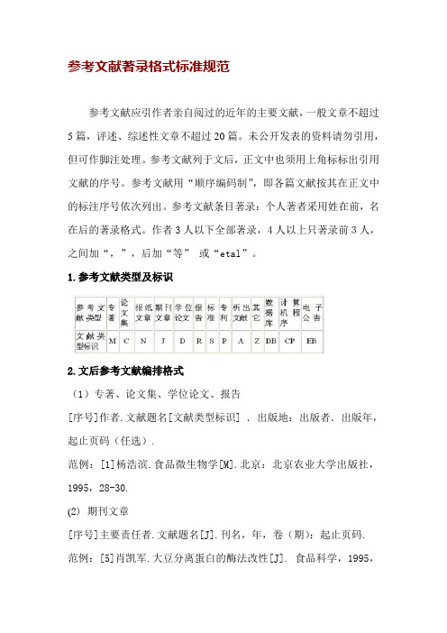
1.参考文献类型及标识2.文后参考文献编排格式(1)专著、论文集、学位论文、报告[序号]作者.文献题名[文献类型标识] .出版地:出版者.出版年,起止页码(任选).范例:[1]杨浩滨.食品微生物学[M].北京:北京农业大学出版社,1995,28-30.(2) 期刊文章[序号]主要责任者.文献题名[J].刊名,年,卷(期):起止页码.范例:[5]肖凯军.大豆分离蛋白的酶法改性[J]. 食品科学,1995,16(9):30-34.范例:[7]OUJP,YOSHIDA O,SOONGT, etal. Recent advance in research on applications energy dissipation systems[J]. Earthquake Eng , 1997,38(3): 358-361.(3) 论文集[序号]作者.文献题名[A].编者.论文题名[C].出版地:出版者,出版年,起止页码.范例:[8]瞿秋白.现代文明的问题与社会主义[A] .罗荣渠.从西化到现代化[C].北京:北京大学出版社,1990,121-133.(4) 报纸文章[序号]作者.文献题名[N].报纸名,出版日期(版次).范例:[10] 胡鞍钢. 中国能够实现粮食自给目标[N].联合早报,1994,10.(5) 国际、国家标准[序号]标准编号,标准名称[S].范例:[11]GB/T 16159-1996 ,汉语拼音正词法基本规则[S]. (6) 专利[序号]专利所有者.专利题名[P].专利国别:专利号,出版日期.范例:[12]姜锡洲. 一种温热外敷药制备方案[P].中国专利:881056073,1989,07,26.(7) 电子文献[序号]作者.电子文献题名[电子文献及载体类型标名].电子文献的出处或可获得地址,发表或更新日期/引用日期(任选).范例:[13]王明亮.关于中国学术期刊标准化数据库系统工程的进展[EB OL]. , 1998,08,16/1998,10,04.(8)各种未定义类型的文献[序号]主要责任者.文献题名.出版地:出版者,出版年.范例:[15]张永禄. 唐代长安词典[Z].西安:陕西人民出版社,1980. 毕业论文参考文献规范格式专著-M;论文集-C;报刊-N;期刊文章-J;学位论文-D;报告-R;专著或论文集中析出的文献-A;标准-S;专利- P;对于不属于上述的文献类型,采用字母“Z”标识。
Non-additive measures and integrals

Non-additive measures and integrals Endre PapDepartment of Mathematics and Informatics,University of Novi SadTrg Dositeja Obradovi´c a4,21000Novi Sad,Serbiae-mail:pape@eunet.yuAbstract:There is presented a short overview on some results related the theory of non-additive measures and the corresponding integrals occurring in several important applications.Key words and phrases:non-additive measure,aggregation function,Choquet integral, Sugeno integral,triangular conorm,triangular norm,pseudo-additive measure.1IntroductionSeveral types of integrals with respect to non-additive measures were devel-oped for different purposes,[1,5,6,15,16].We present some results related the theory of non-additive measures and the corresponding integrals important in several important applications.Many of these applications are related to functions defined onfinite sets and therefore we restrict ourselves here on the finite case.We present also some results on special class of non-additive mea-sures so called pseudo-additive(decomposable)measures and the corresponding integrals,which give a base for the so called pseudo-analysis.There are many important applications,for example in optimization problems,decision making, nonlinear partial differential equations,nonlinear difference equations,optimal control,fuzzy systems,[11,12,15,16].2Non-additive measuresLet us consider I=[0,1]and N={1,...,n}.A set function m on N is a function from2N to R.A subset A⊆N is equivalently denoted by(1A,0A c)∈[0,1]n,or by its characteristic function1A defined over N.We denote x= (x1,...,x n).Using the above equivalence,any set function m bijectively corre-sponds to a pseudo-Boolean function f m:{0,1}n→R by f m(x)=m(A x) for all x∈{0,1}n,where A x={i∈N|x i=1}.Conversely,to any pseudo-Boolean function f corresponds a unique set function m f such thatm f (A ):=f (1A ,0A c ).Pseudo-Boolean functions are widely used in operations research.Cooperative game theory is devoted to a particular class of set func-tions,called transferable utility games in characteristic form .We will call them games or non-additive measure for simplicity.In the context of game theory,the set N is the set of players.A game m :2N →R is a set function satisfying m (∅)=eful examples of games are unanimity games .For any A ⊆N ,the unanimity game u A on N is defined by:u A (B ):= 1,if B ⊇A 0,otherwise.Note that u ∅is not a game since u ∅(∅)=1.A capacity m :2N →R +is a game such that µ(A )≤µ(B )whenever A ⊆B (monotonicity ).A capacity is normalized if µ(N )=1.Capacities are monotonic games,and were introduced originally by Choquet in 1953.They were rediscovered by Sugeno in 1974under the name fuzzy measure [20].Important connection with aggregation functions can be described in the following way,see [6].Suppose we use as an aggregation function the weighted arithmetic mean WAM w (x )=w 1x 1+···+w n x n w −1+···+w nwith respect to some weight vector w ∈[0,1]n .It is easy to relate w to the values taken on by WAM w ,using particular vectors in [0,1]n ,namely 1i :WAM w (1i )=w i for all i ∈N.This means that the value of function WAM w on [0,1]n is solely determined by its value at the endpoints of the n dimen-sions,which represents the weight of each dimension.In fact,the exact way WAM w (x ),x ∈[0,1]n ,is determined from WAM w (1i ),i =1,...,n ,is linear interpolation.One may construct more complicated aggregation functions A by using more points in [0,1]n to determine A .A natural yet simple choice would be to take all vertices of [0,1]n ,namely {1A }A ⊆N .These include the previous endpoints of dimensions.Doing so,we have defined a set of weights {w A }A ⊆N ,byA w (1A )=w A ,A ⊆N.It remains to construct A w on [0,1]n by some means (e.g.,linear interpolation),using these points.By analogy with the previous case,w A is the weight of the subset A of dimensions.In the case of WAM w ,the weight vector had no peculiar property,beside non-negativeness and normalization i w i =1.If weights are assigned to subsets of dimensions,then some properties are natural,especially if dimensions represent criteria or attributes,or individuals (voters,experts).In this framework,x ∈[0,1]n is a vector of scores,and A w (x )is the aggregated overall score,reflecting the score of each criterion or individual.Hence,A w (1A ,0A c )is the overall score of an object having the maximal score for all criteria (individuals)in A and the minimal score otherwise,therefore the following properties are natural(i)w∅=0,since the object(1∅,0N)is the worst possible;(ii)w N=1,since the object(1N,0∅)is the best possible;(iii)w A≤w B whenever A⊆B,since object(1B,0B c)is at least better on one dimension than(1A,0A c).Considering w as a set function on N,what we have defined above is nothing else than a capacity.Let m be a set function on N,i.e.,an element of R2N.A transform is any mapping T:R2N→R2N.The transform is linear if for any m1,m2in R2N and anyλ1,λ2∈R it holds T(λ1m1+λ2m2)=λ1T(m1)+λ2T(m2),and it is invertible if T−1exists.There are several useful invertible linear transforms of set functions.The best known one is the M¨o bius transformµ(A)=B⊆A(−1)|A\B|m(B).µis said to be the M¨o bius transform(or M¨o bius inverse)of m.It is a linear and invertible transform,andµ(∅)=m(∅).The M¨o bius transform has been rediscovered many times.In thefield of pseudo-Boolean functions,it appears as coefficients in the multilinear polynomial form of any pseudo-Boolean functionff(x)=T⊆Na Ti∈Tx i(x∈{0,1}n).In thefield of cooperative game theory was found by Shapley in the formµ(A)=B⊆Nm B u B(A)(A⊆N),i.e.,any game(in fact,any set function)can be expressed in a unique way by unanimity games.3IntegralsWe consider from now on the Choquet integral as an aggregation function over I n.First,we consider non-negative vectors.Definition1Let m be a capacity on N,and x∈R n+.The Choquet integral of x with respect to m is defined by:C m(x):=ni=1(xσ(i)−xσ(i−1))m(Aσ(i))withσa permutation on N such that xσ(1)≤xσ(2)≤···≤xσ(n),with the convention xσ(0):=0,and Aσ(i):={σ(i),...,σ(n)}.It is straightforward to see that an equivalent formula is:C m(x)=ni=1xσ(i)(m(Aσ(i))−m(Aσ(i+1))),with Aσ(n+1):=∅.m need not to be monotone in order for the Choquet integral to be well defined,so that we could take as well a game instead of a capacity.Monotonicity of m is equivalent to monotonicity of the integral.Due to definition of aggregation functions as monotone function satisfying bound-ary conditions,in the case of aggregation functions we restrict to the case of capacities.The same remark applies to subsequent definitions as well.Simi-larly,only normalized capacities ensure that bounds of I are preserved,so that a Choquet integral is an aggregation function if and only if m is a normalized capacity.The original definition,applicable to continuous spaces is the following. Definition2Let f:Ω→R+,and m a capacity onΩ.The Choquet integral of f with respect to m is defined by(C)f dm:=∞m({ω∈Ω|f(ω)>α})dα.The function m({ω|f(ω)>α})is the decumulative function of m,non-increasing by monotonicity of m.The case of real integrands leads to several definitions.Definition3Let x∈R n,m be a capacity on N,and denote by x+,x−the absolute values of positive and negative parts of x,i.e.,x+:=x∨0and x−:= (−x)+,where0stands for the null vector in R n.(i)The symmetric Choquet integral of x with respect to m is defined byˇCm(x):=C m(x+)−C m(x−).(ii)The asymmetric Choquet integral of x with respect to m is defined byC m(x):=C m(x+)−C m(x−).The asymmetric integral is taken as the classical definition of the Choquet inte-gral for real-valued functions,hence no special symbol is needed to denote it.It can be checked that if x is allowed to be in R n in Definition1,we get the asym-metric integral.This is not the case for the continuous formula of Definition2. The symmetric integral has been proposed independently byˇSipoˇs.Although apparently more natural,it leads to more complicated formulas.These two integrals take their name from the following property.For any x∈R n,C m(−x)=−C m(x)ˇC m(−x)=−ˇC m(x).3.1The Sugeno integralThe Sugeno integral was introduced by Sugeno in1972[20],as a way to compute the expected value of a function with respect to a non-additive probability (called by Sugeno a“fuzzy measure”,with the intention to give a subjective flavour to probability).Although mathematically very similar since,they differ only by their mathematical operators(sum and product being replaced by maximum and minimum respectively),it is more difficult to introduce in a natural way the Sugeno integral.First,we consider non-negative vectors.Definition4Let m be a capacity on N,and x∈[0,µ(N)]n.The Sugeno integral of x with respect to m is defined byS m(x):=ni=1xσ(i)∧m(Aσ(i))withσa permutation on N such that xσ(1)≤xσ(2)≤···≤xσ(n),with the convention xσ(0):=0,and Aσ(i):={σ(i),...,σ(n)}.The above definition requires only comparison operators,no arithmetic ones. Hence,the definition works on any totally ordered set I,without additional structure.We give the definition in the continuous general case[15,20].Definition5Let m be a capacity onΩ,and f:Ω→[0,m(Ω)].The Sugeno integral of f with respect to m is defined by(S)f dm:=supα∈[0,m(Ω)](α∧m({ω|f(ω)>α}))4Pseudo-additive measures and the correspond-ing integralsFor the range of a set function instead of thefield of real numbers in(Maslov, Samborski[12],Pap[13,14,15,16],Sugeno,Murofushi[21])it is taken a semi-ring on the real interval[a,b]⊂[−∞,+∞],denoting the corresponding oper-ations as⊕(pseudo-addition)and (pseudo-multiplication).This structure is applied for solving nonlinear equations(ODE,PDE,difference equations, etc.)using now the pseudo-linear principle(Litvinov,Maslov[11],Maslov, Samborski[12],Pap[14,15,16]).Based on semiring structure it is devel-oped in[13,14,15,16]the so called pseudo-analysis in an analogous way as classical analysis,introducing⊕-measure,pseudo-integral,pseudo-convolution, pseudo-Laplace transform,etc.Here we shall restrict on the interval[0,1]and in this way pseudo-addition reduces on a triangular conorm and the pseudo-multiplication on a uninorm(or specially on a t-norm).Definition6Let S be a t-conorm.A mapping m:2N→[0,1]is called an S-measure(pseudo-additive measure,decomposable measure)if m(∅)= 0,m(N)=1and for all A,B∈2N with A∩B=∅we havem(A∪B)=S(m(A),m(B)).Based on the structure([0,1],S,U),where S is a continuous t-conorm and U a uninorm with the neutral element e and conditionally distributive with respect to S,there is developed in[8,9]the so called(S,U)-integral.Denote by M the set of all functions from N to[0,1].As usual,a(step) function f:N→[0,1]is a function which assumes onlyfinitely many values. If Range(f)={a1,a2,...,a n}with a i=a j whenever i=j,and if A i= f−1({a i}),then there is a canonical representation of f given byf=nSi=1U(a i,1S,UA i),(1)where1S,U A (x):=e for x∈A0otherwise.We have U(a,1S,UA)=a1A,where1A(x)=1for x∈A0otherwise.Definition7Let m:2N→[0,1]be an S-measure.(i)Given a partition C={C k|k∈K}the(S,U)-integral of a functionf:N→[0,1](which is represented as in(1))is defined by(S,U)N f dm:=Sk∈KnSi=1U(a i,m(A i∩C k)).(ii)The(S,U)-integral of a function f:N→[0,1]over a set A∈2N is defined by(S,U)A f dm:=(S,U)NU(1S,UA,f)dm.The basic properties of(S,U)-integral are contained in[9].For a function f:N→[a,b],−∞≤a<b≤∞,the integral introduced in [12,13]with respect to a semiring([a,b],⊕, )can be reduced by a bijection ϕ:[a,b]→[0,1],choosing a suitable t-conorm S corresponding to the operation ⊕,on an(S,U)-integral with respect to an S-measure and a uninorm U or t-norm T corresponding to the operation .Example1(i)For[a,b]=[0,∞]we obtain the integral introduced in Sugeno,Murofushi[21],and for([a,b],⊕, )=([0,∞],+,·)we again come back to the classical integral.(ii)If the operation ⊕in the semiring ([a,b ],⊕, )is not idempotent,then theoperations ⊕and are generated by some uniquely determined strictly increasing bijection g :[a,b ]→[0,∞]viax ⊕y=g −1(g (x )+g (y )),x y =g −1(g (x )g (y )).The corresponding (⊕, )-integral was studied in Pap [13](called g -integral in [14]),and it has the special form⊕N f dm =g −1 N(g ◦f )d (g ◦m ) ,where the integral on the right hand side is the classical integral.If g ◦m is a probability on N ={1,2,...,n }and a function f :N →[0,1]is given by f (i )=x i ,i =1,2,...,n,then the corresponding g -integral has the following form⊕N f dm =g −1n i =1w i g (x i ) ,which the weighted quasi-arithmetic mean with weights w i =g (m ({i }),such that n i =1w i =1.5The Benvenuti integralBenvenuti integral is based on the chain representation (comonotone represen-tation)of input vectors and two binary operations ⊕and ,see [2].For a constant b ∈]0,∞],operation ⊕:[0,b ]2→[0,b ]is supposed to be a continu-ous t-conorm,i.e.,an associative continuous binary aggregation function with neutral element 0.For another constant c ∈]0,∞](the case c =b is possible and most frequent case)operation :[0,b ]×[0,c ]→[0,b ]is a non-decreasing binary operation which is right-distributive with respect to ⊕,i.e.,(u ⊕v ) w =(u v )⊕(v w )for all u,v ∈[0,b ]and w ∈[0,c ].Moreover,define a binary operation :[0,b ]2→[0,b ]associated to ⊕byu v =inf {t ∈[0,b ]|v ⊕t ≥u }(compare [22]).Definition 8For a fixed n ∈N ,let m :2N →[0,c ]be a monotone set function(capacity).Benvenuti integral B ⊕, m :[0,b ]n →[0,b ]is given byB ⊕, m (x ):=⊕n i =1(x (i ) x (i −1)) m (A (i )).Many important special cases are in the following example.Example2(i)Let b=c=∞,⊕=+, =·on[0,∞].Then B+,·m=C m.(ii)Let b=c=1,⊕=∨, =∧.Then B∨,∧m=S m.(iii)Let b=c=1,⊕=S P(probabilistic sum),i.e.,u⊕v=u+v−uv,and :[0,1]2→[0,1]is a uninorm generated by a multiplicative generator ϕ:[0,1]→[0,1]given byϕ(x)=−log(1−x),i.e.,u v=exp(−log(1−u)log(1−v)),and the neutral element of is e=1−exp(−1).ThenB⊕,m(x)=ϕ−1(Cϕ◦m(ϕ◦x)),i.e.,Benvenuti integral is aϕ-transform of the Choquet integral.(iv)Let b=c=1,⊕=∨, =·.Then B∨,·m (x)=max i(w i·x i),where x i=f(i),gives the Shilkret integral[17](where the integral was considered with respect to S M-measures).For more details see[2].6Measure based aggregation functionsA general unified approach to fuzzy integrals is given in[10].For any fuzzy measureµdefined on Borel subsets of the open unit square with uniform mar-ginals,i.e.,µ(]0,x[×]0,1[)=µ(]0,1[×]0,x[)=xfor all x∈[0,1],the following functional was introduced:for m a fuzzy measure on2N and f:N→[0,1],Iµ,m(f):=µ{(x,y)∈]0,1[2|y<m(f≥x)}(2)Ifµis a probability measure on Borel subsets of]0,1[2,then it is in a one-to-one correspondence with a2-copula C.Thus we can use also notation I C,m for the integral introduced in(2),and then it holdsI C,m(f)=ni=1C(x i,m(f≥x i))−C(x i,m(f≥x i+1))(3)and equivalently alsoI C,m(f)=ni=1C(x i,m(f≥x i))−C(x i−1,m(f≥x i)),(4)where x i is the i-th order statistics form the sample(f(1),...,f(n))and x 0= 0,x n+1=∞by convention.For the product copulaΠthe corresponding integral IΠis just the Choquet integral and formulas(3)and(4)are two equivalent forms for this integral onN given in[10].Moreover,I TM is the Sugeno integral.Acknowledgement.The work has been supported by the project MNZˇZSS-144012and the project”Mathematical Models for Decision Making under Un-certain Conditions and Their Applications”supported by Vojvodina Provincial Secretariat for Science and Technological Development.References[1]R.J.Aumann,L.S.Shapley:Values of Non-Atomic Games PrinctonUniv.Press,1974.[2]P.Benvenuti,R.Mesiar,D.Vivona:Monotone Set Functions-Based Inte-grals.In:E.Pap ed.Handbook of Measure Theory,Elsevier,2002,1329-1379.[3]A.Chateauneuf,P.Wakker:An Aximatization of Cumulative ProspectTheory for Decision under Risk.J.of Risk and Uncertainty18(1999), 137-145.[4]D.Denneberg:Non-additive Measure and Integral.Kluwer Academic Pub-lishers,Dordrecht,1994.[5]M.Grabisch,H.T.Nguyen,E.A.Walker:Fundamentals of UncertaintyCalculi with Applications to Fuzzy Inference.Dordrecht-Boston-London, Kluwer Academic Publishers(1995).[6]M.Grabisch,J.L.Marichal,R.Mesiar,E.Pap:Aggregation Operators(book under preparation).[7]E.P.Klement,R.Mesiar, E.Pap:On the relationship of associativecompensatory operators to triangular norms and conorms,Uncertainty, Fuzziness and Knowledge-Based Systems4(1996),129-144.[8]E.P.Klement,R.Mesiar,E.Pap:Triangular Norms,Kluwer AcademicPublishers,Dordrecht,2000.[9]E.P.Klement,R.Mesiar,E.Pap:Integration with respect to decom-posable measures,based on a conditionally distributive semiring on the unit interval,Internat.J.Uncertain.Fuzziness Knowledge-Based Systems 8(2000),701-717.[10]E.P.Klement,R.Mesiar,E.Pap:Measure-based aggregation operators.Fuzzy Sets and Systems142,2004,3-14.[11]G.L.Litvinov,V.P.Maslov(eds.):Proceedings of the Conference onIdempotent Mathematics and Mathematical Physics,Contemporary Math-ematics377,American Mathematical Society,Providence,Rhode Island, 2005,[12]V.P.Maslov,S.N.Samborskij(eds.):Idempotent Analysis.Advancesin Soviet Mathematics13,Providence,Rhode Island,Amer.Math.Soc., 1992.[13]E.Pap:An integral generated by decomposable measure,Univ.NovomSadu Zb.Rad.Prirod.-Mat.Fak.Ser.Mat.20,1(1990),135-144.[14]E.Pap:g-calculus,Univ.u Novom Sadu,Zb.Rad.Prirod.-Mat.Fak.Ser.Mat.23,1(1993),145-150.[15]E.Pap:Null-Additive Set Functions,Kluwer Academic Publishers,Dor-drecht and Ister Science,Bratislava,1995.[16]E.Pap(ed.):Handbook of Measure Theory,North-Holland,2002.[17]N.Schilkret:Maxitive measure and integration,Indag.Math.33(1971),109-116.[18]D.Schmeidler:Subjective probability and expected utility without addi-tivity.Econometrica57,1989,517-587.[19]D.Schmeidler:Integral representation without additivity.Proc.Amer.Math.Soc.97,1986,255-261.[20]M.Sugeno:Theory of fuzzy integrals and its applications.PhD thesis,Tokyo Institute of Technology,1974.[21]M.Sugeno,T.Murofushi:Pseudo-additive measures and integrals,J.Math.Anal.Appl.122(1987),197-222.[22]S.Weber:⊥-decomposable measure and integrals for Archimedean t-conorms,J.Math.Anal.Appl.101(1984),114-138.。
论文中参考文献和图、表的标准格式

论文中参考文献和图、表的标准格式1.参考文献的作用着录参考文献是科技论文写作的传统贯例和必要内容。
首先,它体现了科学的严肃性、继承性和对他人劳动的尊重。
其次,表明作者使用参考文献的起点和深度。
一份完整的参考文献,也是作者向读者提供的一份有价值的信息检索资料。
第三,为了保持篇章结构的简洁和紧凑,也不宜在正文中过多地赘述参考文献的内容,而善于利用参考文献,则可以适当节省篇幅,提高论文质量。
2.文献的着录规则参考文献的着录要求采用顺序编码标控制,即按引用文献出现的先后顺序,在文献的著者或成果叙述文字的右上角用方括号标注阿拉伯数字编排序号,在参考文献表中按此序号依次著录。
具体讲,有以下几种情况。
参考文献类型:专著[M],论文集[C],报纸文章[N],期刊文章[J],学位论文[D],报告[R],标准[S],专利[P],论文集中的析出文献[A]电子文献类型:数据库[DB],计算机[CP],电子公告[EB]电子文献的载体类型:互联网[OL],光盘[CD],磁带[MT],磁盘[DK](1)文内的标注视则①引文写出原著者时,序号应置于著者姓名的右上角。
如在谈到当前我国优质烤烟生产中存在的问题时,朱尊权[2]指出:……②不写出著者时,序号应置于引文之后右上角。
如“营养不良.发育不全,成熟不够.烘烤不当”[3],这“四不”问题是符合我国烤烟生产实际情况的。
③当将参考文献序号作为文句的组成部分时,不用角码序号,而以正文形式用方括号序号列出。
如烟草增香剂的制各方法见文献[2]。
④当引用多篇文献时,只须将各篇文献的序号在一个角码内全部列出,各序号间用逗号隔开;如通连续序号,应在标注起止序号间加“~”连接。
如早期的研究结果[2,5,7~9]表明,……(2)文后的着录规则①书籍的基本著录项目和着录规则[序号]著者.书名.版本,出版地:出版者,出版年.页次.示例[1]管雨霖,张凤英,马超群,等.烟草病害诊断虫害识别及防治[M].北京:农业出版社,1989.78-81.②期刊的基本著录项目和着录规则[序号]著者.题(篇)名.刊名,出版年,卷(期)号:页次.示例[1]朱尊权.论当前我国优质烤烟生产技术导向[J].烟草科技,1994,(1):2-3.[2]金龙林.关于在论文中标往参考文献顺序码的位置问题[J].编辑学报,1994,6(4):240-241.③专利文献的基本著录项目和着录规则[序号]专利申请者.专利题名.专利国别,专利文献种类,专利号.出版日期.示例[1]孙中培,刘清,段完晶.烟草薄片用烟杆纤维物质.中国专利,发明,CNA.1993-07-28.[2]牛聪阳,刘立全,荆海强.固体物料造粒机.中国专利,实用新型,ZL93 2 24039.9.1995-02-12.④报纸的基本著录项目和通用格式[序号]著者.题(篇)名.报纸名,出版年.月.日(版位).示例[1]刘彩望.保护烟农利益稳定烟叶生产:河南省提高优质烟奖励标准.东方烟草报,1995.1.25(1).A:专著、论文集、学位论文、报告[序号]主要责任者.文献题名[文献类型标识].出版地:出版者,出版年.起止页码(可选)[1]刘国钧,陈绍业.图书馆目录[M].北京:高等教育出版社,1957.15-18.B:期刊文章[序号]主要责任者.文献题名[J].刊名,年,卷(期):起止页码[1]何龄修.读南明史[J].中国史研究,1998,(3):167-173.[2]OU J P,SOONG T T,et al.Recent advance in research on applications of passi ve energy dissipation systems[J].Earthquack Eng,1997,38(3):358-361.C:论文集中的析出文献[序号]析出文献主要责任者.析出文献题名[A].原文献主要责任者(可选).原文献题名[C].出版地:出版者,出版年.起止页码[7]钟文发.非线性规划在可燃毒物配置中的应用[A].赵炜.运筹学的理论与应用——中国运筹学会第五届大会论文集[C].西安:西安电子科技大学出版社,1996.468.D:报纸文章[序号]主要责任者.文献题名[N].报纸名,出版日期(版次)[8]谢希德.创造学习的新思路[N].人民日报,1998-12-25(10).E:电子文献[文献类型/载体类型标识]:[J/OL]网上期刊、[EB/OL]网上电子公告、[M/CD]光盘图书、[DB/OL]网上数据库、[DB/MT]磁带数据库[序号]主要责任者.电子文献题名[电子文献及载体类型标识].电子文献的出版或获得地址,发表更新日期/引用日期[12]王明亮.关于中国学术期刊标准化数据库系统工程的进展[EB/OL].http://www.cajcd. /pub/wml.html,1998-08-16/1998-10-01.[8]万锦.中国大学学报文摘(1983-1993).英文版[DB/CD].北京:中国大百科全书出版社,1996.参考文献规范格式一、参考文献的类型参考文献(即引文出处)的类型以单字母方式标识,具体如下:M——专著C——论文集N——报纸文章J——期刊文章D——学位论文R——报告对于不属于上述的文献类型,采用字母“Z”标识。
- 1、下载文档前请自行甄别文档内容的完整性,平台不提供额外的编辑、内容补充、找答案等附加服务。
- 2、"仅部分预览"的文档,不可在线预览部分如存在完整性等问题,可反馈申请退款(可完整预览的文档不适用该条件!)。
- 3、如文档侵犯您的权益,请联系客服反馈,我们会尽快为您处理(人工客服工作时间:9:00-18:30)。
Solving Nonlinear Equation Systems Using EvolutionaryAlgorithmsCrina GrosanDepartment of Computer ScienceBabes ¸-Bolyai University Cluj-Napoca,3400,Romaniacgrosan@cs.ubbcluj.roAjith AbrahamSchool of Computer Science and EngineeringChung-Ang University Seoul,156-756Koreaajith.abraham@ABSTRACTThis paper proposes a new perspective for solving systems of nonlinear equations.A system of equations can be viewed as a multiobjective optimization problem:every equation rep-resents an objective function whose goal is to minimize dif-ference between the right and left term of the corresponding equation in the system.We used an evolutionary computa-tion technique to solve the problem obtained by transform-ing the system of nonlinear equations into a multiobjective problem.Results obtained are compared with a very new technique [10]and also some standard techniques used for solving nonlinear equation systems.Empirical results illus-trate that the proposed method is efficient.1.INTRODUCTIONA nonlinear system of equations is defined as:f (x )=26664f 1(x )f 2(x )...f n (x )37775.x =(x 1,x 2,...,x n ),refers to n equations and n variables;where f 1,...,f n are nonlinear functions in the space of allreal valued continuous functions on Ω=n Qi =1[a i ,b i ]⊂ n .Some of the equations can be linear,but not all of them.Finding a solution for a nonlinear system of equations f (x )involves finding a solution such that every equation in the nonlinear system is 0:(P )8>>><>>>:f 1(x 1,x 2,...,x n )=0f 2(x 1,x 2,...,x n )=0...f n (x 1,x 2,...,x n )=0(1)In Figure 1the solution for a system having two nonlinearPermission to make digital or hard copies of all or part of this work for personal or classroom use is granted without fee provided that copies are not made or distributed for profit or commercial advantage and that copies bear this notice and the full citation on the first page.To copy otherwise,to republish,to post on servers or to redistribute to lists,requires prior specific permission and/or a fee.GECCO ’06Seattle,WA,USACopyright 200X ACM X-XXXXX-XX-X/XX/XX ...$5.00.equations is depicted.Figure 1:Example of solution in the case of a two nonlinear equation system represented by f 1and f 2.There are also situations when a system of equations is having multiple solutions.For instance,the system:8>><>>:f 1(x 1,x 2,x 3,x 4)=x 21+2x 22+cos (x 3)−x 24=0f 1(x 1,x 2,x 3,x 4)=3x 21+x 22+sin 2(x 3)−x 24=0f 1(x 1,x 2,x 3,x 4)=−2x 21−x 22−cos (x 3)+x 24=0f 1(x 1,x 2,x 3,x 4)=−x 21−x 22−cos 2(x 3)+x 24=0is having two solutions:(1,-1,0,2)and (-1,1,0,-2).The assumption is that a zero,or root,of the system exists.The solutions we are looking for are those points (if any)that are common to the zero contours of f i ,i =1,...,n .There are several ways to solve nonlinear equation systems ([1],[5]-[9],[13]).Probably,the most popular techniques are the Newton type techniques.Other techniques are:•Trust-region method [3];•Broyden method [2];•Secant method [12];•Halley method [4].Newton’s methodWe can approximate f using thefirst order Taylor expan-sion in a neighborhood of a point x k∈ n.The Jacobian matrix J(x k)⊂ nxn to f(x)evaluated at x k is given by:J=2664δf1δx1...δf1δxn......δf nδx1...δf nδx n3775Then:f(x k+t)=f(x k)+J(x k)t+O(||p||2).By setting the right side of the equation to zero and ne-glecting terms of higher order(except thefirst)(O(||p||2)) we obtain:J(x k)t=−f(x k).Then,the Newton algorithm is described as follows::Algorithm1:Newton algorithmSet k=0Guess an approximate solution x0.RepeatCompute J(x k)and f(x k).Solve the linear system J(x k)t=−f(x k).Set x k+1=x k+t.Set t=t+1.Until converged to the solutionThe index k is an iteration index and x k is the vector x after k iterations.The idea of the method is to start with a value which is reasonably close to the true zero,then replace the functionby its tangent and computes the zero of this tangent.This zero of the tangent will typically be a better approximationto the function’s zero,and the method can be iterated. Remarks1.This algorithm is also known as Newton-Raphson method.There are also several other Newton methods.2.The algorithm converges fast to the solution.3.It is very important to have a good starting value(thesuccess of the algorithm depends on this).4.The Jacobian matrix is needed but in many problemsanalytical derivatives are unavailable.5.If function evaluation is expensive,then the cost offinite-difference determination of the Jacobian can beprohibitive.Effati’s methodIn[10],Effati and Nazemi proposed a new method for solving systems of nonlinear equations.The method pro-posed in[10]is presented below.The following notations are used:x i(k+1)=f i(x1(k),x2(k),...,x n(k));f(x k)=(f1(x k),f2(x k),...,f n(x k));i=1,2...,n and x i:N→ .If there exist a t such that x(t)=0then f i(x(t−1))= 0,i=1,...,n.This involves that x(t−1)is an exact solution for the given system of equations.Define:u(k)=(u1(k),u2(k),...,u n(k)).x(k+1)=u(k)Define f0:Ω×U→ (Ωand U are compact subsets of n): f0(x(k),u(k))= u(k)−f(x(k)) 22.The error function E is defined as follows:E[x t,u t]=t−1Pk=0f0(x(k),u(k)).x t=(x(1),x(2),...,x(t−1),0)u t(u(1),u(2),...,u(t−1),0).Consider the following problem:(P1)8>>>><>>>>:minimize E[x t,u t]=t−1Pk=0f0(x(k),u(k))subject tox(k+1)=u(k)x(0)=0,x(t)=0,(x0is known)In the theorem illustrated by Effati and Nazemi[10]if there is an optimal solution for the problem P1such that the value of E will be zero,then this is also a solution for the system of equations to be solved.The problem is transformed to a measure theory problem. By solving the transformed problem u t isfirst constructed. From there,x t could be obtained(see for details[10]).The measure theory method is improved in[10].The interval [1,t]is divided into the subintervals S1=[1,t−1]and S2= [t−1,t].The problem P1is solved in both subintervals and two errors E1and E2respectively are obtained.This way, an upper bound for the total error is found.If this upper bound is estimated to be zero then an approximate solution for the problem is found.2.PROBLEM TRANSFORMATIONThis section explains how the problem is transformed to a multiobjective optimization problem.First,the basic defin-itions of a multiobjective optimization problem is presented and what it denotes an optimal solution for this problem [15].LetΩbe the search space.Consider n objective functions f1,f2...f n,f i:Ω→ ,i=1,2,...,nwhereΩ⊂ m.The multiobjective optimization problem is defined as: 8<:optimize f(x)=(f1(x),...,f n(x))subject tox=(x1,x2,...x m)∈Ω.For deciding wether a solution is better than another so-lution or not,the following relationship between solutions might be used:Definition1.(Pareto dominance)Consider a maximization problem.Let x,y be two decision vectors(solutions)fromΩ.Solution x dominate y(also written as x y)if and only if the following conditions are fulfilled:(i)f i(x)≥f i(y),∀i=1,2,...,n,(ii)∃j∈{1,2,...,n}:f j(x)>f j(y).That is,a feasible vector x is Pareto optimal if no feasi-ble vector y can increase some criterion without causing a simultaneous decrease in at least one other criterion.In the literature other terms have also been used instead of Pareto optimal or minimal solutions,including words such as nondominated,noninferior,efficient,functional-efficient solutions.The solution x0is ideal if all objectives have their opti-mum in a common point x0.Definition2.(Pareto front)The images of the Pareto optimum points in the criterion space are called Pareto front.The system of equations(P)can be transformed into a multiobjective optimization problem.Each equation can be considered as an objective function.The goal of this opti-mization function is to minimize the difference(in absolute value)between left side and right side of the equation.Since the right term is zero,the objective function is denoted by the absolute value of the left term.The system(P)is then equivalent to:(P )8>>><>>>:minimize abs(f1(x1,x2,...,x n)) minimize abs(f2(x1,x2,...,x n)) ...minimize abs(f n(x1,x2,...,x n))3.EVOLUTIONARY NONLINEAR EQUA-TION SYSTEMAn evolutionary technique is applied to solving the mul-tiobjective problem obtained by transforming the system of equations.We generate some starting points(initial solu-tions)within defined domain.Then these solutions were evolved in an iterative manner.In order to compare two solutions we use the Pareto dominance relationship.Ge-netic operators(such as crossover and mutation)are used. Convex crossover and gaussian mutation are used[11].An external set was used for storing all the nondominated so-lutions found during the iteration process.Tournament se-lection is applied.n individuals are randomly selected from the unified set of current population and external popula-tion.Out of these n solutions the one which dominated a greater number of solutions is selected.If there are two or more’equal’solutions then one is picked at random.At each iteration we update this set by introducing all the non-dominated solutions obtained at the respective step and we are removing form the external set all solutions which will become dominated.The algorithm can be described as follows:Step1.Set t=0.Randomly generate population P(t).Set EP(t)=∅.(EP denoted the external population.Step2.RepeatStep2.1.Evaluate P(t).Step2.2.Selection(P(t)∪(t)).Step2.3.Crossover.Step2.4.Mutation.Step2.3.Select all nondominated individualsobtained.Step2.3.Update EP(t).Step2.3.Update(P(t)(keep best betweenparents and offspring).Step2.3.Set t:=t+1.Until t=number o f g enerations.Step3.Print EP(t).4.EXPERIMENTSThis section reports the several experiments and compar-isons which we performed.We consider the same problems (Example1and Example2below)as the ones used by Ef-fati and Nazemi[10].Parameters used by the evolutionary approach for both examples are given in Table1.Table1:Parameter setting used by the evolutionary approach.ParameterValueExample1Example2 Population size250300Number of generations150200Sigma(for mutation)0.10.1 Tournament size454.1Example1Consider the following nonlinear system:f1(x1,x2)=cos(2x1)−cos(2x2)−0.4=0f2(x1,x2)=2(x2−x1)+sin(2x2)−sin(2x1)−1.2=0 Results obtained by applying Newton’s method,Effati’s technique and the proposed method are presented in Table 2.As evident from Table2,results obtained by the Evolu-tionary Algorithm(EA)are better than the ones obtained by the other techniques.Also,by applying an evolutionary technique we don’t need any additional information about the problem(such as the functions to be differentiable,an adequate selection of the starting point,etc).Table2:Results for thefirst example. Method Solution Functions values Newton(0.15,0.49)(-0.00168,0.01497)Effati(0.1575,0.4970)(0.005455,0.00739)EA(0.15772,0.49458)(0.001264,0.000969)4.2Example2We have the following problem:f1(x1,x2)=e x1+x1x2−1=0f2(x1,x2)=sin(x1x2)+x1+x2−1=0 Results obtained by Effati’s method and the evolutionary approach are given in Table3.For this example,the evolu-tionary approach obtained better results better than Effati’s method.These experiments show the efficiency and advan-tage of applying evolutionary techniques for solving systems of nonlinear equations against standard mathematical ap-proaches.Table3:Results for the second example. Method Solution Functions valuesEffati(0.0096,0.9976)(0.019223,0.016776) EA(-0.00138,1.0027)(-0.00276,-6,37E-5)5.CONCLUSIONSThe proposed approach seems to be very efficient for solv-ing equation systems.We analyzed here the case of non-linear equation systems.The proposed approach could be extended for higher dimensional systems.Also,in a similar manner,we can solve inequations systems.6.REFERENCES[1]C.Brezinski,Projection methods for systems ofequations,Elsevier,1997.[2]C.G.Broyden,A class of methods for solvingnonlinear simultaneous equations.Mathematics ofComputation,19,577-593,1965.[3]A.R.Conn,N.I.M.Gould,P.L.Toint,Trust-Regionmethods,SIAM,Philadelphia,2000.[4]A.Cuyt,P.van der Cruyssen,Abstract Padeapproximants for the solution of a system of nonlinear equations,Computational Mathematics andApplications,9,139-149,1983.[5]J.E.Denis,On Newtons Method and NonlinearSimultaneous Replacements,SIAM Journal ofNumerical Analisys,4,103108,1967.[6]J.E.Denis,On Newtonlike Methods,NumericalMathematics,11,324330,1968.[7]J.E.Denis,On the Convergence of Broydens Methodfor Nonlinear Systems of Equations,Mathematics ofComputation,25,559567,1971.[8]J.E.Denis,H.Wolkowicz,LeastChange SecantMethods,Sizing,and Shifting,SIAM Journal ofNumerical Analisys,30,12911314,1993.[9]J.E.Denis,M.ElAlem,K.Williamson,ATrust-Region Algorithm for Least-Squares Solutions of Nonlinear Systems of Equalities and Inequalities,SIAM Journal on Optimization9(2),291-315,1999. [10]S.Effati,A.R.Nazemi,A new methid for solving asystem of the nonlinear equations,AppliedMathematics and Computation,168,877-894,2005 [11]Goldberg,D.E.Genetic algorithms in search,optimization and machine learning.Addison Wesley,Reading,MA,1989.[12]W.Gragg,G.Stewart,A stable variant of the secantmethod for solving nonlinear equations,SIAM Journal of Numerical Analisys,13,889-903,1976.[13]J.M.Ortega and W.C.Rheinboldt,Iterative solutionof nonlinear equations in several variables.New York: Academic Press,1970[14]W.H.Press,S.A.Teukolsky,W.T.Vetterling,B.P.Flannery,Numerical Recipes in C:The Art ofScientific Computing,Cambridge University Press,2002.[15]Steuer,R.E.Multiple Criteria Optimization.Theory,Computation,and Application.Wiley Series inProbability and Mathematical Statistics:AppliedProbability and Statistics.New York:John WileySons,Inc,1986.。