BSE_training_tutorial_2
pymol_tutorial

PyMOL tutorialGareth StockwellVersion0.1(1st June2003) / gareth/work/pymolContents1Introduction41.1Outline (4)1.2Obtaining PyMOL (4)1.3Capabilities (4)1.3.1Comparison with other molecular graphics programs (6)1.3.2Future development (6)2The Basics72.1The PyMOL GUI (7)2.1.1Components of the PyMOL windows (7)2.2The PyMOL command language (7)2.2.1Reading in coordinate files (8)2.2.2Available representations (8)2.2.3Selection (10)2.2.4Displaying hydrogen bonds (12)2.2.5Density maps (13)2.2.6Settings (13)2.2.7Ray tracing and images (14)2.2.8Online help (15)2.3Sessions,scripts and views (16)3Advanced techniques173.1PyMOL as a Python interpreter (17)3.2Extending PyMOL using the Python API (17)3.3Movie making (18)3.3.1Reserve space for the frames (18)3.3.2Generate each frame in the sequence (19)3.3.3View the results (19)3.4Compiled Graphics Objects(CGOs) (19)A Example scripts21A.101_loading.pml (21)A.202_representations.pml (21)A.303_a_selections.pml (23)A.403_b_selections.pml (25)A.504_hbonds.pml (26)23A.605_maps.pml (28)A.706_a_movie.pml (29)A.806_b_movie.py (30)B Links331.Introduction1.1.OutlinePYMOL is a free,open-source molecular graphics package written by Warren DeLano.This tutorial is intended to demonstrate how the program can be used,and what its capabilities are.In particular,the following will be addressed:•What is PyMOL?•Where can you get it,and on what platforms does it run?•What can it do?•How does it compare to other molecular viewers?•Some examples of how to start using the program•Sources of other information1.2.Obtaining PyMOLIt is available from ,with simple-to-install versions available for Windows, Mac,SGI and Linux platforms.Since the source code is available,it can in principle be run on any Unix system,as long as the OpenGL graphics library is installed.1.3.CapabilitiesPyMOL has a range of features which combine to make it a powerful visualisation system, some of which are listed here:•Ability to manipulate multiple objects(molecules)simultaneously and independently•Van der Waals'surface generation and rendering•Built in ray-tracing engine•Ability to dump screen contents as an image file(PNG format)•Can read in density maps(CCP4or X-PLOR format)•Isosurface generation algorithm4Figure1:The main PyMOL windowFigure2:The PyMOL external GUI window•Multiple coordinate file formats supported(PDB,XYZ,MOL2...)•Modelling functions†•Batch mode(no GUI-useful for back-end image creation)•Movie generation‡•Session save facility•Extensible API,using the Python language†Modelling functionality at the moment is fairly primitive-there are no force fields or minimisation yet, although this is promised for a future release.‡PyMOL can be made to output a series of frames,for example of a molecule rotating.An external program must be used to convert these into a movie format.A script to create MPEG moviesfrom PyMOL frames is distributed with the Unix version of this tutorial.parison with other molecular graphics programsMarc Saric has a useful table comparing the most commonly used programs,at http://www.marcsaric.de/molmod1.html1.3.2.Future developmentPyMOL is in active development,with the following features among those planned for the future:•Inclusion of a RasMol script interpreter•Force-fields for minimization during model-building2.The Basics2.1.The PyMOL GUIponents of the PyMOL windowsFigure1shows the main parts of the PyMOL window.The object list shows which objects are currently loaded;each object can be hidden by clicking on the bar containing its name.To the right of each object name are four buttons which produce drop-down menus when clicked. The first allows you to perform basic actions on any one object(delete it,center the view on it,etc).The second is the'show'menu,which turns on various representations(cartoon, wireframe,spacefill,etc).Conversely,the third menu is the'hide'menu.The last controls the colour of each object.Figure1:Components of the main PyMOL window2.2.The PyMOL command languageWhile some simple functions are available via the GUI menus,most interaction with PyMOL is via a scripting language.This is superficially similar to that used in the RasMol viewer,but substantially more complex.The basic form of a command is a keyword,followed optionally by one or more comma-separated arguments.For example:color red,hetatm7colours all non-protein atoms red.By contrast,the colour command can be used without the second argumentcolor redin which case all atoms are coloured red.In most cases,the first argument is specific to the command being used(e.g.a filename for load/save,or a colour name for color),while the second,if specified,is the name of the object or selection to which the command should be applied.The most commonly used commands are listed in table1;for a full list,see the PyMOL manual.For simplicity,here not all optional arguments are listed,just the most commonly-used ones(shown between square brackets).Again,the official documentation is the place to look.Command Functionload Read in a data file.The file type is(usually)autodetected.save Save coordinates to a file.select Pick out atoms/residues from an object or existing selectiondelete Delete an objectcolor Set colour of an objectshow Turn on a particular representation type(e.g.cartoon,spacefill)for an object hide Turn off a particular representationset Alter a parameter(e.g.sphere size)orient Center the view on a selection or objectdistance Measure distance between two atoms,and draw a dashed lineTable1:Common PyMOL commands2.2.1.Reading in coordinate filesTo load in a coordinate file,simply type the following into either one of the PyMOL windows. (It is assumed that you ran the program from the root directory of the tutorial).load data/pdb1gbv.ent,1gbvThis loads in the coordinates for human haemoglobin,giving it the identifier'1gbv',and should result in a screen looking like figure2.2.2.2.Available representationsNow we can try some different representations of the structure.Type inhide everythingshow cartoonand then select'by chain'in the pull-down colour menu next to1gbv.You should get a picture like that in figure3.We can now render the different chains distinctly.Type inFigure2:After loading in a coordinate fileFigure3:Cartoon representationhide cartoon,chain Ashow ribbon,chain Aset ribbon_width,3Notice the use of the'set'command to make the ribbon more visible(figure4). Similarly,other representations can be used on the other chains(figure5).hide cartoon,chain Bshow spheres,chain Bhide cartoon,chain Cshow sticks,chain CFigure4:Chain A rendered as a ribbonFigure5:Other representations2.2.3.SelectionThe previous section demonstrated the use of simple selections;here is a bit more information on how they work.PyMOL has two selection syntaxes:hierarchical and algebraic.For hierarchical selections,the layout is as follows:model/segment/chain/residue/atomThe rule is that the levels are worked out left-to-right if the pattern starts with a slash,e.g. /model/segment/chain/residue/atomand right-to-left if not,e.g.residue/atomis valid.Examples:select///A/10#Select residue10in chain Aselect////10-20/CA#Select atoms called CA in residues10-20(any chain)select42/C,N#Select atoms C and N in residue42Algebraic selections offer a bit more power,at the cost of slightly increased complexity.The idea here is to use terms(such as'chain A','resn ALA'),which are combined using standard logical operators(AND,OR,NOT).Examples:select chain Aselect chain A and resi10:20#'resi'specifies residue numberselect resn ALA and name N#Select backbone nitrogens from alanine residuesselect elem O and not name OH#Select all oxygen atoms except hydrox-ylsThe keywords(chain,resn,resi)may be substituted with shorthands;the following are equivalent to the expressions above.select c;Aselect c;A and i;10:20select r;ALA and n;Nselect e;O and not n;OHSimilarly,the logical operators can be replaced with symbols:select c;Aselect c;A&i;10:20select r;ALA&n;Nselect e;O&!n;OHSome other selection keywords may be of use:around selects atoms in proximity to an existing selection,so to select the binding site of a heme residue in chain A,we may do:select bs,(r;hem&c;a)around4Notice that algebraic selection expressions must always be placed inside parentheses.This creates a new selection called'bs'.The previous command simply selects all atoms within 4of the ligand;if we want to select whole residues,the byres keyword should be used(see figure6).select bs,byres(r;hem&c;a)around4Figure6:A heme binding site,picked out using the select commandExamples of selection syntax are given in the scripts03_a_selections.pml and 03_b_selections.pml.2.2.4.Displaying hydrogen bondsThe best way to display hydrogen bonds is to use the distance command.Note that at present,PyMOL does not contain a built-in hydrogen bond detection algorithm,so some external program must be used.Given that you know which atoms are h-bonded,the bonds can be visualised as follows:distance dist_name,atom_1,atom_2hide labels,dist_nameSee example script04_hbonds.pml for an example of this,and figure7for the example output.Figure7:Hydrogen bonds viewed using the distance command2.2.5.Density mapsPyMOL provides support for loading and contouring density maps,in either CCP4or X-PLOR format.In order to load in a map,simply use the'load'command,e.g.:load data/p4,mapThis one is from a crystallisation experiment on lysozyme(PDB ID1lza).A contoured isosurface can then be generated using the'isomesh'command,which takes three arguments: the name of the surface object to be generated,the name of the map object,and the contour level.By default,maps are normalised when they are loaded,so the contour level is in 'sigmas'-i.e.number of standard deviations above the mean value.isomesh mesh,map,2If we now load in the coordinate file which is deposited in the PDB,we can see how well it fits the density map(figure8):load data/pdb1lza.ent,proteinhide linesshow sticks,proteinFigure8:Coordinates for lysozyme(PDB ID1lza),shown with the electron density map contoured at2σ2.2.6.SettingsMuch of PyMOL's functionality is controlled by parameters which can be adjusted.For example, the size of spacefilling spheres generated by the'show spheres'command is controlled by the parameter sphere_scale.This can be altered globally,for exampleset sphere_scale,0.5or just for one object,e.g.set sphere_scale,0.5,protein_AThe list of parameters is huge,and is only partly documented on the PyMOL website.In order to see all available parameters,and change them quickly,the GUI interface can be used-from the menus on the external window,select Setting->Edit All...(figure9).Figure9:The settings windowA list of the most useful settings is shown in table2.Setting Controls Typeantialias Whether antialiasing is used during ray-tracing boolean(0or1) fog Extent of depth-cued fog float(0-1)normalize_ccp4_maps Whether to normalise density maps on loading boolean(0or1) sphere_scale Size of spacefilling spheres float(0-1)sphere_transparency Transparency of spacefilling spheres float(0-1)transparency Transparency of surfaces float(0-1)Table2:Common PyMOL settings2.2.7.Ray tracing and imagesOne of PyMOL's most useful features is its built-in ray-tracing engine.At any point during use,simply typingrayray-traces the current scene.In order to save the image as a PNG file,simply typepng filenameFigure10shows the results before and after ray-tracing a protein surface.The use of the antialias setting greatly affects the quality of ray-tracing results-but also the time taken to perform the computation.Another parameter worth experimenting with isFigure 10:Ray tracingray_trace_fog -while depth-cued fog can look nice in the raw image,it is sometimes a bit overpowering after ray-tracing.2.2.8.Online helpHelp can be obtained while using the program simply by using the help command in conjunction with the name of the function on which you need help.For example,help show generates the screen showed in figure 11.Figure 11:Displayed help on the show command.2.3.Sessions,scripts and viewsSince PyMOL supports a scripting language,commands can be provided in a plain text file. In order to run a script file,either dopymol script_filefrom the Unix command line,or from within an existing PyMOL session,@script_fileA convenient way to save the current state of PyMOL is to use the session-save facility, accessed from File->Save Session As....Finally,a useful feature when writing scripts is the get_view command.This produces a transformation matrix command,something likeset_view(0.555408657,-0.818981469,0.144189119,-0.194582075,0.040585112,0.980046809,-0.808491051,-0.572383344,-0.136819690,0.054594167,-0.675678492,-155.758148193,-0.424402237,20.526487350,19.107995987,109.416473389,209.416519165,0.000000000)which can be pasted into a script in order to restore the current orientation at a later date.3.Advanced techniques3.1.PyMOL as a Python interpreterWhile the PyMOL scripting language is powerful and simple to use,some tasks require features which it cannot provide-the ability to use loops and subroutines,for example.In such cases,it is usually better to communicate with PyMOL through its Python API directly. This is not as daunting as it sounds-once you get the hang of the scripting language, translating to Python is fairly straightforward.For example,consider the following two snippets. The first is in the PyMOL scripting language.load data/pdb1atp.entcolor red,chain Eshow sticks,chain IAnd here it is in Python:from pymol import*cmd.load("data/pdb1atp.ent")cmd.color("red","chain E")cmd.show("sticks","chain I")For an example of a PyMOL script written in Python,see06_b_movie.py.3.2.Extending PyMOL using the Python APIAdding extra functionality to PyMOL using the Python API is very simple.All you have to do is define a Python subroutine,then register it with PyMOL as a command which can be executed from the viewer.An toy example should help to illustrate this.Say you want a shorthand way of loading in molecular structures from a local archive,and displaying them in cartoon form.If the files are all located at paths of the form/data/pdb/pdb1xyz.entwhere1xyz is the identifier of the molecule,then you can write the following short Python script:def load_pdb(pdb_id):filename="/data/pdb/pdb"+pdb_id+".ent"17cmd.load(filename,pdb_id)cmd.hide("everything",pdb_id)cmd.show("cartoon",pdb_id)cmd.extend("pdb",load_pdb)The PyMOL extend command registers the load_pdb subroutine as a PyMOL comand with the name'pdb'.After running this script in PyMOL,you can typepdb1atpto load a particular PDB file and render it in cartoon form.By running a set of such extension scripts when PyMOL starts up,you can have all your extra commands available at all times. This can be done by adding commands to a.pymolrc file located in your home directory (Unix only),of the formrun script_namewhere script_name is the file which contains the Python code for your extension.Many useful extensions have already been written,mostly to run external programs,parse the output,and display the results in PyMOL;see the links in the appendix for details.3.3.Movie makingPyMOL can be used to generate movies,using a few simple commands.The output of movie generation in PyMOL is a series of frames,written out in the PNG image format.In order to generate a movie from them,an external program is required to encode the series of frames into an appropriate format(e.g.MPEG or AVI).Encoding approaches are platform-dependent and will not be discussed here.I only have experience of MPEG encoding under Linux;there is more information on this in the movie/subdirectory in the downloadable tutorial archive( / gareth/work/pymol).Generating the frames themselves is fairly straightforward.Ready-made functions are provided for generating common sequences,such as rotation about one of the principle axes.There are three steps required to make a movie in PyMOL:3.3.1.Reserve space for the framesAfter loading in the molecule,execute the following command to reserve space for N frames: mset1xN3.3.2.Generate each frame in the sequenceIn order to generate a full360-degree rotation around the y-axis,over N frames,execute util.mroll(1,N,1)Alternatively,this step may be something more involved,such as reading in the results of a molecular dynamics trajectory or a docking simulation.Or,in order to create something more complex than a simple rotation,some Python code could be used here.3.3.3.View the resultsIn order to play the movie in PyMOL,either click on the play button in the VCR-like controls in the main window,or use the mplay command.To output the movie frames as a series of PNG images,typempng filename_rootThis will generate a series of files called filename_root0001.png,filename_root0002.png,etc. Examples of how to make movies in PyMOL are shown in the example scripts 06_a_movie.pml and06_b_movie.py.piled Graphics Objects(CGOs)PyMOL's CGO framework allows the user to generate arbitrary3D objects,in much the same way the OpenGL primitives are created.The objects available are lines,triangles,spheres and cylinders.The following example shows a Python snippet used to generate a regular grid mesh(figure1):from pymol.cgo import*from pymol import cmd#Spacing and number of gridpointsspc=2n=10#Build up a CGO objectobj=[BEGIN,LINES]for i in range(0,n+1):obj.extend([VERTEX,(i*spc),0,0,VERTEX,(i*spc),0+(n*spc),0,VERTEX,0,(i*spc),0,VERTEX,(n*spc),(i*spc),0,])obj.extend([END])#Load the CGO object into PyMOLcmd.load_cgo(obj,"grid")Figure1:A simple CGO scriptMany examples of using CGOs are provided in the examples directory which comes with PyMOL.1.Example scriptsThis appendix contains a series of PyMOL scripts which demonstrate some of the program's features.For each script,a screenshot of the result is shown.Each script,along with its associated data files,is included in the downloadable version of this tutorial.Each script should be run from within the scripts subdirectory.1.1.01_loading.pml#PyMOL script to demonstrate loading in data from different file formats#Load in data from a PDB file#Notice that file format is automatically recognised#The object gets given a name derived from the filename-in this case,it#is called pdb1atpload../data/pdb1atp.entcolor white,pdb1atp#Pick out the ligand and highlight itcolor red,(r;ATP)show sticks,(r;ATP)1.2.02_representations.pml#A PyMOL script to demonstrate some of the available representations#First we load in a molecule from a PDB file(deoxy-haemoglobin)load../data/pdb1gbv.ent#There are four chains in the molecule-A,B,C,D.The following shows how#to render each one using a different representation#First we hide everything which is currently visible21Figure1:Result of running01_loading.pml Protein kinase(PDB ID1atp).hide everything#Colour everything in standard colours(C->white,O->red etc)util.cbaw#Render a solid surface over chain A#Here we use the'algebraic'selection syntax-(c;A)means chain A.More of #this laterselect chain_A,(c;a)show surface,chain_Acolor marine,chain_A#Render chain A using cartoonsselect chain_B,(c;B)show cartoon,chain_Bcolor lime,chain_B#Render chain C using sticks#This demonstrates the other type of selection syntax-the heirarchical type, #whereby slashes separate each level of the selection heirarchy(object,#model,chain,residue,atom)-more of this latershow sticks,///C#Render chain D using ribbonsshow ribbon,(c;D)color yellow,(c;D)#Now we can render the haemoglobin molecules differently,in order to pick #them out from the protein.There are four haemoglobin molecules in the#file-#chain A,residue142#chain B,residue147#chain C,residue143#chain D,residue147select hem1,///A/142show sticks,hem1show spheres,hem1set sphere_scale,0.4,hem1color yellow,hem1#This time the algebraic selection syntax is used.Note that terms can be #combined with logical operators(&,|,and,or)select hem2,(c;b&i;147)show sticks,hem2select hem3,(r;hem and c;c)show dots,hem3color white,hem3select hem4,///D/147show lines,hem4color green,hem4#Clean up the displaydisable hem41.3.03_a_selections.pml#A PyMOL script to demonstrate the selection syntax#This script just demonstrates using proximity selection to pick out and #highlight a ligand binding site#Load in a PDB file(DHFR)load../data/pdb3dfr.entFigure2:Result of running02_representations.pmlHaemoglobin(PDB ID1gbv).Each chain is shown using a different rendering method#Render the protein in simple wireframehide everything,allselect protein,(!hetatm)show lines,proteincolor white,protein#Pick out the methotrexate inhibitor#Note that here we use the'create'command rather than'select'.The reason #for this is that this creates a separate object,rather than a selection on #an existing object.PyMOL treats these two entities somewhat differently-#for example,the size of rendered spheres can be set separately for each#object(as we will do below),but not for selections within a single object create inhib,(r;mtx)show spheres,inhibcolor red,inhib#Pick out the inhibitor binding site#The first part of the selection simply selects everything within4A of any #atom in the inhibitor.This selection thus includes the inhibitor itself, #plus any water molecules which happen to be nearby.So it is ANDed with the #protein selection to pick out just protein atomsselect inhib_bs,(inhib expand4&protein)show sticks,inhib_bsshow spheres,inhib_bscolor lime,inhib_bsset sphere_scale,0.2,inhib_bs#PyMOL will have auto-zoomed onto the newly created objects-so here we#re-orient the view on the whole protein to admire our handiwork...orient protein#Clean up the view a bitdisable inhib_bsFigure3:Result of running03_a_selections.pmlActive site of DHFR(PDB ID3dfr).The inhibitor is shown in red spacefill,with contacting atoms picked out in green.1.4.03_b_selections.pml#A PyMOL script to demonstrate the selection syntax#This script demonstrates using proximity selection to pick out and#highlight a ligand binding site,this time rendering it as a solid surface#Load in a PDB file(DHFR)load../data/pdb3dfr.ent#Render the protein in simple wireframehide everything,allselect protein,(!hetatm)show lines,proteincolor white,protein#Pick out the NADP cofactorcreate cofactor,(r;ndp)show sticks,cofactorcolor yellow,cofactor#Pick out the cofactor binding site#This time,we render it as a solid surfaceselect cofactor_bs,(cofactor expand4&protein)show surface,cofactor_bscolor blue,cofactor_bs#PyMOL will have auto-zoomed onto the newly created objects-so here we#re-orient the view on the whole protein to admire our handiwork...orient protein#Clean up the view a bitdisable cofactor_bsFigure4:Result of running03_b_selections.pmlCofactor binding site of DHFR(PDB ID3dfr).The cofactor is rendered in yellow sticks,and a solid surface has been generated over the part of the protein which contacts the NADP molecule.1.5.04_hbonds.pml#A PyMOL script to demonstrate rendering hydrogen bonds using dashed lines#Load in a molecule(HIV protease complexed with a tripeptide inhibitor)load../data/pdb1a30.ent#Hide everythinghide everything#Show cartoons for the protein,colouring the two chains differentlyshow cartooncolor lime,chain Acolor pink,chain B#Select the inhibitorselect inhib,chain Cshow sticks,inhibcolor red,inhib#Select the binding site#The'byres'keyword expands the proximity selection to consist of whole #residuesselect bs,(byres inhib expand4&!inhib)show lines,bs#Render water molecules which are in the binding siteshow nb_spheres,bs#Add some dashed lines to represent the hydrogen bondsdistance hb1,///C/508/N,///A/27/Odistance hb2,///A/29/N,///C/506/Odistance hb3,///C/506/N,///A/29/OD2distance hb4,///C/507/N,///A/48/O#The following h-bond is to a water moleculedistance hb5,///C/506/N,////1076/O#These commands clear the distance labels from the h-bondshide labels#Label the residues in the binding site#The first argument specifies which atoms are to be labelled-here,we#specify only C-alpha atoms,so that each residue gets just one label.#The second argument specifies the format of the label,in a pseudo-printf #formatlabel(bs&n;ca),"%s-%s-%s"%(chain,resn,resi)Figure5:Result of running04_hbonds.pmlActive site of HIV protease(PDB ID1a30).The inhibitor is shown in red,with protein residues which contact it picked out as wireframes.Each contacting residue is labelled with its identity,and hydrogen bonds between the inhibitor and the protein(or solvent)are shown as dashed lines.1.6.05_maps.pml#PyMOL script demonstrating some of the density map functionality#Load in a PDB file(lysozyme)load../data/pdb1lza.ent,coords#Set normal CPK colours and render as sticks so we can see the coordinates#through the meshutil.cbawshow sticks,coords#Load in the electron density map(CCP4format)#This was obtained from the Uppsala Electron Density server#http://fsrv1.bmc.uu.se/eds/#First we make sure that map normalisation is turned on-this means that we#can contour at sigma levels(rather than absolute values)set normalize_ccp4_maps,1load../data/p4,map#Contour the map at2.0sigma across the whole cellisomesh mesh,map,2.0color green,mesh#Select one residue-ASP87select res,////87#Create an isosurface at1.0sigma,just in the vicinity of this residue#(only in a region with2angstrom of the selected residue)isosurface surf,map,1,res,carve=2#Make the isosurface semitransparentset transparency,0.5#Zoom out a bit so we can see it bettermove z,-20Figure6:Result of running05_maps.pmlA lysozyme molecule(PDB ID1lza)is displayed,along with the electron density map which was used to determine the structure.1.7.06_a_movie.pml#PyMOL script to demonstrate generation of a movie#Load in our molecule(lysozyme)load../data/pdb1lza.ent#Get the representation we wantutil.cbawhide everythingshow surface#Reserve space for120framesmset1x120#Make sure that ray-tracing is turned off for movie generation-otherwise,#this would take a LONG timeset ray_trace_frames,0#Use a built in utility function to generate a full360-degree rotation#round the y-axis,over120framesutil.mroll(1,120,1)#Play the moviemplayFigure7:One of the frames generated while running06_a_movie.pml1.8.06_b_movie.pyNote that this script has been written in Python,rather than in the simplified PyMOL script-ing language.Once familiar with the program,this can be used to achieve more complex tasks.#PyMOL script to demonstrate generation of frames for a movie##This time,frame ray-tracing is turned on,and at the end,the script writes。
吴恩达深度学习第二课第一周编程作业_regularization(正则化)
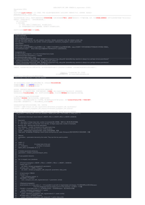
吴恩达深度学习第⼆课第⼀周编程作业_regularization(正则化)Regularization 正则化声明本⽂作业是在jupyter notebook上⼀步⼀步做的,带有⼀些过程中查找的资料等(出处已标明)并翻译成了中⽂,如有错误,欢迎指正!参考Kulbear 的和和,以及的,以及,欢迎来到本周的第⼆次作业。
深度学习模型有很⼤的灵活性和容量,如果训练数据集不够⼤,过拟合可能会成为⼀个严重的问题。
当然,它在训练集上做得很好,但学习过的⽹络不能推⼴到它从未见过的新例⼦!(也就是训练可以,⼀到实战测试就拉胯。
) 第⼆个作业的⽬的: 2. 正则化模型: 2.1:使⽤⼆范数对⼆分类模型正则化,尝试避免过拟合。
2.2:使⽤随机删除节点的⽅法精简模型,同样是为了尝试避免过拟合。
您将学习:在您的深度学习模型中使⽤正则化。
让我们⾸先导⼊将要使⽤的包。
# import packagesimport numpy as npimport matplotlib.pyplot as pltfrom reg_utils import sigmoid, relu, plot_decision_boundary, initialize_parameters, load_2D_dataset, predict_decfrom reg_utils import compute_cost, predict, forward_propagation, backward_propagation, update_parametersimport sklearnimport sklearn.datasetsimport scipy.io #scipy是构建在numpy的基础之上的,它提供了许多的操作numpy的数组的函数。
scipy.io包提供了多种功能来解决不同格式的⽂件的输⼊和输出。
from testCases import * #from XXX import*是把XXX下的所有名字引⼊当前名称空间。
Dynaform5.9BSE培训资料

坯料展开及排样
本教程通过Coat Hanger零件来描述 坯料尺寸展开计算以及排样的过程
I. 新建和保存数据库
1. 启动 Dynaform 5.9。 2. 单击文件菜单,选择另存为…子菜单(如图1所示)。 3. 输入“BSE_(user name)_(date).df ” 作为文件名。 4. 单击保存按钮保存数据库。
中(如图 26所示)。 3. 单击新建按钮在列表中新建一组轮廓(如图27所示)。 4. 单击导入线图标,并选择导入outline2.igs(如图28和29所示)。 5. 切换到Outline1组坯料轮廓线,程序自动切换当前显示的内容,把
Outline2 零件层关闭。 6. 单击 保存数据库。
20
VIII.坯料轮廓线管理
23
IX. 坯料排样
图 30
图 31
图 32
24
8. 察看排样结果
排样计算完成后,所有可能的排样结果都显示 在结果列表中。图形区中缺省显示的是在当前的 限制条件下,材料利用率最大的排样结果。用户 可以单击结果列表中的其他结果,在图形区中显 示出来。同时也可以返回到前面来详细的设置参 数,重新计算排样。如图33、图34所示。
图 13
10
V. 自动曲面网格划分
1. 选择 坯料工程 预处理 。 2. 切换到网格页面,选择曲面网格划分 (如图 14所示) 。 3. 系统默认的网格为Mstep Mesh,同时默认选中当前sheet工具中所有零
件层的曲面(如图15所示) 。 4. 在参数中输入最大尺寸, 2.00 (mm) 。 5. 单击按钮应用进行网格划分。 6. 单击是接受划分的网格。 7. 单击退出按钮退出曲面网格划分对话框。 8. 如图16所示 。
gromacs tutorial
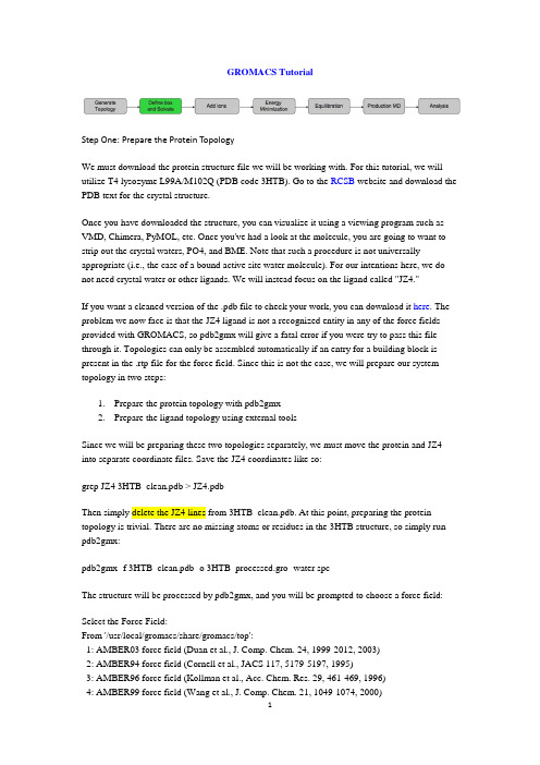
GROMACS TutorialStep One: Prepare the Protein TopologyWe must download the protein structure file we will be working with. For this tutorial, we will utilize T4 lysozyme L99A/M102Q (PDB code 3HTB). Go to the RCSB website and download the PDB text for the crystal structure.Once you have downloaded the structure, you can visualize it using a viewing program such as VMD, Chimera, PyMOL, etc. Once you've had a look at the molecule, you are going to want to strip out the crystal waters, PO4, and BME. Note that such a procedure is not universally appropriate (i.e., the case of a bound active site water molecule). For our intentions here, we do not need crystal water or other ligands. We will instead focus on the ligand called "JZ4."If you want a cleaned version of the .pdb file to check your work, you can download it here. The problem we now face is that the JZ4 ligand is not a recognized entity in any of the force fields provided with GROMACS, so pdb2gmx will give a fatal error if you were try to pass this file through it. Topologies can only be assembled automatically if an entry for a building block is present in the .rtp file for the force field. Since this is not the case, we will prepare our system topology in two steps:1.Prepare the protein topology with pdb2gmx2.Prepare the ligand topology using external toolsSince we will be preparing these two topologies separately, we must move the protein and JZ4 into separate coordinate files. Save the JZ4 coordinates like so:grep JZ4 3HTB_clean.pdb > JZ4.pdbThen simply delete the JZ4 lines from 3HTB_clean.pdb. At this point, preparing the protein topology is trivial. There are no missing atoms or residues in the 3HTB structure, so simply run pdb2gmx:pdb2gmx -f 3HTB_clean.pdb -o 3HTB_processed.gro -water spcThe structure will be processed by pdb2gmx, and you will be prompted to choose a force field:Select the Force Field:From '/usr/local/gromacs/share/gromacs/top':1: AMBER03 force field (Duan et al., J. Comp. Chem. 24, 1999-2012, 2003)2: AMBER94 force field (Cornell et al., JACS 117, 5179-5197, 1995)3: AMBER96 force field (Kollman et al., Acc. Chem. Res. 29, 461-469, 1996)4: AMBER99 force field (Wang et al., J. Comp. Chem. 21, 1049-1074, 2000)5: AMBER99SB force field (Hornak et al., Proteins 65, 712-725, 2006)6: AMBER99SB-ILDN force field (Lindorff-Larsen et al., Proteins 78, 1950-58, 2010)7: AMBERGS force field (Garcia & Sanbonmatsu, PNAS 99, 2782-2787, 2002)8: CHARMM27 all-atom force field (with CMAP) - version 2.09: GROMOS96 43a1 force field10: GROMOS96 43a2 force field (improved alkane dihedrals)11: GROMOS96 45a3 force field (Schuler JCC 2001 22 1205)12: GROMOS96 53a5 force field (JCC 2004 vol 25 pag 1656)13: GROMOS96 53a6 force field (JCC 2004 vol 25 pag 1656)14: OPLS-AA/L all-atom force field (2001 aminoacid dihedrals)15: [DEPRECATED] Encad all-atom force field, using full solvent charges16: [DEPRECATED] Encad all-atom force field, using scaled-down vacuum charges17: [DEPRECATED] Gromacs force field (see manual)18: [DEPRECATED] Gromacs force field with hydrogens for NMRFor this tutorial, we will use the united-atom GROMOS96 43A1 force field, so type 9 at the command prompt, followed by 'Enter'Step Two: Prepare the Ligand TopologyFor this tutorial, we will use PRODRG to generate a starting topology for our ligand, JZ4. Go to the PRODRG site and upload your JZ4.pdb file. The server presents you with several options for how to treat your ligand:∙Chirality (yes/no): maintain chiral centers in the input molecule (yes), or reconstruct them (no). In our case, we have no chirality, so leave this option set to its default.∙Charges (full/reduced): full charges are for condensed-phase systems (43A1 force field);reduced are for "vacuum" simulations (43B1 force field). Use full charges for nearly allapplications. The accuracy of 43B1 is debatable, anyway.∙EM (yes/no): perform energy minimization (yes), or leave coordinates alone (no). In our case, we want to construct our protein-ligand complex from existing coordinates, so wedo not want PRODRG to minimize our molecule in vacuo. Choose "no" for this option.∙Force field (GROMOS96.1/GROMOS87): "GROMOS96.1" refers to the first version of the GROMOS96 force field, 43A1. "GROMOS87" refers to the (outdated!) GROMOS87 force field. Choose "GROMOS96.1" to get 43A1 parameters for our ligand.We will make use of two files that PRODRG gives us. Save the output of the field "The GROMOS87/GROMACS coordinate file (polar/aromatic hydrogens)" into a text file called"jz4.gro" and "The GROMACS topology" into a file called "drg.itp."Let's take a look at the [ atoms ] section of our JZ4 topology:[ atoms ]; nr type resnr resid atom cgnr charge mass1 CH3 1 JZ4 C4 1 0.000 15.03502 CH2 1 JZ4 C14 2 0.059 14.02703 CH2 1 JZ4 C13 2 0.060 14.02704 C 1 JZ4 C12 2 -0.041 12.01105 CR1 1 JZ4 C11 2 -0.026 12.01106 HC 1 JZ4 H11 2 0.006 1.00807 CR1 1 JZ4 C7 2 -0.026 12.01108 HC 1 JZ4 H7 2 0.006 1.00809 CR1 1 JZ4 C8 2 -0.026 12.011010 HC 1 JZ4 H8 2 0.007 1.008011 CR1 1 JZ4 C9 2 -0.026 12.011012 HC 1 JZ4 H9 2 0.007 1.008013 C 1 JZ4 C10 3 0.137 12.011014 OA 1 JZ4 OAB 3 -0.172 15.999415 H 1 JZ4 HAB 3 0.035 1.0080I immediately notice three things that are wrong with this topology:1.Charge group 2 encompasses the entire aromatic ring, nearly all of the atoms in thismolecule.2.Charges of equivalent functional groups (C-H) are not uniform. In some cases, H atomsare +0.006e, and in other cases they are +0.007e.3.Charges on these atoms bear no resemblance whatsoever to the expected chargesprescribed by the force field.So what do we do? If you read the paper linked above, you would know what I'm going to recommend already. Assign charges and charge groups from equivalent functional groups in a building block-style manner. For any unknown groups, perform the charge calculations suggested in the paper. Since JZ4 involves only functional groups found in proteins (hydrophobic chain, aromatic ring, and an alcohol), life is pretty easy. We can re-assign charges and charge groups from these moieties. I will not go into proper topology validation in this tutorial; it would be far too time-consuming. Suffice it to say that you must satisfy reviewers that the parameters applied to your molecule are reliable. They should reproduce some well-known observable, such as logP or ΔG hydr, as in the GROMOS96 literature. If you cannot satisfy these requirements for your own system, you may want to reconsider your choice of force field.I would construct a topology that has something like this for an [ atoms ] directive:[ atoms ]; nr type resnr resid atom cgnr charge mass1 CH3 1 JZ4 C4 1 0.000 15.03502 CH2 1 JZ4 C14 2 0.000 14.02703 CH2 1 JZ4 C13 2 0.000 14.02704 C 1 JZ4 C12 2 0.000 12.01105 CR1 1 JZ4 C11 3 -0.100 12.01106 HC 1 JZ4 H11 3 0.100 1.00807 CR1 1 JZ4 C7 4 -0.100 12.01108 HC 1 JZ4 H7 4 0.100 1.00809 CR1 1 JZ4 C8 5 -0.100 12.011010 HC 1 JZ4 H8 5 0.100 1.008011 CR1 1 JZ4 C9 6 -0.100 12.011012 HC 1 JZ4 H9 6 0.100 1.008013 C 1 JZ4 C10 7 0.150 12.011014 OA 1 JZ4 OAB 7 -0.548 15.999415 H 1 JZ4 HAB 7 0.398 1.0080Note that equivalent functional groups have equivalent charges, hydrophobic groups are completely uncharged, and the charge groups are of a sensible size (2-3 atoms). The other elements of the topology are sufficiently accurate. Bonded parameters assigned by PRODRG are generally reliable. We are now ready to construct the system topology and reconstruct our protein-ligand complex.Build the ComplexFrom pdb2gmx, we have a file called "conf.gro" that contains the processed, force field-compliant structure of our protein. We also have "jz4.gro" from PRODRG that has included all of the necessary H atoms. Simply copy the coordinate section of jz4.gro and paste it into conf.gro, below the last line of the protein atoms, and before the box vectors, like so:163ASN C 1691 0.621 -0.740 -0.126163ASN O1 1692 0.624 -0.616 -0.140163ASN O2 1693 0.683 -0.703 -0.0115.99500 5.19182 9.66100 0.00000 0.00000 -2.99750 0.00000 0.00000 0.00000becomes (added text in bold green)...163ASN C 1691 0.621 -0.740 -0.126163ASN O1 1692 0.624 -0.616 -0.140163ASN O2 1693 0.683 -0.703 -0.0111JZ4 C4 1 2.429 -2.412 -0.0071JZ4 C14 2 2.392 -2.470 -0.1391JZ4 C13 3 2.246 -2.441 -0.1811JZ4 C12 4 2.229 -2.519 -0.3081JZ4 C11 5 2.169 -2.646 -0.2951JZ4 H11 6 2.135 -2.683 -0.1991JZ4 C7 7 2.155 -2.721 -0.4111JZ4 H7 8 2.104 -2.817 -0.4071JZ4 C8 9 2.207 -2.675 -0.5331JZ4 H8 10 2.199 -2.738 -0.6211JZ4 C9 11 2.267 -2.551 -0.5451JZ4 H9 12 2.306 -2.516 -0.6401JZ4 C10 13 2.277 -2.473 -0.4301JZ4 OAB 14 2.341 -2.354 -0.4341JZ4 HAB 15 2.369 -2.334 -0.5285.99500 5.19182 9.66100 0.00000 0.00000 -2.99750 0.00000 0.00000 0.00000Since we have added 15 more atoms into the .gro file, increment the second line of conf.gro to reflect this change. There should be 1708 atoms in the coordinate file now.Build the TopologyIncluding the parameters for the JZ4 ligand in the system topology is very easy. Just insert a line that says #include "drg.itp" into topol.top after the position restraint file is included. The inclusion of position restraints indicates the end of the "Protein" moleculetype section.; Include Position restraint file#ifdef POSRES#include "posre.itp"#endif; Include water topology#include "gromos43a1.ff/spc.itp"becomes...; Include Position restraint file#ifdef POSRES#include "posre.itp"#endif; Include ligand topology#include "drg.itp"; Include water topology#include "gromos43a1.ff/spc.itp"The last adjustment to be made is in the [ molecules ] directive. To account for the fact that there is a new molecule in conf.gro, we have to add it here, like so:[ molecules ]; Compound #molsProtein_chain_A 1JZ4 1The topology and coordinate file are now in agreement with respect to the contents of the system. Step Three: Defining the Unit Cell & Adding SolventAt this point, the workflow is just like any other MD simulation. We will define the unit cell andfill it with water.editconf -f conf.gro -o newbox.gro -bt dodecahedron -d 1.0genbox -cp newbox.gro -cs spc216.gro -p topol.top -o solv.groStep Four: Adding IonsWe now have a solvated system that contains a charged protein. The output of pdb2gmx told us that the protein has a net charge of +6e (based on its amino acid composition). If you missed this information in the pdb2gmx output, look at the last line of your [ atoms ] directive in topol.top; it should read (in part) qtot。
python-tutorial

The Python interpreter and the extensive standard library are freely available in source or binary form for all major platforms from the Python web site, , and can be freely distributed. The same site also contains distributions of and pointers to many free third party Python modules, programs and tools, and additional documentation.
CONTENTS
1 Whetting Your Appetite
1
1.1 Where From Here . . . . . . . . . . . . . . . . . . . . . . . . . . . . . . . . . . . . . . . . . . . . 2
2 Using the Python Interpreter
neural network training(nntraintool) 的使用说明
neural network training(nntraintool) 的使用说明`nntraintool` 是一个MATLAB 中用于神经网络训练的工具。
它提供了一个交互式界面,可以帮助用户设置和控制训练过程。
以下是使用`nntraintool` 的一般步骤:1. 在MATLAB 中加载数据集并创建神经网络模型。
2. 使用`nntool` 命令打开`nntraintool` 工具:```matlabnntool```3. 在`nntraintool` 界面中,选择要训练的神经网络模型。
如果之前已经在MATLAB 中创建了模型,则可以从下拉菜单中选择该模型。
4. 设置训练参数:-Epochs(迭代次数):设置训练迭代的次数。
每个epoch 表示将所有训练样本都用于训练一次。
- Learning Rate(学习率):控制权重和偏差调整的速度。
较高的学习率可以加快收敛速度,但可能导致不稳定的训练结果;较低的学习率可以增加稳定性,但可能导致收敛速度变慢。
- Momentum(动量):控制权重更新的惯性,有助于跳出局部最小值。
较高的动量可以加速收敛,但可能导致超调现象。
- Validation Checks(验证检查):设置多少个epoch 进行一次验证,用于监控训练过程的性能。
- Performance Goal(性能目标):设置期望的训练误差。
5. 点击"Train" 按钮开始训练。
`nntraintool` 将显示每个epoch 的训练进度和性能曲线。
6. 在训练过程中,你可以使用`nntraintool` 提供的功能来监视训练进度和性能。
例如,你可以查看误差曲线、性能曲线和权重变化。
7. 训练完成后,你可以保存已训练的神经网络模型,以便后续使用。
以上是使用`nntraintool` 的基本步骤。
请注意,在实际使用中,你可能需要根据你的特定问题和数据集进行适当的调整和优化。
此外,MATLAB 官方文档提供了更详细的说明和示例,可以帮助你更深入地了解如何使用`nntraintool` 进行神经网络训练。
Part3

2.
3.
铺铜及内电层 ............................................................................................................................6 1.1 铺铜及铺铜管理器 ...........................................................................................................6 1.1.1 放置铺铜.............................................................................................................6 1.1.2 设置网格铺铜的拐角模式(仅对网格铺铜) ......................................................8 1.1.3 编辑铺铜.............................................................................................................8 1.1.5 切断铺铜区 .........................................................................................................9 1.1.6 隐藏铺铜..................................................................................
bsr训练方法
bsr训练方法
BSR(Bilingual Sentence Representation)是一种训练方法,用
于将双语句子映射到一个高维的共享语义空间中的相似表示。
BSR的训练方法主要包括以下步骤:
1. 数据准备:首先需要准备成对的双语语料数据,包括源语言句子和目标语言句子。
2. 双语句子对齐:使用对齐工具将双语句子进行对齐,确保每个源语言句子都能找到对应的目标语言句子。
3. 双语句子编码器:建立一个双语句子编码器,它能够将源语言句子和目标语言句子分别映射到一个共享的语义空间中的表示。
4. 双语句子对损失函数:定义一个双语句子对损失函数,用来度量源语言句子和目标语言句子的相似度。
5. 迭代训练:使用双语句子对损失函数对编码器进行优化训练,通过反向传播算法更新参数,使得源语言句子和目标语言句子在共享语义空间中的表示能够更加接近。
6. 相似度计算:在训练过程中,可以使用一些相似度计算方法,比如余弦相似度,来度量不同句子在共享语义空间中的相似程度。
7. 性能评估:使用一些评估指标,比如准确率、召回率等,来
评估训练出的双语句子表示在不同任务上的性能。
通过以上步骤,BSR训练方法可以得到一个高质量的双语句子表示,这种表示能够在多个自然语言处理任务中发挥作用,比如机器翻译、文本对齐、语义匹配等。
- 1、下载文档前请自行甄别文档内容的完整性,平台不提供额外的编辑、内容补充、找答案等附加服务。
- 2、"仅部分预览"的文档,不可在线预览部分如存在完整性等问题,可反馈申请退款(可完整预览的文档不适用该条件!)。
- 3、如文档侵犯您的权益,请联系客服反馈,我们会尽快为您处理(人工客服工作时间:9:00-18:30)。
Figure 26
Figure 27
Figure 28
17
�
11
IV. Check and Repair Mesh
Figure 12 Figure 15
Figure 13 Figure 14 Figure 16
12
V. Blank Size Estimate
1. 2. Select BSE Preparation Blank Size Estimate (See Figure 17). Click Null in the displayed blank size estimate window to define material (See Figure 18). 3. Click Material Library in the displayed material window (See Figure 19). 4. Select CQ (mild) as the material (See Figure 20). 5. Click OK to exit MATERIAL TYPE 36 dialog box (See Figure 21). 6. Click OK to exit Material dialog box (See Figure 22). 7. Automatically enter the part Thickness: 3.20 (mm) (See Figure 23). 8. Click Apply to run BSE (See Figure 24). 9. Click Exit to dismiss BSE Preparation dialog box. 10. Click to open the Display Part dialog box. 11. Select MIDSRF 1 and click OK to close part MIDSRF 1, with OUT Line displayed only. 12. Click to display the blank outline in TOP view (See Figure 25). 13. Click to save the database.
9
III. Mesh
Figure 9
Figure 11 Figure 10
10
IV. Check and Repair Mesh
1. Toggle off Surface (See Figure 12). 2. Select Model Check/Repair (See Figure 13). 3. Click Boundary Display icon(the second icon in the first row)(See Figure 14). 4. Toggle off Elements and Node. 5. Click (free rotation) to rotate the model. 6. Click (clear highlight). 7. Click to display the model in isometric view. 8. Click Auto Normal icon (the first icon in the first row). 9. Select CURSOR PICK PART 10. Move the cursor to select an element on the model (See Figure 15). 11. Select No to reverse the normal direction (See Figure 16). 12. Click Exit to dismiss the dialog box. 13. Click OK to exit Model Check/Repair dialog box.
13
V. Blank Size Estimate
Figure 17
Figure 19
Figure 20 Figure 18
பைடு நூலகம்
14
V. Blank Size Estimate
Figure 21
Figure 22
Figure 23
15
V. Blank Size Estimate
Figure 24
Figure 25
3
I. Open and save database
Figure 1
Figure 2
4
I. Open and save database
Figure 3
Figure 4
5
I. Open and save database
Figure 5
6
II. Middle Surface
1. Click BSE Preparation menu. 2. Click Middle Surface button (the third button in the first row), as shown in Figure 6. 3. The program pops up the Select Surfaces window. Click Displayed Surf to select all the displayed surfaces. 4. Click OK to calculate the middle surface of part automatically. Click Done to exit. 5. Click Part Turn On/Off button. The middle surface is automatically named as MidSrf1. (See Figure 8).
DYNAFORM 5.7 Training Tutorial
Mid surface and Separate surface
Descriptions of BSE blank unfolding function for models with thickness by using MidSurface part.
Figure 6 Figure 7
7
II. Middle Surface
Figure 8
8
III. Mesh
1. Toggle off the original Product part and keep the middle surface MidSrf1 only. Click on Current Part at the lower right corner and set MidSrf1 as the current part. 2. Click BSE Preparation menu. 3. Click Part Mesh button (See Figure 9). 4. Click Select Surfaces in the displayed Surface Mesh window (See Figure 10). 5. Click Displayed Surf to select middle surfaces and click OK to exit. 6. Type in the mesh max. Size:2mm 7. Click Apply to mesh. 8. Click OK to exit Mesh Quality Check window. 9. Click Yes to confirm the generated mesh (See Figure 11). 10. Click Exit to dismiss the Surface Mesh window.
I. Open and save database
1. 2. 3. 4. 5. 6. Start up Dynaform 5.7. Click File Open and select Midsurface.df file. Click File Save As (See Figure 3). Enter Midsurface_(user name)_(date).df as the file name. Click Save to save the database. The data model is shown in Figure 5. The part name is PRODUCT and the model is a part with thickness. The user needs to take out middle surface first and then use Mstep function to unfold.
16
Description about BSE Separate Surface
BSE Preparation Separate Surface can automatically separate the imported model with thickness into three parts: top surface, bottom surface and the surface along part thickness direction. Description for a case of midsurface.df is given below: Click Group Surface button and press Displayed Surf to select the entire model with thickness. Click OK to separate the model into three parts: ThkSrf1, TopSrf 1 and BotSrf 1.