北京理工大学 自动控制原理考研 ppt课件
合集下载
《自动控制原理》PPT课件
4
4-1 根轨迹的基本概念
4-1-1 根轨迹
闭环极点随开环根轨迹增益变化的轨迹
目标
系统参数 连续、运动、动态
开环系统中某个参数由0变化到 时,
闭环极点在s平面内画出的轨迹。一 个根形成一条轨迹。
5
例4-1 已知系统如图,试分析 Kc 对系统特征根分布的影响。
R(s)
_ Kc
1
C(s)
s(s+2)
解:开环传递函数 G(s) Kc 开环极点:p1 0
s(s 2)
开环根轨迹增益:K * Kc 闭环特征方程:s2 2s K * 0
闭环特征根
2 s1,2
4 4K* 1
2
1 K*
p2 2
6
研究K*从0~∞变化时,闭环特征根的变化
K*与闭环特征根的关系 s1,2 1 1 K*
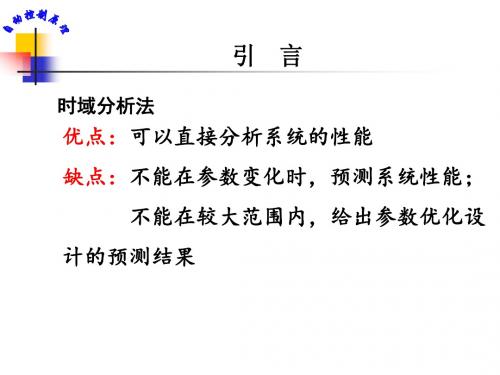
引言
时域分析法
优点:可以直接分析系统的性能 缺点:不能在参数变化时,预测系统性能;
不能在较大范围内,给出参数优化设 计的预测结果
系统的闭环极点
系统的稳定性 系统的动态性能
系统闭环特征方程的根
高阶方程情形 下求解很困难
系统参数(如开环放大倍数)的变化会引起其 变化,针对每个不同参数值都求解一遍根很麻 烦。
1 绘制依据 ——根轨迹方程
R(s) _
C(s) G(s)
闭环的特征方程:1 G(s)H(s) 0
H(s)
即:G(s)H(s) 1 ——根轨迹方程(向量方程)
用幅值、幅角的形式表示:
G(s)H(s) 1
G(s)H(s) [G(s)H(s)] 1(2k 1) G(s)H(s) (2k 1)
4-1 根轨迹的基本概念
4-1-1 根轨迹
闭环极点随开环根轨迹增益变化的轨迹
目标
系统参数 连续、运动、动态
开环系统中某个参数由0变化到 时,
闭环极点在s平面内画出的轨迹。一 个根形成一条轨迹。
5
例4-1 已知系统如图,试分析 Kc 对系统特征根分布的影响。
R(s)
_ Kc
1
C(s)
s(s+2)
解:开环传递函数 G(s) Kc 开环极点:p1 0
s(s 2)
开环根轨迹增益:K * Kc 闭环特征方程:s2 2s K * 0
闭环特征根
2 s1,2
4 4K* 1
2
1 K*
p2 2
6
研究K*从0~∞变化时,闭环特征根的变化
K*与闭环特征根的关系 s1,2 1 1 K*
引言
时域分析法
优点:可以直接分析系统的性能 缺点:不能在参数变化时,预测系统性能;
不能在较大范围内,给出参数优化设 计的预测结果
系统的闭环极点
系统的稳定性 系统的动态性能
系统闭环特征方程的根
高阶方程情形 下求解很困难
系统参数(如开环放大倍数)的变化会引起其 变化,针对每个不同参数值都求解一遍根很麻 烦。
1 绘制依据 ——根轨迹方程
R(s) _
C(s) G(s)
闭环的特征方程:1 G(s)H(s) 0
H(s)
即:G(s)H(s) 1 ——根轨迹方程(向量方程)
用幅值、幅角的形式表示:
G(s)H(s) 1
G(s)H(s) [G(s)H(s)] 1(2k 1) G(s)H(s) (2k 1)
北理工自动控制理论课件
t
cmax = sup |c(t)|,0 ≤ t ≤ ∞
调整时间 上升时间
§5 自动控制系统的研究方法
• 自动控制研究的三个基本问题: 建立数学模型 系统性能分析 控制器设计 • 分析: 在给定系统的条件下,将物理系统抽象成数学模型, 然 后用已经成熟的数学方法和先进的计算工具来定性或定量地 对系统进行动、静态的性能分析。 • 综合: 在已知被控对象和合定性能指标的前提下,寻求控制规 律,建立一个能使被控对象满足性能要求的系统。
三.自动控制技术的作用 1. 自动控制技术的应用不仅使生产过程实 现了自动化,极大地提高了劳动生产率, 而且减轻了人的劳动强度。 2. 自动控制使工作具有高度的准确性,大 大地提高了武器的命中率和战斗力,例如 火炮自动跟踪系统必须采用计算机控制才 能打下高速高空飞行的飞机。 3. 某些人们不能直接参与工作的场合就更离 不开自动控制技术了,例如原子能的生产、 火炮或导弹的制导等等。
控制系统的工作原理 1.人工控制恒温箱温度
控制过程: 1 观测恒温箱中的温度(被控 量) 2 与要求的温度(给定值)进 行比较得到温度偏差的大小和 方向 3 根据偏差大小和方向调节调 压器,控制加热电阻丝的电流 以调节温度回复到要求的温度
控制流程如图:
控制的实质:检测偏差和纠正偏差
2 恒温箱自动控制系统
•
美国的M. E. Merchant 提出计算机集成制造 的概念(1969);
•
日本Fanuc 公司研制出由加工中心和工业机 器人组成的柔性制造单元(1976);
中国批准 863高技术计划,包括自动化领域的 计算机集成制造系统和智能机器人两个主题 (1986)。
• 日本安川公司娱制 控制装置与被控对象之间只有顺向作用 而没有反向联系的控制。
《自动控制原理》PPT课件_OK
例如对一个微分方程,若已知初值和输入值,对 微分方程求解,就可以得出输出量的时域表达式。 据此可对系统进行分析。所以建立控制系统的数学 模型是对系统进行分析的第一步也是最重要的一步。
控制系统如按照数学模型分类的话,可以分为线 性和非线性系统,定常系统和时变系统。
2021/7/21
2
自动控制原理
[线性系统]:如果系统满足叠加原理,则称其为线性系 统。叠加原理说明,两个不同的作用函数同时作用于 系统的响应,等于两个作用函数单独作用的响应之和。
[解]速度控制系统微分方程为:
a2 a1 a0 b1ug b0ug 对上式各项进行拉氏变换,得:
(s)(a2s2 a1s a0) Ug (s)(b1s b0)
即:
(s)
(b1s (a2s2
b0 ) a1s
a0 )
U
g
(s)
当输入已知时,求上式的拉氏反变换,即可求得输出
的时域解。
2021/7/21
2021/7/21
20
自动控制原理
[关于传递函数的几点说明]
❖ 传递函数的概念适用于线性定常系统,与线性常系 数微分方程一一对应。与系统的动态特性一一对应。
❖ 传递函数不能反映系统或元件的学科属性和物理性 质。物理性质和学科类别截然不同的系统可能具有 完全相同的传递函数。而研究某传递函数所得结论 可适用于具有这种传递函数的各种系统。
将上式求拉氏变化,得(令初始值为零)
(ansn an1sn1 a1s a0)Y(s) (bmsm bm1sm1 b1s b0)X (s)
G(s)
Y (s) X (s)
bm s m an s n
bm1sm1 b1s b0 an1sn1 a1s a0
北京理工大学810自动控制原理考研课件9

K L( s ) (10s 1)(2s 1)(0.2 s 1)
determine the stability of the system at K=20 and K=100.
14
1. start: lim L( j ) lim K K 0
0 0
2. end: lim L ( j )=0 270
n i 1 M
(s p )
k 1 k
• The poles of F(s) are the poles of L(s). • The zeros of F(s) are the characteristic roots of the system.
9
• For a system to be stable, all the zeros of F(s) must lie in the left-hand s-plane. • Choose a contour Γ s in the s-plane that encloses the entire right-hand s-plane, the number of encirclements of the origin of the j F(s)-plane is N=Z-P. Z: zeros in RHP P: poles in RHP r=∞ • So the number of unstable 0 poles of the system is Z=N+P
5
7.2 Mapping Contours in the s-plane
• A contour map is a contour in one plane mapped into another plane by a relation F(s). Example: s
自动控制原理24 24页PPT文档

-
1
1 uo(s)
R 2 I2(s) C 2 s
为了求出总的传递函数,需要进行适当的等效变换。一个
可能的变换过程如下:
C2s
ui (s) -
1 I1(s) - 1 u (s)
R1
I(s) C1s
1 R2C2s 1
uo(s) ①
ui (s) -
9/8/2019
-1
R1
R1C2s
1
u(s)
C1s
1 R2C2s 1
9/8/2019
20Leabharlann 动输入作用下的闭环系统的传递函数(二)扰动作用下的闭环系统:
此时R(s)=0,结构图如下:
N (s)
E(s)
+
G1(s)
G2 (s)
-
B(s) H (s)
输出对扰动的传递函数为:
C(s)
N(s)C N((ss))1G G 21(G s)2H
输出为:C(s) G2 N(s) 1G1G2H
u f (s)
Kf
- (s)
在结构图中,不仅能反映系统的组成和信号流向,还能表 示信号传递过程中的数学关系。系统结构图也是系统的数学模 型,是复域的数学模型。
9/8/2019
5
结构图的等效变换
二、结构图的等效变换: [定义]:在结构图上进行数学方程的运算。 [类型]:①环节的合并;
--串联 --并联 --反馈连接 ②信号分支点或相加点的移动。 [原则]:变换前后环节的数学关系保持不变。
①信号相加点的移动:
把相加点从环节的输入端移到输出端
X1(s)
G(s) Y (s)
X2(s)
X1(s) G(s) X2(s) N (s)
自动控制原理课件ppt

G3(s)
G2(s)
H3(s)
E(S)
R(s)
G1(s)
H1(s)
H2(s)
C(s)
P2= - G3G2H3
△2= 1
P2△2=
梅逊公式求E(s)
P1= –G2H3
△1= 1
N(s)
G1(s)
H1(s)
H2(s)
C(s)
G3(s)
G2(s)
H3(s)
R(s)
E(S)
四个单独回路,两个回路互不接触
e
A
100%
一阶系统时域分析
无零点的一阶系统 Φ(s)=
Ts+1
k
, T
时间常数
(画图时取k=1,T=0.5)
单 位 脉 冲 响 应
k(t)=
T
1
e-
T
t
k(0)=
T
1
K’(0)=
T
1
2
单位阶跃响应
h(t)=1-e-t/T
h’(0)=1/T
h(T)=0.632h(∞)
h(3T)=0.95h(∞)
h(2T)=0.865h(∞)
第一章 自动控制的一般概念
1-1 自动控制的基本原理与方式 1-2 自动控制系统示例 1-3 自动控制系统的分类 1-4 对自动控制系统的基本要求
飞机示意图
给定电位器
反馈电位器
给定装置
放大器
舵机
飞机
反馈电位器
垂直陀螺仪
θ0
θc
扰动
俯仰角控制系统方块图
飞机方块图
液位控制系统
控制器
自动控制原理课件ppt
课件3 ~6为第一章的内容。制作目的是节省画图时间,便于教师讲解。 课件6要强调串联并联反馈的特征,在此之前要交待相邻综合点与相邻引出点的等效变换。 课件7中的省略号部分是反过来说,如‘合并的综合点可以分开’等。最后一条特别要讲清楚,这是最容易出错的地方! 课件10先要讲清H1和H3的双重作用,再讲分解就很自然了。 课件11 、12 、13是直接在结构图上应用梅逊公式,制作者认为没必要将结构图变为信号流图后再用梅逊公式求传递函数。
自动控制原理(全套课件659P)

手动控制
人在控制过程中起三个作用: (1)观测:用眼睛去观测温度计和转速表的指示值;
(2)比较与决策:人脑把观测得到的数据与要求的数据相比较,并进行
判断节,如调节阀门开度、改变触点位置。
ppt课件 4
1.1 自动控制的基本概念
在现代科学技术的众多领域中,自动控制技术起着越来越重要的作用。 如数控车床按预定程序自动切削,人造卫星准确进入预定轨道并回收
ppt课件 6
控制系统分析:已知系统的结构参数,分析系统的稳定性,求取系
统的动态、静态性能指标,并据此评价系统的过程称为控制系统分 析。
控制系统设计(或综合):根据控制对象和给定系统的性能指标,
合理的确定控制装置的结构参数,称为控制系统设计。 被控量 :指被控对象中要求保持给定值、要按给定规律变化的物理 量。被控量又称输出量、输出信号 。 给定值:系统输出量应达到的数值(例如与要求的炉温对应的电 压)。 扰动:是一种对自动控制系统输出量起反作用的信号,如电源电压
闭环控制是指系统的被控制量(输出量)
与控制作用之间存在着负反馈的控制 方式。采用闭环控制的系统称为闭环
控制系统或反馈控制系统。闭环控制
是一切生物控制自身运动的基本规律。 人本身就是一个具有高度复杂控制能
力的闭环系统。
优点:具有自动补偿由于系统内部和外 部干扰所引起的系统误差(偏差)的
能力,因而有效地提高了系统的精度。
脑
手
输出量 (手的位置)
ppt课件
16
闭环控制系统方框图
ppt课件
17
反馈控制系统的组成、名词术语和定义
反馈控制系统方框图
ppt课件
18
1.2 自动控制理论的发展
《自动控制原理》PPT课件
i1
j1
i1
j1
f
G(s)
K G (1s 1)(22s2 22s 1) s (T1s 1)(T22s2 2T2s 1)
KG'
(s zi )
i1 q
(s pi )
i1
前向通道增益 前向通道根轨迹增益
KG'
KG
1 2 2 T1T2 2
反馈通道根轨迹增益
l
(s z j )
H(s) K H '
狭义根轨迹(通常情况):
变化参数为开环增益K,且其变化取值范围为0到∞。
G(s)H (s) K s(s 1)
(s) C(s) K R(s) s2 s K
D(s) s2 s K 0
s1,2
1 2
1 2
1 4K
K=0时 s1 0 s2 1
0 K 1/ 4 两个负实根
K值增加 相对靠近移动
i1
i1
负实轴上都是根轨迹上的点!
m
n
(s zi ) (s pi ) | s2 p1 135
i1
i1
负实轴外的点都不是根轨迹上的点!
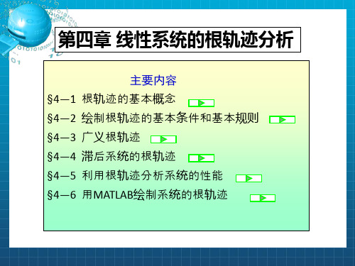
二、绘制根轨迹的基本规则
一、根轨迹的起点和终点 二、根轨迹分支数 三、根轨迹的连续性和对称性 四、实轴上的根轨迹 五、根轨迹的渐近线 六、根轨迹的分离点 七、根轨迹的起始角和终止角 八、根轨迹与虚轴的交点 九、闭环特征方程根之和与根之积
a
(2k 1)180 nm
渐近线与实轴交点的坐标值:
n
m
pi zi
a= i1
i1
nm
证明
G(s)H (s) K '
m
(s zi )
i 1 n
- 1、下载文档前请自行甄别文档内容的完整性,平台不提供额外的编辑、内容补充、找答案等附加服务。
- 2、"仅部分预览"的文档,不可在线预览部分如存在完整性等问题,可反馈申请退款(可完整预览的文档不适用该条件!)。
- 3、如文档侵犯您的权益,请联系客服反馈,我们会尽快为您处理(人工客服工作时间:9:00-18:30)。
4
Root Locus
unstable
4
K
3 G(s) s2 (s 2)
2
1
Imag Axis
0
-1
-2
-3
-4
-6
-5
-4
-3
-2
-1
0
1
2
Real Axis
5
理硕教育—专注于北理工考研辅 导
• 本资料由理硕教育整理,理硕教育是全国 唯一专注于北理工考研辅导的学校,相对 于其它机构理硕教育有得天独厚的优势。 丰富的理工内部资料资源与人力资源确保 每个学员都受益匪浅,确保理硕教育的学 员初试通过率89%以上,复试通过率接近 100%,理硕教育现开设初试专业课VIP一 对一,初试专业课网络小班,假期集训营 ,复试VIP一对一辅导,复试网络小班,考 前专业课网络小班,满足学员不同的需求 6
compensated root locus.
5. Evaluate the total system gain at the desired root
location and then calculate the error constant.
6. If the error constant is not satisfactory, a Phase-lag
R(s) Gc(s) + -
Y(s) G(s)
H(s)
(d) Input compensation
3
2. Phase-lead design using the root locus Adding a single zero moves root locus to
the left and achieves the higher stability.
Chapter 5 Root Locus Method
5.1 The Root Locus Concept 5.2 Tபைடு நூலகம்e Root Locus Procedure 5.3 Examples for Drawing Root Locus 5.4 Parameter Design by the Root Locus Method 5.5 Relationship between Performance and the
location (or to the left of the first two real poles).
4. Determine the pole location so that the total angle at the
desired root location is 180° and therefore is on the
compensator is needed.
10
Example 5.15 Lead compensator using root locus
The uncompensated loop transfer function is
distributing of close-loop zeros and poles 5.6 Compensation by Using Root Locus Method 5.7 Summary 5.8 Three-term (PID) Controllers
1
5.6 Compensation by Using Root Locus Method
whether the desired root location can be realized.
3. If a compensator is necessary, place the zero of the
phase-lead network directly below the desired root
j
0
0
9
1. List the system specification and translate them into a
desired root location for the dominant roots.
2. Sketch the uncompensated root locus, and determine
1. Introduction
The design of a control system is concerned with the arrangement, or the plan, of the system structure and the selection of suitable components and parameters.
Gc (s) 1 Td s The noise is amplified, especially, the higher frequency noise.
8
Phase-lead network
Gc (s)
s 1 s 1
sz s p
j
1, or p z 0
The alteration or adjustment of a control system in order to provide a suitable performance is called compensation.
2
A compensator is an additional component or circuit that is inserted into a control system to compensate for a deficient performance.
R(s) + -
Gc(s)
G(s) Y(s)
H(s) (a) Cascade compensation
R(s) + -
Y(s) G(s)
Gc(s)
H(s)
(b) Feedback compensation
R(s) + -
Y(s)
G(s)
Gc(s)
H(s) (c) Output compensation
Root Locus
4
K (s 0.5) 3 G(s) s2 (s 2)
2
stable
1
Imag Axis
0
-1
-2
-3
-4
-2 -1.8 -1.6 -1.4 -1.2 -1 -0.8 -0.6 -0.4 -0.2
0
Real Axis
7
Shortcomings It is difficult to realize
Root Locus
unstable
4
K
3 G(s) s2 (s 2)
2
1
Imag Axis
0
-1
-2
-3
-4
-6
-5
-4
-3
-2
-1
0
1
2
Real Axis
5
理硕教育—专注于北理工考研辅 导
• 本资料由理硕教育整理,理硕教育是全国 唯一专注于北理工考研辅导的学校,相对 于其它机构理硕教育有得天独厚的优势。 丰富的理工内部资料资源与人力资源确保 每个学员都受益匪浅,确保理硕教育的学 员初试通过率89%以上,复试通过率接近 100%,理硕教育现开设初试专业课VIP一 对一,初试专业课网络小班,假期集训营 ,复试VIP一对一辅导,复试网络小班,考 前专业课网络小班,满足学员不同的需求 6
compensated root locus.
5. Evaluate the total system gain at the desired root
location and then calculate the error constant.
6. If the error constant is not satisfactory, a Phase-lag
R(s) Gc(s) + -
Y(s) G(s)
H(s)
(d) Input compensation
3
2. Phase-lead design using the root locus Adding a single zero moves root locus to
the left and achieves the higher stability.
Chapter 5 Root Locus Method
5.1 The Root Locus Concept 5.2 Tபைடு நூலகம்e Root Locus Procedure 5.3 Examples for Drawing Root Locus 5.4 Parameter Design by the Root Locus Method 5.5 Relationship between Performance and the
location (or to the left of the first two real poles).
4. Determine the pole location so that the total angle at the
desired root location is 180° and therefore is on the
compensator is needed.
10
Example 5.15 Lead compensator using root locus
The uncompensated loop transfer function is
distributing of close-loop zeros and poles 5.6 Compensation by Using Root Locus Method 5.7 Summary 5.8 Three-term (PID) Controllers
1
5.6 Compensation by Using Root Locus Method
whether the desired root location can be realized.
3. If a compensator is necessary, place the zero of the
phase-lead network directly below the desired root
j
0
0
9
1. List the system specification and translate them into a
desired root location for the dominant roots.
2. Sketch the uncompensated root locus, and determine
1. Introduction
The design of a control system is concerned with the arrangement, or the plan, of the system structure and the selection of suitable components and parameters.
Gc (s) 1 Td s The noise is amplified, especially, the higher frequency noise.
8
Phase-lead network
Gc (s)
s 1 s 1
sz s p
j
1, or p z 0
The alteration or adjustment of a control system in order to provide a suitable performance is called compensation.
2
A compensator is an additional component or circuit that is inserted into a control system to compensate for a deficient performance.
R(s) + -
Gc(s)
G(s) Y(s)
H(s) (a) Cascade compensation
R(s) + -
Y(s) G(s)
Gc(s)
H(s)
(b) Feedback compensation
R(s) + -
Y(s)
G(s)
Gc(s)
H(s) (c) Output compensation
Root Locus
4
K (s 0.5) 3 G(s) s2 (s 2)
2
stable
1
Imag Axis
0
-1
-2
-3
-4
-2 -1.8 -1.6 -1.4 -1.2 -1 -0.8 -0.6 -0.4 -0.2
0
Real Axis
7
Shortcomings It is difficult to realize