Lecture 2 Discount Factors and Interest Rates_handouts固收
lecture 2

CORPORATE OBJECTIVES
How is shareholder wealth maximised? Shareholder wealth can be maximised by maximising the purchasing power that shareholder derive through dividend payments and capital gains over time. The magnitude of cash flows accumulating to the company The timing of cash flows accumulating to the company The risk associated with the cash flows accumulating to the company.
Net present value (NPV) When the value of a cost or benefit is computed in terms of cash today, we refer to it as the Present Value (PV). Therefore, the different between a project’s present value of the benefit and present value of the cost has been called Net Present Value (NPV)
Interest rates and the time value of money
One unit currency in the future over the period can be write in (1+ r f ) Hence, the risk-free interest rate would also convert the future cash flow or benefit into current value. Future benefit in today’s value=future benefit / risk free interest rate.
【2020CFA二级高清讲义】CFA二级高清-衍生品
【2020CFA二级高清讲义】CFA二级高清-衍生品CFA Level IIDerivativesCONTENTS目录Pricing and Valuation of ForwardCommitmentsValuation of Contingent ClaimsWarm-up●Pricing:确定远期价格(t=0).●Valuation:签订合约期间的某一时刻是否赚钱(t=t).●合约签订期初时,双方的价值都为0(forward commitment )。
Warm-upt=0Pricingt=t Valuationt=T Settlement●No-Arbitrage Rule ●Equity Forward and Futures●Interest Rate Forward and Futures (FRA)●Fixed-income Forward and Futures●Currency Forward and Futures●Interest Rate Swap●Currency Swap●Equity SwapPricing and Valuation of Forward Commitments Non-Arbitrage Principle●Arbitrage:在不同市场同时买卖相同资产并获利(低买高卖).●Arbitrage opportunities:相同的东西卖不同的价格.●The no-arbitrage principle(Law of one price):不存在任何套利机会.●T he no-arbitrage principle 可以用来对衍生品进行定价。
FP=S 0×(1+R f )T●Cash-and-carry Arbitrage:正向套利。
If FP>S0×(1+Rf)TNon-Arbitrage PrincipleAt initiation At settlement date1.借钱S2.买资产3.Short一份远期合约1.把资产交割给long方2.获得FP的现金3.偿还本金和利息Profit=FP-S0×(1+R f)T●Reverse-cash-and-carry Arbitrage: 反向套利。
投资学精要(博迪)(第五版)习题答案英文版chapter9&10
Essentials of Investments (BKM 5th Ed.)Answers to Suggested Problems – Lecture 7Bond Pricing Examples for Exam 3:Problem 9(a) in Chapter 9 provides an example of a bond price calculation (answer shown below). As additional examples, page 69 in your course packet provides several bond pricing problems for bonds with various maturity, yield, and coupon characteristics. The bond prices for these examples are as follows (note all bonds pay coupons semi-annually):8% coupon, 8% market yield, 10 years to maturity: B = $1,000.008% coupon, 10% market yield, 10 years to maturity: B = $875.388% coupon, 6% market yield, 10 years to maturity: B = $1,148.778% coupon, 8% market yield, 20 years to maturity: B = $1,000.008% coupon, 10% market yield, 20 years to maturity: B = $828.418% coupon, 6% market yield, 20 years to maturity: B = $1,231.156% coupon, 8% market yield, 10 years to maturity: B = $864.106% coupon, 10% market yield, 10 years to maturity: B = $750.766% coupon, 6% market yield, 10 years to maturity: B = $1000.00Chapter 9:4. Lower. Interest rates have fallen since the bond was issued. Thus, the bond is selling at apremium and the price will decrease (toward par value) as the bond approaches maturity.5. True. Under the Expectations Hypothesis, there are no risk premia built into bond prices.The only reason for an upward sloping yield curve is the expectation of increased short-term rates in the future.7. Uncertain. Liquidity premium will increase long-term yields, but lower inflationexpectations will reduce long-term yields compared to short-term rates. The net effect is uncertain.8. If the yield curve is upward sloping, you cannot conclude that investors expect short-terminterest rates to rise because the rising slope could either be due to expectations of future increases in rates or due to a liquidity premium.9. a) The bond pays $50 every 6 monthsCurrent price = $1052.42Assuming that market interest rates remain at 4% per half year:the price 6 months from now = $1044.52b) Rate of return = [1044.52 - 1052.42 + 50]/1052.42 = .04 or 4% per 6 months14. Zero 8% coupon 10% coupona) Current prices $463.19 $1,000 $1,134.20b) Price in 1 year $500.25 $1,000 $1,124.94change $37.06 $0.00 $-9.26PriceCouponincome $0.00 $80.00 $100.00$37.06 $80.00 $90.74incomeTotalRate of return 8.00% 8.00% 8.00%33. a) The forward rate, f, is the rate that makes rolling over one-year bonds equally attractiveas investing in the two-year maturity bond and holding until maturity:(1.08)(1 + f) = (1.09)2 which implies that f = 0.1001 or 10.01%b) According to the expectations hypothesis, the forward rate equals the expected shortrate next year, so the best guess would be 10.01%.c) According to the liquidity preference (liquidity premium) hypothesis, the forward rateexceeds the expected short-term rate for next year (by the amount of the liquiditypremium), so the best guess would be less than 10.01%.35. a. We obtain forward rates from the following table:Maturity(years)YTM Forward rate Price (for part c)($1000/1.10)1 10.0% $909.09[(1.112/1.10) – 1] $811.62 ($1000/1.112)12.01%2 11.0%[(1.123/1.112) – 1] $711.78 ($1000/1.123)14.03%3 12.0%b. We obtain next year’s prices and yields by discounting each zero’s face value at theforward rates derived in part (a):Maturity(years)Price YTM1 $892.78 [ = 1000/1.1201] 12.01%2 $782.93 [ = 1000/(1.1201 x 1.1403)] 13.02%Note that this year’s upward sloping yield curve implies, according to theexpectations hypothesis, a shift upward in next year’s curve.c.Next year, the two-year zero will be a one-year zero, and it will therefore sell at: ($1000/1.1201) = $892.78Similarly, the current three-year zero will be a two-year zero, and it will sell for $782.93. Expected total rate of return:two-year bond: %00.101000.0162.811$78.892$==− three-year bond: %00.101000.0178.711$93.782$==−37. d) 2e) 3f) 2g) 4Chapter 10:1. ∆∆B B D y y =−⋅+1 -7.194 * (.005/1.10) = -.03272.If YTM=6%, Duration=2.833 years If YTM=10%, Duration=2.824 years6.a) Bond B has a higher yield since it is selling at a discount. Thus, the duration of bond B is lower (it is less sensitive to interest rate changes).b) Bond B has a lower yield and is callable before maturity. Thus, the duration of bond B is lower (it is less sensitive to interest rate changes).9.a) PV = 10,000/(1.08) + 10,000/((1.08)2) = $17,832.65Duration = (9259.26/17832.65)*1 + (8573.39/17832.65)*2 = 1.4808 yearsb) A zero-coupon bond with 1.4808 years to maturity (duration=1.4808) would immunize the obligation against interest rate risk.c) We need a bond position with a present value of $17,832.65. Thus, the face value of thebond position must be:$17,832.65*(1.08)1.4808 = $19,985.26If interest rates increase to 9%, the value of the bond would be:$19,985.26/((1.09)1.4808) = $17,590.92The tuition obligation would be:10,000/1.09 + 10,000/((1.09)2) = $17,591.11or a net position change of only $0.19.If interest rates decrease to 7%, the value of the bond would be:$19,985.26/((1.07)1.4808) = $18,079.99The tuition obligation would be:10,000/(1.07) + 10,000((1.07)2) = $18,080.18or a net position change of $0.19.**The slight differences result from the fact that duration is only a linear approximationof the true convex relationship between fixed-income values and interest rates.11. a) The duration of the perpetuity is 1.05/.05 = 21 years. Let w be the weight of the zero-coupon bond. Then we find w by solving:w × 5 + (1 – w) × 21 = 1021 – 16w = 10w = 11/16 or .6875Therefore, your portfolio would be 11/16 invested in the zero and 5/16 in theperpetuity.b) The zero-coupon bond now will have a duration of 4 years while the perpetuity willstill have a 21-year duration. To get a portfolio duration of 9 years, which is now theduration of the obligation, we again solve for w:w × 4 + (1 – w) × 21 = 921 – 17w = 9w = 12/17 or .7059So the proportion invested in the zero has to increase to 12/17 and the proportion in theperpetuity has to fall to 5/17.12. a) The duration of the perpetuity is 1.1/.1 = 11 years. The present value of the payments is$1 million/.10 = $10 million. Let w be the weight of the 5-year zero-coupon bond andtherefore (1 – w) will be the weight of the 20-year zero-coupon bond. Then we find wby solving:w × 5 + (1 – w) × 20 = 1120 – 15w = 11w = 9/15 = .60Therefore, 60% of the portfolio will be invested in the 5-year zero-coupon bond and 40%in the 20-year zero-coupon bond.Therefore, the market value of the 5-year zero must be×.60 = $6 million.$10millionSimilarly, the market value of the 20-year zero must be$10× .40 = $4 millionmillionb) Face value of the 5-year zero-coupon bond will be× (1.10)5 = $9.66 million.$6millionFace value of the 20-year zero-coupon bond will be$4 million × (1.10)20 = $26.91 million.18. a) 4b) 4c)42d)21. Note that we did not discuss swaps in detail. For that reason, I would not expect you to beable to answer this type of question on the exam. The question is meant to provide youwith a brief summary of some potential motivations for swaps.a) a. This swap would have been made if the investor anticipated a decline in long-terminterest rates and an increase in long-term bond prices. The deeper discount, lowercoupon 6 3/8% bond would provide more opportunity for capital gains, greater callprotection, and greater protection against declining reinvestment rates at a cost of only amodest drop in yield.b. This swap was probably done by an investor who believed the 24 basis point yield spreadbetween the two bonds was too narrow. The investor anticipated that, if the spreadwidened to a more normal level, either a capital gain would be experienced on theTreasury note or a capital loss would be avoided on the Phone bond, or both. Also, thisswap might have been done by an investor who anticipated a decline in interest rates, andwho also wanted to maintain high current coupon income and have the better callprotection of the Treasury note. The Treasury note would have unlimited potential forprice appreciation, in contrast to the Phone bond which would be restricted by its callprice. Furthermore, if intermediate-term interest rates were to rise, the price decline ofthe higher quality, higher coupon Treasury note would likely be “cushioned” and thereinvestment return from the higher coupons would likely be greater.c. This swap would have been made if the investor were bearish on the bond market. Thezero coupon note would be extremely vulnerable to an increase in interest rates since theyield to maturity, determined by the discount at the time of purchase, is locked in. This isin contrast to the floating rate note, for which interest is adjusted periodically to reflectcurrent returns on debt instruments. The funds received in interest income on the floatingrate notes could be used at a later time to purchase long-term bonds at more attractiveyields.d. These two bonds are similar in most respects other than quality and yield. An investorwho believed the yield spread between Government and Al bonds was too narrow wouldhave made the swap either to take a capital gain on the Government bond or to avoid acapital loss on the Al bond. The increase in call protection after the swap would not be afactor except under the most bullish interest rate scenarios. The swap does, however,extend maturity another 8 years and yield to maturity sacrifice is 169 basis points.e. The principal differences between these two bonds are the convertible feature of the Zmart bond and the yield and coupon advantage, and the longer maturity of the LuckyDucks debentures. The swap would have been made if the investor believed somecombination of the following: First, that the appreciation potential of the Z martconvertible, based primarily on the intrinsic value of Z mart common stock, was nolonger as attractive as it had been. Second, that the yields on long-term bonds were at acyclical high, causing bond portfolio managers who could take A2-risk bonds to reach forhigh yields and long maturities either to lock them in or take a capital gain when ratessubsequently declined. Third, while waiting for rates to decline, the investor will enjoyan increase in coupon income. Basically, the investor is swapping an equity-equivalentfor a long- term corporate bond.23. Choose the longer-duration bond to benefit from a rate decrease.a) The Aaa-rated bond will have the lower yield to maturity and the longer duration.b) The lower-coupon bond will have the longer duration and more de facto call protection.c) Choose the lower coupon bond for its longer duration.30. The price of the 7% bond in 5 years is:PVA(C=$70, N=25, r=8%) + PV($1000, N=25, r=8%) = $893.25You also get five $70 coupon payments four of which can be reinvested at 6% for a total of $394.59 in coupon income.HPR = ($893.25 - 867.42 + 394.59)/867.42 = 48.47%The price of the 6.5% bond in 5 years is:PVA(C=$65, N=15, r=7.5%) + PV($1000, N=15, r=7.5%) = $911.73You also get five $65 coupon payments four of which can be reinvested at 6% for a total of $366.41 in coupon income.HPR = ($911.73 - 879.50 + 366.41)/879.50 = 45.33%**The 7% bond has a higher 5-year holding period return.。
Lecture 2_studentsnew

Contribice – Unit Variable Cost) / Unit Selling Price
5
Break-Even Analysis
Break-even point is the unit or dollar sales at which an organization neither makes a profit nor a loss. At the organization’s break-even sales volume: Total Revenue = Total Cost
9
Assessment of Cannibalization
Cannibalization is the process by which one product or service sold by a firm gains a portion of its revenue by diverting sales from another product or service also sold by the firm. Consider a firm selling the following two toothpastes:
Break-even Analysis Chart
Dollars
BE Point Profit Variable Cost Fixed Cost Loss Total Cost Total Revenue
0
Unit Volume
6
Applications of Contribution Analysis
Trade Margin
Unit COGS Manufacturer Wholesaler Retailer Consumer USP Gross Margin as % of SP
国际经济学黄敏第二章

indicates that workers may be better or worse off, depending on preferences; It predicts that owners of factors used in export industries gain from trade, while owners of factors used in import-competing industries will lose from trade.
2.2 Factor Endowment Theory (H-O Model)
Wheat
France’s PPF
Wheat
France’s PPF
21 15
F G II Ⅰ tG tF
30 20 10
F’ F H G G’ II Germany’s PPF
Germany’s PPF t1 0 14 20 Auto 0 6 18 30 Auto
can move between machine production and cloth production over time. Such as labor in the model.
mobile factor
It
2.1 Specific Factor Model
Wage Rate Wage Rate
2.1 Specific Factor Model
2.2 Factor Endowment Theory (H-O Model) 2.3 Other New Classical Theories 2.4 Leontief Paradox
2.1 Specific Factor Model
高考听力常见及高频单词(最完整)

高考英语听力必备场景词汇精选听力的短对话和长对话部分,其话题范围涉及学习、工作、衣食住行等场景。
英语是模式化的语言,固定场景只会用固定词汇,所以分场景总结记忆听力词汇,效果更佳。
A.校园1. subject n. 学科2. major n. 专业3. course n. 课程4. math/maths/mathematics 数学5. physics n. 物理6. chemistry n. 化学7. biology n. 生物8. politics n.政治9. history n.历史10. geography n.地理11. computer n. 电脑12. literature n.文学13. art n. 艺术14. P.E.(physical education) n. 体育15. science n. 科学16. middle-term exam n. 期中考试17. final exam n. 期末考试,18. test n. 测验19. quiz n. 小测验20. marks/grades 分数21. homework/assignment n. 家庭作业22. task n. 任务23. lecture n. 演讲24. text book 课本25. campus n. 校园26. public school 公立学校,27. private school 私立学校,28. term/semester 学期29. president/headmaster/principal 校长,30. professor 教授31. lecturer 讲师32. primary school student小学生33. middle school student中学生34. freshman 大一新生35. monitor n. 班长36. assistant n. 助手,助理37. scholarship 奖学金38. tuition n. 学费39. classroom n. 教室40. playground n. 操场41. dormitory n.寝室42. dining-hall n. 食堂,餐厅43. lab/laboratory n. 实验室44. library n. 图书馆45. language lab 语音室46. reading room 阅览室46. Bachelor’s degree 学士学位47. Master’s degree 硕士学位48. Doctor’s degree 博士学位49. Students’ card 学生证50. have a lesson 上课51. cut a class 逃课52. be absent from class 缺课53. preview vt. 预习54. go over/review vt 复习55. take an exam 参加考试56. pass the exam 考试及格57. fail(in) the exam 考试不及格58. take part in the English Speech contest参加英语演讲比赛B. 图书馆1. library n. 图书馆2. librarian n. 图书管理员3. library card借书证4. bookshelf n.书架5. author/writer 作者/作家6. novel小说7. story-book故事书8. picture book图画书9. science fiction科幻小说10. newspaper报纸11. magazine杂志12. reference book参考书13.borrow books借书14. keep the books for two weeks 书借两周15. renew vt 续借16. return the books 还书17. overdue借书逾期18. pay a fine 交罚款C.交通运输1. means transportation 交通工具2. by plane/airplane/air 乘飞机3. by train/express train 乘火车/特快列车4. by taxi/cab 乘出租车5. by bus 乘公交车6. by coach 乘长途汽车7. by bike /bicycle 乘自行车8. by boat/ship/sea 乘船9. by subway/underground 乘地铁10. walk/on foot 步行11. airport n. 机场12. railway station /train station 火车站13. subway station 地铁站14. bus stop 公交站点15. booking office/ticket office 售票处16. waiting room 候车室17. platform 站台18. fare 车费19. ticket 罚单,车票20. driver’s license 驾照21. driver n. 司机22. conductor n. 售票员23. passenger 乘客24. policeman 警察25. officer n. 警官26. pedestrian/passer-by 路人,行人27. garage 修车库29. parking lot 停车场30. tunnel 隧道31. carriage 车厢32. express way/high way 高速公路33. one way street 单行道34. sidewalk/pavement 人行道35. rush hours 交通高峰期36. traffic jam 交通堵塞37. traffic rules 交通规则38. traffic lights 交通灯39. heavy traffic 拥挤的交通40. car accident 事故41. over speed 超速42. run the red light 闯红灯43. park vt. 停车44. give sb a ride让某人搭便车45. break down汽车抛锚46. flat tire爆胎47. fix/repair修理48. depart vi 出发 departure n.出发49. see sb off 给某人送行50. meet sb/pick sb up 接某人51. drop sb off 中途载某人D.机场1. airport 机场2. flight 航班3. flight number航班号4. Welcome on board 欢迎登机5. plane/airplane 飞机6. book a ticket 订票7. one way ticket 单程票8. round trip ticket 往返票9. timetable 时间表10. destination 目的地11. nonstop/direct flight 直航12. take off 起飞13.departure time 起飞时间14. check in 登记15. boarding card 登机牌16. security check 安检,17. fasten the safety / seat belt 系好安全带18. land 着陆19. behind schedule 晚点20. cancel 取消21. luggage/baggage 行李22. suitcase 行李箱23. passport 护照24. visa 签证25. captain 机长26. pilot 飞行员27. flight attendant/airhostess 空姐28. first class/business class/economy cabin头等舱/商务舱/经济舱D.电话1. telephone 电话2. mobile phone/cellphone 手机3. smartphone 智能手机4. pay phone 公用电话5. telephone box/booth 电话亭6. operator 接线员7. long-distance call 长途电话,8. answering machine留言机9. put/get through 接通电话10. dial the wrong number拨错号码11. hold on/hang on 不要挂断12. hang up 挂断13. leave a message 留言14. take a message 捎口信15. charge vt. 充电16. give sb a call / ring 给某人打电话17. The line is bad/ busy / engaged. 电话占线18. Who’s speaking?/Who’s that? 请问是哪位?19. Hello! This is …speaking 喂,我是。
lecture2

0
u x
e p, u u
L x, u
性质六的证明
e p, u 在价格 p 上为凹函数
固定效用为 u ,取价格 p, p, p ,p p 1 p ,设 在价格为 p时最优解为 x ,支出函数为
求支出函数。
对偶问题
效用最大化: max u x x 支出最小化: min px x
s.t. u x u x* x h p , u
s.t. px y x* x p , y
当 y e p, u 、 u v p, y 时,效用最大化问题的解和支出最小化问题的解相同,即:
本讲涉及到的数学知识之一: 包络定理 三、包络定理的图形描述
M (a) g ( x(a), a)
a
a
第一节
间接效用函数
一、间接效用函数的定义
二、间接效用函数的性质 三、间接效用函数的应用
一、间接效用函数的定义
①
x2
收入变化
x2 x2
x1
x1
x1
②
价格变化
x2
x2
x1
x1
PS:关于吉芬商品
① ②
③
吉芬商品是由英国人Robert Giffen发现的,地 点在爱尔兰,时间19世纪中叶。 吉芬商品的存在一般得具备两个条件:一是很 少相近的替代品;二是其开支占收入的比例很 大。 一般来说,劣质商品对财富水平比较低的家庭 来说很可能是吉芬品。即土豆价格下降时,家 庭实际上更富有了,就愿意购买其它更为合意 的商品,从而减少对土豆的消费。
CFA考试二级最详细笔记
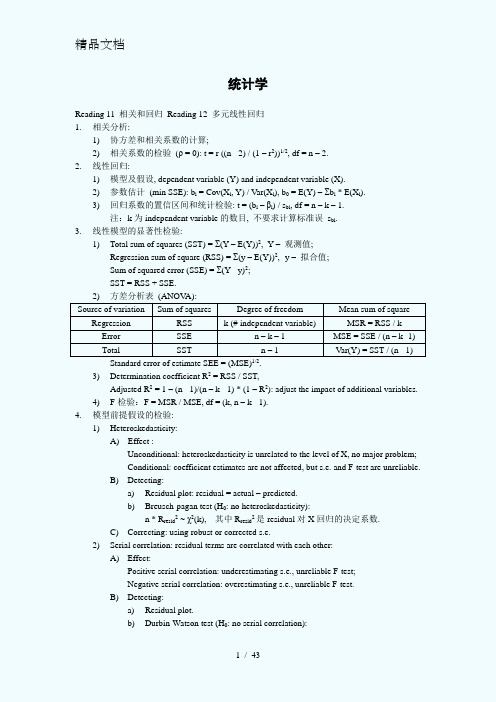
统计学Reading 11 相关和回归Reading 12 多元线性回归1. 相关分析:1) 协方差和相关系数的计算;2) 相关系数的检验(ρ = 0): t = r ((n - 2) / (1 – r2))1/2, df = n – 2.2. 线性回归:1) 模型及假设, dependent variable (Y) and independent variable (X).2) 参数估计(min SSE): b i = Cov(X i, Y) / Var(X i), b0 = E(Y) –Σb i * E(X i).3) 回归系数的置信区间和统计检验: t = (b i–βi) / s bi, df = n – k – 1.注:k为independent variable的数目, 不要求计算标准误s bi.3. 线性模型的显著性检验:1) Total sum of squares (SST) = Σ(Y – E(Y))2, Y –观测值;Regression sum of square (RSS) = Σ(y – E(Y))2, y –拟合值;Sum of squared error (SSE) = Σ(Y - y)2;SST = RSS + SSE.2) 方差分析表(ANOV A):Source of variation Sum of squares Degree of freedom Mean sum of square Regression RSS k (# independent variable) MSR = RSS / k Error SSE n – k – 1 MSE = SSE / (n – k -1) Total SST n – 1 Var(Y) = SST / (n - 1)Standard error of estimate SEE = (MSE)1/2.3) Determination coefficient R2 = RSS / SST,Adjusted R2 = 1 – (n - 1)/(n – k - 1) * (1 – R2): adjust the impact of additional variables.4) F-检验:F = MSR / MSE, df = (k, n – k - 1).4. 模型前提假设的检验:1) Heteroskedasticity:A) Effect :Unconditional: heteroskedasticity is unrelated to the level of X, no major problem;Conditional: coefficient estimates are not affected, but s.e. and F-test are unreliable.B) Detecting:a) Residual plot: residual = actual – predicted.b) Breusch-pagan test (H0: no heteroskedasticity):n * R resid2 ~ χ2(k), 其中R resid2是residual对X回归的决定系数.C) Correcting: using robust or corrected s.e.2) Serial correlation: residual terms are correlated with each other:A) Effect:Positive serial correlation: underestimating s.e., unreliable F-test;Negative serial correlation: overestimating s.e., unreliable F-test.B) Detecting:a) Residual plot.b) Durbin-Watson test (H0: no serial correlation):DW ≈ 2(1 - r), 其中r是残差的自相关系数, 0 ≤ DW ≤ 4.C) Correcting: corrected s.e. for both serial correlation and heteroskedasticity.3) Multicollinearity: independent variables are highly correlated with each other:A) Effect: individual variables are not significant (large s.e.) but their combination is.B) Detecting:a) None of individual coefficient is significant, but F-test is.b) Correlations between variables (> 0.7).注:两变量间的相关系数并未考虑变量线性组合的相关性,因此低相关系数并不一定意味着不存在multicollinearity.C) Correcting: omit correlated variables or take stepwise regression.4) Model misspecification: 不合适地选取解释变量(实际意义不对或不满足线性模型的前提假设)或不恰当的变量转换等.5. Dummy variable (0 – 1 variable):1) Independent dummy variable: linear regression is appropriate.注:n classes → (n - 1) dummy variable.2) Qualitative dependent variable (Y取0, 1): ordinary regression may not be appropriate, use logit regression model or discriminate model.Reading 13 时间序列分析1. Trend model:1) Linear: x t = b0 + b1t + εt;2) Log-linear: ln(x t) = b0 + b1t + εt, 常用于为增长率建模.2. Autoregressive model (AR):1) AR(p): x t = b0 + b1x t-1 + … + b p x t-p + εp, lag: 1, … , p.2) Covariance stationarity:a) Constant and finite E(X t): mean-reverting level for AR(1) E(X t) = b0 / (1 – b1).Random walks (unit root process): x t = b0 + x t-1 + εt不是平稳过程.b) Constant and finite Var(X t);c) Constant and finite Cov(X t, X t-k):对AR平稳序列, 自相关系数Cor(X t, X t-k) = ρk→ 0.3) Forecasting:a) In-sample (within the range of data) and out-sample forecasts.b) Short time series: more stable (no dramatic change);Long-time series: more reliable.c) Predicting power: root mean squared error (RMSE) on the out-sample data.3. AR模型的检验与修正:1) Nonstationarity:a) Detecting: Dickey-Fuller (DF) test or unit root test:For AR(1): x t– x t-1 = b0 + (b1 - 1)x t-1 + εt, H0: b1 = 1, t-test with modified s.e.b) Correcting - differencing:For random walks: 令y t = x t– x t-1, 有y t = b0 + εt.2) Serial correlation (residual terms should not exhibit serial correlation):a) Detecting:H0: Cor(εt, εt-k) = 0 for any lag k; t = Cor(εt, εt-k) / (1 / T) 1/2, df = T – p - 1.注: T – number of effective observations, T = n – p.一般线性回归中的DW检验不适用于AR模型。
- 1、下载文档前请自行甄别文档内容的完整性,平台不提供额外的编辑、内容补充、找答案等附加服务。
- 2、"仅部分预览"的文档,不可在线预览部分如存在完整性等问题,可反馈申请退款(可完整预览的文档不适用该条件!)。
- 3、如文档侵犯您的权益,请联系客服反馈,我们会尽快为您处理(人工客服工作时间:9:00-18:30)。
2.1 Interest Rates and Compounding Frequencies
• Interest rates are closely related to discount factors and are more
similar to the concept of return on an investment ▫ Yet it is more complicated, because it depends on the compounding
Let Z(t,T) be the discount factor between dates t and T. Then
the semi-annually compounded interest rate r2(t,T) can be computed from the formula
2.1.1 Semi-annual Compounding
1.1 Discount Factors across Time
Discount factors give the current value (price) of receiving
$1 at some point in the future
These values are not constant over time. One of the
Z(t,T1) ≥ Z(t,T2) the maturity T. That is given two dates T1 and T2, with T1 < T2, it is always the case that
It is always the case that market participants prefer a $1
1 1 r2 t , T 2 1 2 1 4.43% 1 1 Z t , T 2 0.95713 2
important variables that determines this value is inflation
Inflation is exactly what determines the time value of money,
as it determines how much goods money can buy. The higher the expected inflation, the less appealing it is to receive money in the future compared to today, as this money will be able to buy a lesser amount of goods
Lecture 2: Discount Factors and Interest Rates
Rui Guo Hanqing, RUC Fall 2017
Outline
Discount Factor
Interest Rates The Term Structure of Interest Rates
lower interest rate
2.1.1 Semi-annual Compounding
In semi-annual compounding bondholders receive a coupon
payment twice a year
Example:
Let t = August 10, 2006, and let T = August 10, 2007 (one year later) Consider a year investment of $100 at t with semi-annually compounded
1.1 Discount Factors across Maturities
Z(t,T) records the time value of money between t and T At any given time t, the discount factor is lower, the longer
2 Interest Rates
Interest Rates and Compounding Frequencies
Semi-annual Compounding More Frequent Compounding Continuous Compounding
The Relation between Discount Factors and
called the discount factor.
• The discount factor between two dates, t and T, provides the term
of exchange between a given amount of money at t versus a (certain) amount of money at a later date T: Z(t,T) ▫ On Aug 10, 2006 the Treasury issued 182-day Treasury bills. The issuance market price was $97.47 for $100 of face value ▫ That is, investors were willing to buy for $97.47 a government security that would pay $100 on Feb 8, 2007 ▫ This Treasury bill would not make any other payment between the two dates ▫ Thus, the ratio between purchase price and the payoff, 0.9747 = $97.47/$100, can be considered the market-wide discount factor between the two dates Aug 10, 2006 and Feb 8, 2007 ▫ That is, market participants were willing to exchange 0.9747 dollars on the first date for 1 dollar six months later
Another example:
On March 1, 2001 (time t) the Treasury issued a 52-week
Treasury bill, with maturity date T = Feb 28, 2002 The price of the Treasury bill was $95.713 As we have learned, this price defines a discount factor between the two dates of Z(t,T) = 0.95713 At the same time, it also defines a semi-annually compounded interest rate equal to r2(t,T) = 4.43% In fact, $95.713 × (1 + 4.43% / 2)2 = $100 The semi-annually compounded interest rate can be computed from Z(t,T) = 0.95713 by solving for r2(t,T)
Z (t, T ) =
payoff .at.T
=
(1 + r / 2)
2
From Interest Rate to Discount Factor
The semi-annually compounded interest rate r2(t,T) defines a
payoff at maturity T given by
• For a given interest rate, a higher compounding frequency results
in a higher payoff
• For a given payoff, a higher compounding frequency results in a
sooner than later On Aug 10, 2006 the U.S. government also issued 91-day bills
with a maturity date of Nov 9, 2006. The price was $98.74 for $100 of face value Thus, denoting again t = Aug 10, 2006, now T1 = Nov 9, 2006, and T2 = Feb 8, 2007, we find that the discount factor Z(t,T1) = 0.9874, which is higher than Z(t,T2) = 0.9747
1 Discount Factors
Discount Factors across Maturities
Discount Factors over rs
• The value of what $1 in the future would be in today’s money is
frequency
• The compounding frequency of interest accruals refers to the
number of times within a year in which interests are paid on the invested capital