ANSYSMaxwell涡流场分析案例

合集下载

（完整版）关于Ansoftmaxwell中电机铁耗和涡流损耗计算的说明

（完整版）关于Ansoftmaxwell中电机铁耗和涡流损耗计算的说明考虑到最近很多⼈在问这个问题，因此专门整理出来，供新⼿参考。

先谈⼀下什么情况下需要做铁耗分析。

对常规交流电机（同步或者异步电机），只有定⼦铁⼼才会产⽣铁耗，转⼦铁⼼是没有铁耗的，学过电机的⼈都明⽩的。

因此，只需要对定⼦铁⼼给出B-P曲线（也就是铁损曲线）。

注意，B-P 曲线分为单频和多频两种，能给出多频损耗曲线最好，这样maxwell算得准些。

设置完铁损曲线以后，还要记得在excitations/set core loss，对定⼦铁⼼勾选才⾏。

此时，不需要给定⼦和转⼦铁⼼再施加电导率，这是初学者容易忽视的问题。

后处理中，通过result/create transient reports/core loss查看铁耗随时间变化曲线。

再谈⼀下什么情况下需要做涡流损耗分析。

对永磁电机，永磁体受空间⾼次谐波的影响，会在表⾯产⽣涡流损耗；对实⼼转⼦电机，由于是⼤块导体，因此涡流损耗占绝⼤部分。

以上两种情况需要考虑做涡流损耗分析。

现以永磁电机为例，具体阐述。

对永磁体设置电导率，然后对每个永磁体分别施加零电流激励源，在excitations/set eddy effect，对永磁体勾选。

注意，若只考虑永磁体的涡流损耗，⽽不考虑电机其他部分（定转⼦铁⼼）的涡流损耗，则只需要给永磁体赋予电导率值，其他部件不需要赋电导率，这是初学者容易搞错的地⽅。

简⽽⾔之，只对需要考虑涡流损耗的部件，施加电导率，零电流激励和set eddy effect。

后处理中，通过results/create transient reports/retangular report/solid loss查看涡流损耗随时间变化曲线。

最后，再次强调⼀下，做涡流损耗分析，需要skin depth based refinement ⽹格剖分才⾏。

以上⽅法，适⽤于Ansoft maxwell 13.0.0及以上版本，并适⽤于所有电机种类。

ANSYSMaxwell涡流场分析案例教学内容

ANSYSMaxwell涡流场分析案例教学内容ANSYS Maxwell涡流场分析案例教学内容一、引言ANSYS Maxwell是一款强大的电磁场仿真软件，可以用于分析和优化电磁设备和系统。

其中，涡流场分析是ANSYS Maxwell的重要功能之一。

本文将介绍涡流场分析的基本原理和案例教学内容，帮助读者快速上手并应用于实际工程问题。

二、涡流场分析原理涡流场分析是基于安培定律和法拉第电磁感应定律的原理。

当导体材料中有变化的磁场时，会产生涡流。

涡流产生的原因是磁场的变化导致电场的环路产生感应电动势，从而在导体内部产生电流。

涡流的大小和分布情况与导体材料的电导率、磁场的强度和频率等因素有关。

三、案例教学内容1. 涡流场分析基本操作- 创建新项目：打开ANSYS Maxwell软件，点击“File”菜单，选择“New”，输入项目名称并选择适当的单位。

- 导入几何模型：点击“Geometry”菜单，选择“Import”选项，导入需要分析的几何模型文件。

- 定义材料属性：点击“Materials”菜单，选择“Assign/Edit Material Properties”选项，根据实际情况定义导体材料的电导率等属性。

- 设置边界条件：点击“Boundaries”菜单，选择“Assign/Edit Boundary Conditions”选项，设置边界条件，如电流密度、电压等。

- 运行仿真：点击“Solve”菜单，选择“Analyze All”选项，运行涡流场仿真。

- 结果分析：点击“Results”菜单，选择“Postprocess”选项，查看涡流场分布情况，并进行必要的后处理操作。

2. 涡流场分析案例- 案例1：电感器的涡流损耗分析在电感器中，由于交流电磁场的存在，会产生涡流损耗。

通过对电感器进行涡流场分析，可以评估涡流损耗的大小，并优化电感器的设计。

具体步骤如下：1) 导入电感器的几何模型。

2) 定义电感器材料的电导率。

ansoft Maxwell 涡流分析材料(英文)

Chapter 6.0 Chapter 6.0 –Eddy Current Examples6.1 –Asymmetrical Conductor with a HoleExample (Eddy Current) –Asymmetrical ConductorThe Asymmetrical Conductor with a HoleThis example is intended to show you how to create and analyze anAsymmetrical Conductor with a Hole using the Eddy Current solver in the Ansoft Maxwell 3D Design Environment.Coil (Copper)Stock (Aluminum)Example (Eddy Current) –Asymmetrical Conductor Getting StartedLaunching Ansoft Maxwell1.To access Ansoft Maxwell, click the Microsoft Start button, select Programs, andselect the Ansoft > Maxwell 11program group. Maxwell 11.Setting Tool OptionsTo set the tool options:Note: In order to follow the steps outlined in this example, verify that thefollowing tool options are set:1.Select the menu item Tools > Options > Maxwell Options2.Maxwell Options Window:1.Click the General Options tabUse Wizards for data entry when creating new boundaries: ;CheckedDuplicate boundaries with geometry: ;Checked2.Click the OK button3.Select the menu item Tools > Options > 3D Modeler Options.4.3D Modeler Options Window:1.Click the Operation tabAutomatically cover closed polylines: ;Checked2.Click the Drawing tabEdit property of new primitives: ;Checked3.Click the OK buttonExample (Eddy Current) –Asymmetrical Conductor Opening a New ProjectTo open a new project:In an Ansoft Maxwell window, click the On the Standard toolbar, orselect the menu item File > New.From the Project menu, select Insert Maxwell Design.Set Solution TypeTo set the solution type:Select the menu item Maxwell > Solution TypeSolution Type Window:Choose Eddy CurrentClick the OK buttonExample (Eddy Current) –Asymmetrical Conductor Creating the 3D ModelSet Model UnitsTo set the units:1.Select the menu item 3D Modeler > Units2.Set Model Units:1.Select Units: mm2.Click the OK buttonSet Default MaterialTo set the default material:ing the 3D Modeler Materials toolbar, choose Select2.Select Definition Window:1.Type aluminum in the Search by Name field2.Click the OK buttonExample (Eddy Current) –Asymmetrical Conductor Create StockTo create the stock:1.Select the menu item Draw > Boxing the coordinate entry fields, enter the box positionX: 0.0, Y: 0.0, Z: 0.0, Press the Enter keying the coordinate entry fields, enter the opposite corner of the box:dX: 294.0, dY: 294.0, dZ: 19.0, Press the Enter key To set the name:1.Select the Attribute tab from the Properties window.2.For the Value of Name type: stock3.Click the OK buttonTo fit the view:1.Select the menu item View > Fit All > Active View.Create Hole in StockTo create the hole:1.Select the menu item Draw > Boxing the coordinate entry fields, enter the box positionX: 18.0, Y: 18.0, Z: 0.0, Press the Enter keying the coordinate entry fields, enter the opposite corner of the box:dX: 126.0, dY: 126.0, dZ: 19.0, Press the Enter key To set the name:1.Select the Attribute tab from the Properties window.2.For the Value of Name type: hole3.Click the OK buttonTo select the objects:1.Select the menu item Edit > Select AllTo complete the stock:1.Select the menu item 3D Modeler > Boolean > Subtract2.Subtract WindowBlank Parts: stockTool Parts: holeClick the OK buttonExample (Eddy Current) –Asymmetrical ConductorSet Default Materialing the 3D Modeler Materials toolbar, choose Select2.Select Definition Window:1.Type copper in the Search by Name field2.Click the OK buttonCreate Coil (Hole)To create coil:1.Select the menu item Draw > Boxing the coordinate entry fields, enter the box positionX: 119.0, Y: 25.0, Z: 49.0, Press the Enter keying the coordinate entry fields, enter the opposite corner of the box:dX: 150.0, dY: 150.0, dZ: 100.0, Press the Enter keyTo set the name:1.Select the Attribute tab from the Properties window.2.For the Value of Name type: coil_hole3.Click the OK buttonTo create the filets:1.Select the menu item Edit > Select > Edges.ing the mouse graphically select the 4 z-directed edges. Hold down theCTRL key to make multiple selections.3.Select the menu item 3D Modeler > Fillet4.Fillet Properties1.Fillet Radius: 25mm2.Setback Distance:0mm3.Click the OK buttonSelect 4 EdgesExample (Eddy Current) –Asymmetrical Conductor Create CoilTo create coil:1.Select the menu item Draw > Boxing the coordinate entry fields, enter the box positionX: 94.0, Y: 0.0, Z: 49.0, Press the Enter keying the coordinate entry fields, enter the opposite corner of the box:dX: 200.0, dY: 200.0, dZ: 100.0, Press the Enter key To set the name:1.Select the Attribute tab from the Properties window.2.For the Value of Name type: coil3.Click the OK buttonTo create the filets:1.Select the menu item Edit > Select > Edges.ing the mouse graphically select the 4 z-directed edges. Hold down theCTRL key to make multiple selections.3.Select the menu item 3D Modeler > Fillet4.Fillet Properties1.Fillet Radius: 50mm2.Setback Distance:0mm3.Click the OK buttonTo select the object for subtract1.Select the menu item Edit > Select > Objects2.Select the menu item Edit > Select > By Name3.Select Object Dialog,1.Select the objects named: coil, coil_hole2.Click the OK buttonTo complete the coil:1.Select the menu item 3D Modeler > Boolean > Subtract2.Subtract WindowBlank Parts: coilTool Parts: coil_holeClick the OK buttonTo fit the view:1.Select the menu item View > Fit All > Active View.Example (Eddy Current) –Asymmetrical Conductor Create Offset Coordinate SystemTo create an offset Coordinate System:1.Select the menu item 3D Modeler > Coordinate System > Create >Relative CS > Offseting the coordinate entry fields, enter the originX: 200.0, Y: 100.0, Z: 0.0, Press the Enter keyCreate ExcitationObject Selection1.Select the menu item Edit > Select > By Name2.Select Object Dialog,1.Select the objects named: coil2.Click the OK buttonSection Object1.Select the menu item Edit > Surface > Section1.Section Plane:XZ2.Click the OK buttonSeparate Bodies1.Select the menu item Edit > Boolean > Separate BodiesAssign Excitation1.Select the menu item Maxwell > Excitations > Assign > Current2.Current Excitation : General: Current12.Value: 2742 A3.Type: StrandedNote:The current flow should be counter-clockwise when viewingthe coil from above. Use the Swap Direction button to change thedirection.3.Click the OK buttonExample (Eddy Current) –Asymmetrical ConductorSet Eddy EffectTo set the eddy effect for the stock object1.Select the menu item Maxwell > Excitations > Set Eddy Effects2.Set Eddy Effect,1.Check the settings as shown2.Click the OK buttonShow Conduction PathShow Conduction Path1.Select the menu item Maxwell > Excitations > Conduction Paths > ShowConduction Paths2.From the Conduction Path Visualization dialog, select the rows to visualizethe conduction path in on the 3D Model.3.Click the Close buttonDefine a RegionTo define a Region:1.Select the menu item Draw > Region1.Padding Date:One2.Padding Percentage:3003.Click the OK buttonExample (Eddy Current) –Asymmetrical Conductor Analysis SetupCreating an Analysis SetupTo create an analysis setup:1.Select the menu item Maxwell > Analysis Setup > Add Solution Setup2.Solution Setup Window:1.Click the General tab:Percent Error: 22.Click the Convergence tab:Refinement Per Pass: 50 %3.Click the Solver tab:Adaptive Frequency: 200 Hz4.Click the OK buttonSave ProjectTo save the project:1.In an Ansoft Maxwell window, select the menu item File > Save As.2.From the Save As window, type the Filename: maxwell_asymcond3.Click the Save buttonAnalyzeModel ValidationTo validate the model:1.Select the menu item Maxwell > Validation Check2.Click the Close buttonNote:To view any errors or warning messages, use the MessageManager.AnalyzeTo start the solution process:1.Select the menu item Maxwell > Analyze AllExample (Eddy Current) –Asymmetrical Conductor Create ReportsCreate z-component of B-Field (real part) vs. Distance plot on a line To create a line:1.Make sure that the Global Coordinate System is selected:3D Modeler > Coordinate System > Set Working CS2.Select the menu item Draw > Line3.When the dialog appears asking to create a non-model object, click the Yesbutton.4.Select the menu item Draw > Lineing the coordinate entry fields, enter the vertex point:X: 0.0, Y: 72.0, Z: 34.0, Press the Enter keying the coordinate entry fields, enter the vertex point:X: 288.0, Y: 72.0, Z: 34.0, Press the Enter keying the mouse, right-click and select DoneTo set the name:1.Select the Attribute tab from the Properties window.2.For the Value of Name type: FieldLine3.Click the OK buttonExample (Eddy Current) –Asymmetrical ConductorTo calculate real part of the z-component of B-field (use the fields calculator)1.Select the menu item Maxwell > Fields > Calculator2.Select Quantity:B3.Select Vector: Scal?> Scalar Z4.Select General: Complex > Real5.Click the Smooth button6.Click the Number Button1.Type: Scalar2.Value: 100003.Click the OK button7.Click the *button8.Click the Add buttond Expression:Bz_real2.Click the OK button10.Click the Done buttonCreate Report1.Select the menu item Maxwell > Results > Create Report2.Create Report Window:1.Report Type: Fields2.Display Type: Rectangular3.Click the OK button3.Traces Window:1.Solution: Setup1: LastAdaptive2.Domain: FieldLine3.Click the Y tab1.Category:Calculator Expressions2.Quantity: Bz_real3.Function: <none>4.Click the Add Trace button4.Click the Done buttonExample (Eddy Current) –Asymmetrical ConductorField OverlaysCreate Field OverlayTo select an objectSelect the menu item Edit > Select > By NameSelect Object Dialog,Select the objects named: stockClick the OK buttonTo create a field plot:1.Select the menu item Maxwell > Fields > Fields> J > Mag_J2.Create Field Plot Window1.Solution: Setup1 : LastAdaptive2.Quantity: Mag_J3.In Volume: All4.Plot on Surface Only: ;Checked5.Click the Done buttonExample (Eddy Current) –Asymmetrical Conductor Create Field OverlayTo select an objectSelect the menu item Edit > Select > By NameSelect Object Dialog,Select the objects named: stockClick the OK buttonTo create a field plot:1.Select the menu item Maxwell > Fields > Fields> J > Vector_J2.Create Field Plot Window1.Solution: Setup1 : LastAdaptive2.Quantity: Vector_J3.In Volume: All4.Plot on Surface Only: ;Checked5.Click the Done buttonTo modify a Magnitude field plot:1.Select the menu item Maxwell > Fields > Modify Plot Attributes2.Select Plot Folder Window:1.Select: J2.Click the OK button3.J Window:1.Click the Plots tab1.Plot: Vector_J12.Vector Plot3.Set the Spacing slider to the minimum2.Click the Marker/Arrow tab1.Arrow Options2.Map Size: Unchecked3.Arrow Tail: Uncheckede the slider bar to adjust thesize2.Click the Close button。

Ansoft Maxwell简介与电场仿真实例PPT精选文档

显示横截面电场矢量图
在history tree窗口中选中Plane： Global:XY
在Project manage窗口中
Field Overlays，右键单击
Fields > E > E_Vector
22
9.后处理显示剖分结果图选中模型Inner，Outer 在Project manage窗口中 Field Overlays，右键单击 Fields > Plot Mesh
Grid Output Min: [-0.002 -0.002 0] Max: [0.002 0.002 0.001] Grid Size: [0.0001 0.0001 0.001] Vector data "Domain(Volume(AllObjects), <Ex,Ey,Ez>)“
-2.0000000000000000e-003 -2.0000000000000000e-003 0.0000000000000000e+000
-2.6696090154630286e+002 -3.6309353467063706e+003 -1.9492643644693467e+002
………
场点坐标
电场强度分量 Ex，Ey，Ez
26
18
5.设置自适应求解器收敛判据 Maxwell 3D> Analysis Setup > Add Solution Setup 最大迭代循环次数：10 误差：< 5%
每次迭代加密剖分比例：50%
19
6.检验所有设置是否正确
单击
7.求解
单击
20
8.查看收敛结果 Maxwell 3D> Results > Solution Data

Ansoft Maxwell 仿真实例PDF(68页)

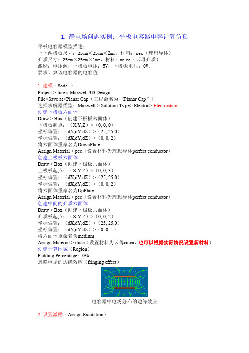
1. 静电场问题实例：平板电容器电容计算仿真平板电容器模型描述：上下两极板尺寸：25mm×25mm×2mm，材料：pec（理想导体）介质尺寸：25mm×25mm×1mm，材料：mica（云母介质）激励：电压源，上极板电压：5V，下极板电压：0V。

要求计算该电容器的电容值1.建模（Model）Project > Insert Maxwell 3D DesignFile>Save as>Planar Cap（工程命名为“Planar Cap”）选择求解器类型：Maxwell > Solution Type> Electric> Electrostatic创建下极板六面体Draw > Box（创建下极板六面体）下极板起点：（X,Y,Z）>（0, 0, 0）坐标偏置：（dX,dY,dZ）>（25, 25,0）坐标偏置：（dX,dY,dZ）>（0, 0, 2）将六面体重命名为DownPlateAssign Material > pec（设置材料为理想导体perfect conductor）创建上极板六面体Draw > Box（创建下极板六面体）上极板起点：（X,Y,Z）>（0, 0, 3）坐标偏置：（dX,dY,dZ）>（25, 25,0）坐标偏置：（dX,dY,dZ）>（0, 0, 2）将六面体重命名为UpPlateAssign Material > pec（设置材料为理想导体perfect conductor）创建中间的介质六面体Draw > Box（创建下极板六面体）介质板起点：（X,Y,Z）>（0, 0, 2）坐标偏置：（dX,dY,dZ）>（25, 25,0）坐标偏置：（dX,dY,dZ）>（0, 0, 1）将六面体重命名为mediumAssign Material > mica（设置材料为云母mica，也可以根据实际情况设置新材料）创建计算区域（Region）Padding Percentage：0%忽略电场的边缘效应（fringing effect）电容器中电场分布的边缘效应2.设置激励（Assign Excitation）选中上极板UpPlate,Maxwell 3D> Excitations > Assign >Voltage > 5V选中下极板DownPlate,Maxwell 3D> Excitations > Assign >Voltage > 0V3.设置计算参数（Assign Executive Parameter）Maxwell 3D > Parameters > Assign > Matrix > Voltage1, Voltage2 4.设置自适应计算参数（Create Analysis Setup）Maxwell 3D > Analysis Setup > Add Solution Setup最大迭代次数：Maximum number of passes > 10 误差要求：Percent Error > 1%每次迭代加密剖分单元比例：Refinement per Pass > 50%5. Check & Run6. 查看结果Maxwell 3D > Reselts > Solution data > Matrix电容值：31.543pF2. 恒定电场问题实例：导体中的电流仿真恒定电场：导体中，以恒定速度运动的电荷产生的电场称为恒定电场，或恒定电流场（DC conduction ）恒定电场的源：（1）Voltage Excitation ，导体不同面上的电压（2）Current Excitations ，施加在导体表面的电流（3）Sink （汇），一种吸收电流的设置，确保每个导体流入的电流等于流出的电流。

基于Maxwell的感应电机涡流场分析实例

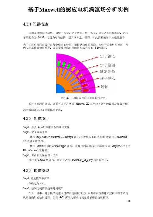
基于Maxwell 的感应电机涡流场分析实例4.3.1 问题描述三相笼型感应电动机，由定子铁心、定子绕组、转子铁心、鼠笼条和转轴组成。

定转子槽配合为子槽配合为 36/32，电机为对称结构，建立四分之一模型。

因此需要施加主从边界条件，，电机为对称结构，建立四分之一模型。

因此需要施加主从边界条件，为了计算电机额定运行过程中输出的转矩，根据感应电机理论，在转子铝条材料设置中考虑实际工作等效电导率。

该鼠笼性感应电机的结构示意图如虑实际工作等效电导率。

该鼠笼性感应电机的结构示意图如 4-60 所示。

所示。

图 4-60 三相鼠笼感应电机结构示意图三相鼠笼感应电机结构示意图通过本问题的分析，读者可以学习掌握通过本问题的分析，读者可以学习掌握 Maxwell 2D 主从边界条件的设置及加载过程，主从边界条件的设置及加载过程，涡流激励源加载及涡流场图处理。

涡流激励源加载及涡流场图处理。

4.3.2 创建项目Step1. 启动启动 Ansoft 并建立新的项目文件并建立新的项目文件 Step2. 定义分析类型定义分析类型执行执行 Project/Insert Maxwell 2D Design命令，或者单击工具栏上按钮建立按钮建立maxwell 2D 设计分析类型。

设计分析类型。

执行执行 Maxwell 2D/Solution Type 命令，在弹出的求解器对话框中选择命令，在弹出的求解器对话框中选择 Magnetic 栏下的栏下的 Eddy Current 求解器。

求解器。

Step3. 重命名及保存项目文件重命名及保存项目文件执行执行 File/Save as 命令，将名称改为命令，将名称改为 Induction_M_eddy 后进行保存。

后进行保存。

4.3.3 构建模型Step1. 确定模型单位单位确定为位确定为mm 。

Step2. 绘制电机槽及绕组几何模型绘制电机槽及绕组几何模型在上一例中，对于模型的建立过程讲述的较细致，本例中在模型建立过程中将忽略电机槽及绕组的绘制过程，如图机槽及绕组的绘制过程，如图 4-61 所示为感应电机定转子槽及绕组模型。

工程电磁场报告——maxwell

=
1
2 H Rs S t 2
= 2δσ =
H2 t
H2 t 2
ωμ 2σ
S
式中，S 为叠片表面积；Ht 为磁场强度切向分量；σ为叠片电导率；μ为叠片相对磁导率；ω为外加磁场角频率；R s 为单位表面积叠片的阻抗；δ为趋肤深度。此公式适用于频率大于 10KHZ 的情况，为了进行对比，也利用此公式计算 2KHZ 和 5KHZ 的情况。高频数值计算结果与实验值的比较 F（Hz） 2k 5k 10k 3 误差分析误差表格 F(Hz) 1 60 360 1K 2K 5K 10K Bmin 0.004% 0.097% 8.11% 16.4% 18.8% 7.91% 0.27% P 3.3% 3.3% 5.5% 17% 42%（低） 20%（高） 80%（低） 34%（低） 6.6%（高） 1.9%（高） Bmin（T） 0.7167 0.3208 0.0666 P（W）[理论] 5.6918 9.0000 12.727 P（W）[实验] 4.64186 9.47030 1.24261e1
高频公式理论表格 F(Hz) 5000 3）误差分析误差表格 F(Hz) 50 200 5000 Bmin 0.03% 0.04% 0.11% P 0.07% 0.13% 47.5%(低) 2.0%(高) Bmin(T) 0.0288 P(W) 1.13868e001
经过对比发现在 50HZ 和 200HZ 时,仿真结果与低频损耗计算结果吻合较好；在 5000HZ 时,仿真结果与高频损耗计算结果吻合也较好。而对于 Bmin 来说，3 个频率时候吻合得都非常好。二、叠钢片的涡流分析不同频率下的 Bmin 和 P F（Hz） 1 60 Bmin（T） 0.9997 0.9993 第8页共8页 P（W） 1.99214e-6 7.16701e-3

基于AnsoftMaxwell3D涡流场的铜排仿真分析

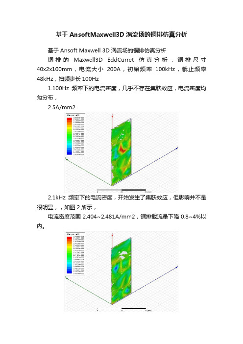
基于AnsoftMaxwell3D涡流场的铜排仿真分析基于Ansoft Maxwell 3D涡流场的铜排仿真分析铜排的Maxwell3D EddCurret仿真分析，铜排尺寸40x2x100mm，电流大小200A，初始频率100kHz，截止频率48kHz，扫频步长100Hz1.100Hz频率下的电流密度，几乎不存在集肤效应，电流密度均匀分布，2.5A/mm22.1kHz频率下的电流密度，开始发生了集肤效应，但影响并不是很明显，，如图2所示，电流密度范围2.404~2.481A/mm2，铜排载流量下降0.8~4%以内。

3. 1.5kHz频率下的电流密度，开始发生了集肤效应增加，但影响并不是很明显，如图2所示，电流密度范围2.32~2.44A/mm2，铜排载流量下降0.4~7.2%以内。

4. 2.5kHz频率下的电流密度，开始发生了集肤效应增加，影响很明显，如图2所示，电流密度范围2.09~2.34A/mm2，铜排载流量下降6.4~16.4%以内。

5.12kHz频率下的电流密度，很明显发生了集肤效应，电流密度均匀分布，如图2所示，电流密度范围0.325~1.07A/mm2，很明显铜排的载流量下降6.24kHz频率下的电流密度，很明显发生了集肤效应，电流密度均匀分布，如图2所示，电流密度范围0.019 ~0.506A/mm2，铜排的载流量进一步下降7.48kHz频率下的电流密度，很明显发生了集肤效应，电流密度均匀分布，如图2所示，电流密度范围0.0078 ~0.173A/mm2，铜排的载流量进一步下降分析与结论在大功率电力电子应用中，不仅仅核心的功率半导体器件需要严格的散热分析和设计，另外，交直流铜排也需要进行一定散热分析和处理，但其要求远远低于功率半导体器件。

A.SVG交流侧铜排：基本上输出的是基波电流，即50Hz的工频电流，另有含量非常低的谐波电流(一般谐波电流畸变率THD<3%)和开关纹波电流(占总电流5%左右)。

1、下载文档前请自行甄别文档内容的完整性，平台不提供额外的编辑、内容补充、找答案等附加服务。
2、"仅部分预览"的文档,不可在线预览部分如存在完整性等问题,可反馈申请退款(可完整预览的文档不适用该条件!)。
3、如文档侵犯您的权益，请联系客服反馈,我们会尽快为您处理(人工客服工作时间：9:00-18:30)。

1.训练后处理应用实例本例中的涡流模型由一个电导率σ=106S/m，长度为100mm，横截面积为10×10m2的导体组成，导体通有幅值为100A、频率为60Hz、初始相位ф=120°的电流。

（一）启动M a x w e l l并建立电磁分析1.在windows系统下执行“开始”→“所有程序”→ANSYS Electromagnetic→ANSYSElectromagnetic Suite 15.0→Windows 64-bit→Maxwell 3D命令，进入Maxwell软件界面。

2.选择菜单栏中File→Save命令，将文件保存名为“training_post”3.选择菜单栏中Maxwell 3D→Solution Type命令，弹出Solution Type对话框(1)Magnetic:eddy current(2)单击OK按钮4.依次单击Modeler→Units选项，弹出Set Model Units对话框，将单位设置成m，并单击OK按钮。

（二）建立模型和设置材料1.依次单击Draw→Box命令，创建长方体在绝对坐标栏中输入：X=-5，Y=-5，Z=0，并按Enter键在相对坐标栏中输入：dX=5，dY=5，dZ=100，并按Enter键单击几何实体，左侧弹出属性对话框，重命名为：Cond材料设置为conductor，电导率为σ=106S/m2.依次单击Draw→Box命令，创建长方体在绝对坐标栏中输入：X=55，Y=-10，Z=40，并按Enter键在相对坐标栏中输入：dX=75，dY=10，dZ=60，并按Enter键单击几何实体，左侧弹出属性对话框，重命名为：aux3.依次单击Draw→Line在绝对坐标栏中输入：X=0，Y=0，Z=0，并按Enter键在相对坐标栏中输入：dX=0，dY=0，dZ=100，并按Enter键名为line14.依次单击Draw→line，生成长方形对角点为（20，-20，50）、（-20，20，50），名为line25.依次单击Draw→Region命令，弹出Region对话框，设置如下:Pad individual directions（-100，-100，0）、（200，100，100）（三）指定边界条件和源1.按f键，选择Cond与Region的交界面，依次单击菜单中的Maxwell 3D→Excitations→Assign→Current命令，在对话框中填入以下内容：(1)Name:SourceIn(2)Value:100 A(3)Palse:120deg(4)单击OK按钮2.按f键，选择Cond与Region的另一个交界面，依次单击菜单中的Maxwell 3D→Excitations→Assign→Current命令，在对话框中填入以下内容：(5)Name:SourceIn(6)Value:100 A(7) Palse:120deg(8) 按Swap Direction 和OK 按钮（四）设置求解规则1. 依次选择菜单栏中Maxwell 3D →Analysis Setup →Add Solution Setup 命令，此时弹出Solution Setup 对话框，在对话框中设置：(1) Maximum number of passes （最大迭代次数）：10(2) Percent Error （误差要求）:1%(3) Refinement per Pass （每次迭代加密剖分单元比例）:50%(4) Solver>Adaptive Frequency （设置激励源的频率）:60Hz(5) 单击OK 按钮。

1. 依次选择菜单栏中的Maxwell 3D→Validation Check 命令，此时弹出的对话框中，如果全部项目都有说明前处理操作没有问题；如果有弹出，则需要重新检查模型；如果有！出现，则不会影响计算。

2. 依次选择Maxwell 3D→Analyze All 命令，此时程序开始计算。

（五）后处理依次单击Maxwell 3D>Fields>Calculator 命令，弹出Fields Calculator 对话框1) 导体内的功率损耗（体积分）方法一：1．选择Input>Quantity>Ohmic Loss2．选择Input>Geometry 选择V olume ，在列表中选择Cond ，然后单击OK 按钮3．选择Scalar>∫Integrate4．选择Output>Eval5．得到Cond 计算损耗约为5方法二：计算公式为dV J J P CondCond ⎪⎪⎭⎫ ⎝⎛⋅=⎰σ*Re 21 1．选择Input>Quantity>J ，获得电流密度矢量J ；2．选择Push3．选择General>Complex ：Conj ，求J 的共轭；4．选择Vector>Mtal ，出现Material Operation 窗口；5．选择Conductivity 、Divide ；单击OK 按钮6．选择Vector>Dot7．选择General>Complex ：Real ；8．选择Input>Number ，设置为Type:Scalar ；Value:2；单击OK9．选择General>/10．选择Input>Geometry 选择V olume ，在列表中选择Cond ，然后单击OK 按钮11．选择Scalar>∫Integrate12．选择Output>Eval13．得到Cond 计算损耗约为52) 沿着导体路径的电压降（线积分）计算电压降的实部：计算公式为dl J U line R ⋅⎥⎦⎤⎢⎣⎡=⎰1Re σ 1．选择Input>Quantity>J ，获得电流密度矢量J ；2．选择Vector>Mtal ，出现Material Operation 窗口；3．选择Conductivity 、Divide ；单击OK 按钮4．选择General>Complex ：Real ；5．选择Input>Geometry 选择Line ，在列表中选择Line1，然后单击OK 按钮6．选择Vector>Tangent7．选择Scalar>∫Integrate8．选择Output>Eval9．得到电压降的实部分量为0.05V计算电压降的虚部：计算公式为dl J U line I ⋅⎥⎦⎤⎢⎣⎡=⎰1Im σ 1．选择Input>Quantity>J ，获得电流密度矢量J ；2．选择Vector>Mtal ，出现Material Operation 窗口；3．选择Conductivity 、Divide ；单击OK 按钮4．选择General>Complex ：Imag ；5．选择Input>Geometry 选择Line ，在列表中选择Line1，然后单击OK 按钮6．选择Vector>Tangent7．选择Scalar>∫Integrate8．选择Output>Eval9．得到电压降的实部分量为-0.0866V理论计算电压降幅值为V U U U I R 1.022=+= 3) 安培定律（线积分）计算磁场强度的实部分量沿着线l i n e 2的线积分1．选择Input>Quantity>H ；2．选择General>Complex ：Real ；3．选择Input>Geometry 选择Line ，在列表中选择Line2，然后单击OK 按钮4．选择Vector>Tangent5．选择Scalar>∫Integrate6．选择Output>Eval7．出现86.58A实际电流的实部是100×sin120=86.58A计算磁场强度的虚部分量沿着线l i n e2的线积分1．选择Input>Quantity>H；2．选择General>Complex：Imag；3．选择Input>Geometry选择Line，在列表中选择Line2，然后单击OK按钮4．选择Vector>Tangent5．选择Scalar>∫Integrate6．选择Output>Eval7．出现-49.98A实际电流的虚部是100×cos120=50A计算相位1．选择Exch和Rlup操作，确认计算器顶部为-49.98A，接下来是86.58A 2．选择Trig|Atan2，得到相位为120.0004)计算磁通密度散度（体积分）计算磁通密度的实部分量散度在a u x上的体积分1．选择Input>Quantity>B；2．选择General>Complex：Real；3．选择Vector>Divg4．选择Input>Geometry选择V olume，在列表中选择aux，然后单击OK按钮5．选择Scalar>∫Integrate6．选择Output>Eval7．出现-9.68×10-10A计算磁通密度的虚部分量散度在a u x上的体积分1．选择Input>Quantity>B；2．选择General>Complex：Imag；3．选择Vector>Divg4．选择Input>Geometry选择V olume，在列表中选择aux，然后单击OK按钮5．选择Scalar>∫Integrate6．选择Output>Eval7．出现1.68×10-9A5)磁通量的计算（面积分）磁通量实部的计算1．选择Input>Quantity>B2．选择Vector:Scal?>Scalar Y3．选择General>Complex：Real；4．选择Input>Geometry选择V olume，在列表中选择aux，然后单击OK按钮5．General>Domain6．选择Input>Geometry选择Surface，在列表中选择XZ，然后单击OK按钮7．选择Scalar>∫Integrate8．选择Output>Eval9．出现5.06×10-8Wb磁通量实部的计算1．选择Input>Quantity>B2．选择Vector:Scal?>Scalar Y3．选择General>Complex ：Imag ；4．选择Input>Geometry 选择V olume ，在列表中选择aux ，然后单击OK 按钮5．General>Domain6．选择Input>Geometry 选择Surface ，在列表中选择XZ ，然后单击OK 按钮7．选择Scalar >∫Integrate8．选择Output>Eval9．出现-8.76×10-8Wb磁通量的幅度为1.01×10-7Wb ，进而可以获得导体与积分表面边界构成的矩形环之间的互感为H I L mag mutual 91001.1-⨯==φ在环内感应电压的幅度为 V I fL V mutual induced 51081.32-⨯==π6) 计算总电阻损耗（体积分）----M a x w e l l _v 16_3D _W S 02_B a s i c E d d y C u r r e n t A n a l y s i s1．选择Input>Quantity>Ohmic Loss2．选择Input>Geometry 选择V olume ，在列表中选择Disk ，然后单击OK 按钮3．选择Scalar>∫Integrate4．选择Output>Eval5．得到Disk 计算损耗约为270.38W7) 计算磁通量----06_1_m a x w e l l _e d d y c u r r e n t _A s y m m e t r i c _C o n d u c t o rB z _r e a l1．选择Input>Quantity>B2．选择Vector:Scal?>Scalar Z3．选择General>Complex ：Real ；4．选择General>Smooth注意:在特斯拉(Tesla)的单位中，流量密度将默认显示。