3自控第三章作业
自动控制原理第三章课后习题答案

3-1(1) )(2)(2.0t r t c= (2) )()()(24.0)(04.0t r t c t c t c=++ 试求系统闭环传递函数Φ(s),以及系统的单位脉冲响应g(t)和单位阶跃响应c(t)。
已知全部初始条件为零。
解:(1) 因为)(2)(2.0s R s sC =闭环传递函数ss R s C s 10)()()(==Φ 单位脉冲响应:s s C /10)(= 010)(≥=t t g单位阶跃响应c(t) 2/10)(s s C = 010)(≥=t t t c(2))()()124.004.0(2s R s C s s =++ 124.004.0)()(2++=s s s R s C 闭环传递函数124.004.01)()()(2++==s s s R s C s φ 单位脉冲响应:124.004.01)(2++=s s s C t e t g t 4sin 325)(3-= 单位阶跃响应h(t) 16)3(61]16)3[(25)(22+++-=++=s s s s s s Ct e t e t c t t 4sin 434cos 1)(33----=3-2 温度计的传递函数为11+Ts ,用其测量容器内的水温,1min 才能显示出该温度的98%的数值。
若加热容器使水温按10ºC/min 的速度匀速上升,问温度计的稳态指示误差有多大?解法一 依题意,温度计闭环传递函数11)(+=ΦTs s 由一阶系统阶跃响应特性可知:o o T c 98)4(=,因此有 min 14=T ,得出 min 25.0=T 。
视温度计为单位反馈系统,则开环传递函数为Ts s s s G 1)(1)()(=Φ-Φ= ⎩⎨⎧==11v T K用静态误差系数法,当t t r ⋅=10)( 时,C T Ke ss ︒===5.21010。
解法二 依题意,系统误差定义为 )()()(t c t r t e -=,应有 1111)()(1)()()(+=+-=-==ΦTs TsTs s R s C s R s E s e C T s Ts Ts ss R s s e s e s ss ︒==⋅+=Φ=→→5.210101lim )()(lim 23-3 已知二阶系统的单位阶跃响应为)1.536.1sin(5.1210)(2.1o tt et c +-=-试求系统的超调量σ%、峰值时间tp 和调节时间ts 。
自动控制原理 第三章答案
3-1 解 该线圈的微分方程为 u =+diiR L dt对上式两边取拉氏变换,并令初始条件为零,可得传递函数为()1=()(+)+1I s RU s L R 时间常数+0.005T L R s ==,过渡时间=30.015s t T s =。
3-2 解 如图2-3-2所示系统的闭环传递函数为010()=(s)0.2+1+10+1H K C s KR S K Ts =其中0101+10H K K K =,0.21+10HT K =原系统的时间常数为0.2s ,放大系数为10,为了满足题目的要求,令0.02T s =和10K =,有0.9H K =和010K =。
3-3 解 设为温度计的输入,表示实际水温,设为温度计的输出,表示温度计的指示值,若实际水温为R (常值),则输入为幅值为R 的阶跃函数,输出为(t)=R(1-e )T c τ根据所给条件,有则时间常数。
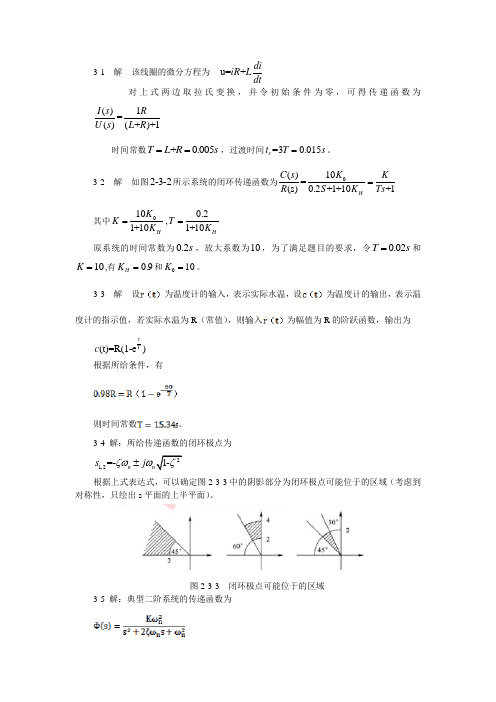
3-4 解:所给传递函数的闭环极点为21,2=-1-n n s j ζωωζ±根据上式表达式,可以确定图2-3-3中的阴影部分为闭环极点可能位于的区域(考虑到对称性,只绘出s 平面的上半平面)。
图2-3-3 闭环极点可能位于的区域3-5解:典型二阶系统的传递函数为由如图2-3-4所示的响应曲线,可知峰值时间,超调量,根据二阶系统的性能指标计算公式和可以确定和,根据如图2-3-4所示曲线的终值,可以确定。
3-6 解:如图2-3-5所示系统的传递函数为是一个典型的二阶系统,其自然振荡频率为,令阻尼比可以确定,性能指标及分别为3-7 解:系统为典型二阶系统,自然振荡频率,阻尼比。
单位阶跃响应的表达式为(t>0)单位斜坡响应的表达式为3-8 解:当时,系统的闭环传递函数为其中,无阻尼自然振荡频率,阻尼比,单位阶跃响应的超调量峰值时间和过度过程时间分别为16.3%、0,36s和0.7s当,时系统的闭环传递函数为其中,无阻尼自然振荡频率,阻尼比,单位阶跃响应的超调量、峰值时间和过渡过程时间分别为30.9%、0.24s和0.7s。
自控及应用第三章习题

τ s
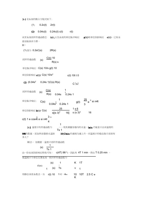
s3 1 10 s2 (1+10 ) 10 τ b31 s1 s0 10 τ >0
第三章习题课 (3-14)
3-14 已知系统结构如图,试确定系统稳 定时τ值范围。
R(s)
解: 10( s+1) τ G(s)= s2(s+1) s3 s2 s1 s0 1 1 b31 10 τ 10 10
第三章习题课 (3-1)
3-1 设温度计需要在一分钟内指示出响应值 的98%,并且假设温度计为一阶系统,求时 间常数T。如果将温度计放在澡盆内,澡盆 的温度以10oC/min的速度线性变化,求温度 计的误差。 解: c(t)=c(∞)98% t=4T=1 min T=0.25 -t/T c(t)=10(t-T+e ) r(t)=10t e(t)=r(t)-c(t) =10(T- e-t/T) ess=lim e(t) =10T=2.5 t→∞
R(s)
-
-
C(s) K s(0.5s+1) τ s
第三章习题课 (3-11)
3-11 已知闭环系统的特征方程式,试用 劳斯判据判断系统的稳定性。 (3) s4+8s3+18s2+16s+5=0 解: 劳斯表如下: (1) s3+20s2+9s+100=0 s4 1 18 5 劳斯表如下: s3 8 16 s3 1 9 s2 16 5 s2 20 100 1 216 s 16 s1 4 s0 100 系统稳定。 s0 5 系统稳定。
R(s)= s1 3
第三章习题课 (3-18)
3-18 已知系统结构如图。为使ζ=0.7时 单位斜坡输入的稳态误差ess=0.25 确定 K 和 τ值 。 R(s) K C(s) - s(s+2) K 解: G(s)= s2+2s+K s τ K Φ(s)= s2+(2+K )s+K τ τ ess= 2+K =0.25 τ ζ 2 ω n=2+K =2*0.7 K K ω n2 =K τ = 0.25K-2 K =31.6 τ =0.186 K K 2+K τ = 1 s+1) s(2+K τ
自动控制原理第三章课后习题答案(最新)汇总
3-1设系统的微分方程式如下:(1)0.2c(t) 2r(t)单位脉冲响应:C(s) 10/s g(t) 103t3 3tc(t) 1 e cos4t e si n4t413-2 温度计的传递函数为 —,用其测量容器内的水温,1min 才能显示出该温度的Ts 198%的数值。
若加热容器使水温按 10(C/min 的速度匀速上升,问温度计的稳态指示误差有多大?解法一 依题意,温度计闭环传递函数由一阶系统阶跃响应特性可知: c(4T) 98 o o ,因此有 4T 1 min ,得出T 0.25 min 。
视温度计为单位反馈系统,则开环传递函数为(s)1K 1TG(s)—1(s) Tsv 1用静态误差系数法,当r(t) 10t 时,e ss10 10T 2.5 C oK(2) 0.04c(t)0.24c(t) c(t)r(t)试求系统闭环传递函数① 部初始条件为零。
解:(s),以及系统的单位脉冲响应 g(t)和单位阶跃响应 c(t)。
已知全(1)因为 0.2sC(s)2R(s) 闭环传递函数(s)C(s) 10R(s) s单位阶跃响应c(t) C(s) 10/s 2c(t) 10t t 0(2) (0.04s 20.24s 1)C(s) R(s)C (s )闭环传递函数(s)C(s) R(s)120.04s0.24s 1单位脉冲响应:C(s)120.04s 2 0.24s 1g(t)25 e 33tsi n4t单位阶跃响应h(t) C(s)25 s[(s 3)216]1 s 6 s (s 3)216(s)1 Ts 1解法二依题意,系统误差疋义为e(t) r(t) c(t),应有e(s)E(s)1 C(s)R(s)11 TsR(s) Ts 1 Ts 13-3 已知二阶系统的单位阶跃响应为c(t) 10 12.5e 1.2t sin(1.6t 53.1o)试求系统的超调量c%、峰值时间t p和调节时间t'si n( 1n t )t p Jl- 1.96(s■1 2n1.63.5 3.5t s 2.92(s)n 1.2或:先根据c(t)求出系统传函,再得到特征参数,带入公式求解指标。
自控第三章答案

K
p
不稳定
稳定
0
K
d
不稳定
不稳定
临界阻尼轨迹: D ( s ) s 4 K d s 4 K
2 p
0 出现重根时
p
临界阻尼条件为: 即: K
2 d
4 K
2
2 d
4 4K
0 线。
K p , 以纵轴为对称轴的抛物 K K
2 d 2 d
过阻尼区: 欠阻尼区: K
B3.15 分析图B3.15所示的两个系统,引入与不引入反馈时 系统的稳定性 。
解 不引入反馈 显然不稳定。 引入反馈 D ( s ) s ( s 1 )( s 5 ) 10 ( s 1 ) 0 闭环稳定。 (s ) 10 ( s 1 ) s ( s 1 )( s 5 )
3
赫尔维茨判据: 9 100 D2 20 1 100 9 80 0
1 20 4 100
2
1
0
故系统是稳定的。
(3)s4+4s3+13s2+36s+K=0
解
(1 ) 劳思判据: s s s s s
4
1 4 4 36 K K
13 36 K K
K 0
3
2
1
0
若系统稳定,则
36 K 0 0 K 36 K 0
( 2 )由
G (s )
7(s 1) s ( s 4 )( s 2 s 2 )
2
0 . 875 ( s 1 ) s ( 0 . 25 s 1 )( 0 . 5 s s 1 )
2
可知系统为
1
型的,于是
自动控制原理第3章练习题

第三章 线性系统的时域分析习题及答案3-1 已知系统脉冲响应t e t k 25.10125.0)(-=试求系统闭环传递函数)(s Φ。
解: Φ()()./(.)s L k t s ==+001251253-2 设某高阶系统可用下列一阶微分方程T c t c t r t r t ∙∙+=+()()()()τ近似描述,其中,1)(0<-<τT 。
试证系统的动态性能指标为t T r =22.T T T t s ⎥⎦⎤⎢⎣⎡-+=)ln(3τ 解: 设单位阶跃输入ss R 1)(=当初始条件为0时有:11)()(++=Ts s s R s C τ 11111)(+--=⋅++=∴Ts T s s Ts s s C ττC t h t T Te t T()()/==---1τ 1) 求t r (即)(t c 从1.0到9.0所需时间)当 Tt e TT t h /219.0)(---==τ; t T T T 201=--[ln()ln .]τ 当 Tt e TT t h /111.0)(---==τ; t T T T 109=--[ln()ln .]τ 则 t t t T T r =-==21090122ln ...2) 求 t sTt s s e TT t h /195.0)(---==τ ]ln 3[]20ln [ln ]05.0ln [lnTT T T T T T T T t s τττ-+=+-=--=∴3-3 一阶系统结构图如图3-45所示。
要求系统闭环增益2=ΦK ,调节时间4.0≤s t s ,试确定参数21,K K 的值。
解: 由结构图写出闭环系统传递函数111)(212211211+=+=+=ΦK K sK K K s K s K K s K s令闭环增益212==ΦK K , 得:5.02=K 令调节时间4.03321≤==K K T t s ,得:151≥K 。
3-4在许多化学过程中,反应槽内的温度要保持恒定, 图3-46(a )和(b )分别为开环和闭环温度控制系统结构图,两种系统正常的K 值为1。
自动控制原理第3章 习题及解析

自动控制原理(上)习 题3-1 设系统的结构如图3-51所示,试分析参数b 对单位阶跃响应过渡过程的影响。
考察一阶系统未知参数对系统动态响应的影响。
解 由系统的方框图可得系统闭环响应传递函数为/(1)()()111K Ts Ks Kbs T Kb s Ts +Φ==++++ 根据输入信号写出输出函数表达式:111()()()()()11/()K Y s s R s K s T Kb s s s T bK =Φ⋅=⋅=-++++对上式进行拉式反变换有1()(1)t T bKy t K e-+=-当0b >时,系统响应速度变慢;当/0T K b -<<时,系统响应速度变快。
3-2 设用11Ts +描述温度计特性。
现用温度计测量盛在容器内的水温,发现1min 可指示96%的实际水温值。
如果容器水温以0.1/min C ︒的速度呈线性变化,试计算温度计的稳态指示误差。
考察一阶系统的稳态性能分析(I 型系统的,斜坡响应稳态误差)解 由开环传递函数推导出闭环传递函数,进一步得到时间响应函数为:()1t T r y t T e -⎛⎫=- ⎪⎝⎭其中r T 为假设的实际水温,由题意得到:600.961Te-=-推出18.64T =,此时求输入为()0.1r t t =⋅时的稳态误差。
由一阶系统时间响应分析可知,单位斜坡响应的稳态误差为T ,所以稳态指示误差为:lim ()0.1 1.864t e t T →∞==3-3 已知一阶系统的传递函数()10/(0.21)G s s =+今欲采用图3-52所示负反馈的办法将过渡过程时间s t 减小为原来的1/10,并保证总的放大倍数不变,试选择H K 和0K 的值。
解 一阶系统的调节时间s t 与时间常数成正比,则根据要求可知总的传递函数为10()(0.2/101)s s Φ=+由图可知系统的闭环传递函数为000(10()()1()0.211010110()0.21110H HHHK G s K Y s R s K G s s K K K s s K ==++++==Φ++)比较系数有101011011010HHK K K ⎧=⎪+⎨⎪+=⎩ 解得00.9,10H K K ==3-4 已知二阶系统的单位阶跃响应为1.5()1012sin(1.6+53.1t y t e t -=-)试求系统的超调量%σ,峰值时间p t ,上升时间r t 和调节时间s t 。
自控第三章作业答案

P3.4 The open-loop transfer function of a unity negative feedback system is)1(1)(+=s s s GDetermine the rise time, peak time, percent overshoot and setting time (using a 5% setting criterion).Solution: Writing he closed-loop transfer function 2222211)(nn ns s s s s ωςωωΦ++=++=we get 1=n ω, 5.0=ς. Since this is an underdamped second-order system with 5.0=ς, thesystem performance can be estimated as follows.Rising time.sec 42.25.0115.0arccos 1arccos 22≈-⋅-=--=πςωςπn r tPeak time.sec 62.35.011122≈-⋅=-=πςωπn p tPercent overshoot %3.16% 100% 100225.015.01≈⨯=⨯=--πςπςσee pSetting time.sec 615.033=⨯=≈ns t ςω(using a 5% setting criterion)P3.5 A second-order system gives a unit step response shown in Fig. P3.5. Find the open-loop transfer function if the system is a unit negative-feedback system.Solution: By inspection we have %30% 100113.1=⨯-=pσSolving the formula for calculating the overshoot,3.021==-ςπςσep, we have362.0ln ln 22≈+-=pp σπσςSince .sec 1=p t , solving the formula for calculating the peak time, 21ςωπ-=n p t , we gets e c / 7.33rad n =ωHence, the open-loop transfer function is )4.24(7.1135)2()(2+=+=s s s s s G n nςωωP3.6 A feedback system is shown in Fig. P3.6(a), and its unit step response curve is shown in Fig. P3.6(b). Determine the values of 1k , 2k , and a ..1.1Figure P3.5Solution: The transfer function between the input and output is given by2221)()(k as sk k s R s C ++=The system is stable and we have, from the response curve,21lim )(lim 122210==⋅++⋅=→∞→k sk as sk k s t c s tBy inspection we have %9% 10000.211.218.2=⨯-=pσSolving the formula for calculating the overshoot, 09.021==-ςπςσep, we have608.0ln ln 22≈+-=pp σπσςSince .sec 8.0=p t , solving the formula for calculating the peak time,21ςωπ-=n p t , we gets e c / 95.4rad n =ωThen, comparing the characteristic polynomial of the system with its standard form, we have22222n n s s k as s ωςω++=++5.2495.4222===n k ω02.695.4608.022=⨯⨯==n a ςωP3.8 For the servomechanism system shown in Fig. P3.8, determine the values of k and a that satisfy the following closed-loop system design requirements. (a) Maximum of 40% overshoot. (b) Peak time of 4s.Solution: For the closed-loop transfer function we have 22222)(nn ns sks k sk s ωςωωαΦ++=++=hence, by inspection, we getk n=2ω, αςωk n =2, and nnkωςςωα22==Taking consideration of %40% 10021=⨯=-ςπςσepresults in280.0=ς.In this case, to satisfy the requirement of peak time, 412=-=ςωπn p t , we have.s e c / 818.0r a d n =ω.2.2(a)(b)Figure P3.6Figure P3.8Hence, the values ofkandaare determined as67.02==n k ω, 68.02==nωςαP3.10 A control system is represented by the transfer function)13.04.0)(56.2(33.0)()(2+++=s ss s R s CEstimate the peak time, percent overshoot, and setting time (%5=∆), using the dominant polemethod, if it is possible.Solution: Rewriting the transfer function as]3.0)2.0)[(56.2(33.0)()(22+++=s s s R s Cwe get the poles of the system: 3.02.02 1j s ±-=,, 56.23-=s . Then, 2 1,s can be considered as a pair of dominant poles, because )Re()Re(32 1s s <<,.Method 1. After reducing to a second-order system, the transfer function becomes13.04.013.0)()(2++=s ss R s C (Note:1)()(lim==→s R s C k s Φ)which results in sec / 36.0rad n =ω and 55.0=ς. The specifications can be determined ass e c 0.42112ςωπ-=n p t , %6.12% 10021=⨯=-ςπςσeps e c 67.2011ln 12=⎪⎪⎪⎭⎫⎝⎛-=ς∆ςωns t Method 2. Taking consideration of the effect of non-dominant pole on the transient components cause by the dominant poles, we haves e c 0.8411)(231=--∠-=ςωπn p s s t%6.13% 10021313=⨯-=-ςπςσes s s ps e c 6.232ln 1313=⎪⎪⎭⎫⎝⎛-⋅=ss s t ns ∆ςωP3.13 The characteristic equations for certain systems are given below. In each case, determine the value of k so that the corresponding system is stable. It is assumed that k is positive number.(a) 02102234=++++k s s s s (b) 0504)5.0(23=++++ks s k sSolution: (a) 02102234=++++k s s s s .The system is stable if and only if⎪⎪⎩⎪⎪⎨⎧<⇒>=>9 022010102203k k D ki.e. the system is stable when 90<<k .(b) 0504)5.0(23=++++ks s k s . The system is stable if and only if⎪⎩⎪⎨⎧>-+⇒>-+⇒>+=>>+0)3.3)(8.34( 05024 041505.00 ,05.022k k k k k k D k ki.e. the system is stable when 3.3>k .P3.14 The open-loop transfer function of a negative feedback system is given by)12.001.0()(2++=s ss Ks G ςDetermine the range of K and ς in which the closed-loop system is stable. Solution: The characteristic equation is02.001.023=+++K s s s ς The system is stable if and only if⎪⎩⎪⎨⎧<⇒>-⇒>=>>ςςς20 001020 0101.02.002.0 ,02K K .ς.K D kThe required range is20>>K ς.P3.17 A unity negative feedback system has an open-loop transfer function )16)(13()(++=s s s K s GDetermine the range ofkrequired so that there are no closed-loop poles to the right of the line1-=s . Solution: The closed-loop characteristic equation is18)6)(3( 0)16)(13(=+++⇒=+++K s s s K s s si.e. 01818923=+++K s s sLetting 1~-=s s resulting in 0)1018(~3~6~ 018)5~)(2~)(1~(23=-+++⇒=+++-K s s s K s s sUsing Lienard-Chipart criterion, all closed-loop poles locate in the right-half s~-plane, i.e. to theright of the line 1-=s , if and only if⎪⎩⎪⎨⎧<⇒>-⇒>-=>⇒>-14 08.182 0311018695 ,010182K K K D K KThe required range is 91495 <<K , or56.10.56 <<KP3.18 A system has the characteristic equation0291023=+++k s s sDetermine the value of k so that the real part of complex roots is 2-, using the algebraic criterion.Solution: Substituting 2~-=s s into the characteristic equation yields 02~292~102~ 23=+-+-+-k s s s )()()( 0)26(~~4~ 23=-+++k s s sThe Routh array is established as shown.If there is a pair of complex roots with real part of 2-, then026=-ki.e. 30=k . In the case of 30=k , we have the solution of the auxiliary equation j s ±=~, i.e. j s ±-=2.3s 1 12s 4 26-k1s 0sP3.22 The open-loop transfer function of a unity negative feedback system is given by)1)(1()(21++=s T s T s Ks GDetermine the values of K , 1T , and 2T so that the steady-state error for the input, bt a t r +=)(, is less than 0ε. It is assumed that K , 1T , and 2T are positive, a and b are constants. Solution: The characteristic polynomial is K s s T T s T T s ++++=221321)()(∆Using L-C criterion, the system is stable if and only if2121212121212 0 01T T T T K T KT T T T T K T T D +<⇒>-+⇒>+=Considering that this is a 1-type system with a open-loop gain K , in the case of 2121T T T T K +<,we have 00.. εεεεεbK Kb v ss r ss ss>⇒<=+=Hence, the required range for K is21210T T T T K b+<<εP3.24 The block diagram of a control system is shown in Fig. P3.24, where )()()(s C s R s E -=. Select the values of τ and b so that the steady-state error for a ramp input is zero.Solution: Assuming that all parameters are positive, the system must be stable. Then, the error response is)()1)(1()(1)()()(21s R K s T s T b s K s C s R s E ⎥⎦⎤⎢⎣⎡++++-=-=τ)()1)(1()1()(2121221s R Ks T s T Kb s K T T sT T ⋅+++-+-++=τLetting the steady-state error for a ramp input to be zero, we get 221212210.)1)(1()1()(lim )(lim sv K s T s T Kb s K T T sT T s s sE s s r ss ⋅+++-+-++⋅==→→τεwhich results in ⎩⎨⎧=-+=-0121τK T T Kb I.e. KT T 21+=τ,Kb 1=.P3.26 The block diagram of a system is shown in Fig. P3.26. In each case, determine the steady-state error for a unit step disturbance and a unit ramp disturbance, respectively. (a) 11)(K s G =,)1()(222+=s T s K s GFigure P3.24Figure P3.26(b)ss T K s G )1()(111+=,)1()(222+=s T s K s G , 21T T >Solution: (a) In this case the system is of second-order and must be stable. The transfer function from disturbance to error is given by 212212.)1(1)(K K Ts s K G G G s d e ++-=+-=ΦThe corresponding steady-state errors are 1212.11)1(lim K s K K Ts s K s s p ss -=⋅++-⋅=→ε∞→⋅++-⋅=→2212.1)1(lim sK K Ts s K s s ass ε(b) Now, the transfer function from disturbance to error is given by )1()1()(121222.+++-=s T K K s T s sK s d e Φand the characteristic polynomial is21121232)(K K s T K K s s T s +++=∆ Using L-C criterion,0)(121211212212>-==T T K K T K K T K K Dthe system is stable. The corresponding steady-state errors are 01)1()1(lim 1212220.=⋅+++-⋅=→ss T K K s T s sK s s p ss ε121212220.11)1()1(lim K ss T K K s T s sK s s a ss -=⋅+++-⋅=→ε。
- 1、下载文档前请自行甄别文档内容的完整性,平台不提供额外的编辑、内容补充、找答案等附加服务。
- 2、"仅部分预览"的文档,不可在线预览部分如存在完整性等问题,可反馈申请退款(可完整预览的文档不适用该条件!)。
- 3、如文档侵犯您的权益,请联系客服反馈,我们会尽快为您处理(人工客服工作时间:9:00-18:30)。
第三章 线性控制系统的能控性和能观性
注明:*为选做题
3-1 判别下列系统的能控性与能观性。
系统中a,b,c,d 的取值对能控性与能观性是否有关,若有关其取值条件如何?
(1)系统如图所示。
题3-1(1)图 系统模拟结构图
(2)系统如图所示。
题3-1(2)图 系统模拟结构图
(3)系统如下式:
1122331122311021010000200000x x x a u x x b x x y c d x y x ∙∙∙⎛⎫-⎛⎫⎛⎫⎛⎫ ⎪ ⎪⎪ ⎪ ⎪=-+ ⎪⎪ ⎪ ⎪ ⎪⎪ ⎪ ⎪-⎝⎭⎝⎭⎝⎭ ⎪⎝⎭
⎛⎫⎛⎫⎛⎫ ⎪= ⎪ ⎪ ⎪⎝⎭⎝⎭ ⎪⎝⎭
3-2 时不变系统:
311113111111x x u y x ∙
-⎛⎫⎛⎫=+ ⎪ ⎪-⎝⎭⎝⎭⎛⎫= ⎪-⎝⎭
试用两种方法判别其能控性与能观性。
3-3 确定使下列系统为状态完全能控和状态完全能观的待定常数,i i αβ。
(1)0∑()1201,,1101A b C αα⎛⎫⎛⎫===- ⎪ ⎪⎝⎭⎝⎭
(2) ()230021103,,001014A b C ββ⎛⎫⎛⎫ ⎪ ⎪=-== ⎪ ⎪ ⎪ ⎪-⎝⎭⎝⎭
3-4 线形系统的传递函数为:
()()32102718
y s s a u s s s s +=+++ (1)试确定a 的取值,使系统为不能控或不能观的。
(2)在上述a 的取值下,求使系统为能控状态空间表达式。
(3)在上述a 的取值下,求使系统为能观的状态空间表达式。
3-5 试证明对于单输入的离散时间定常系统(,)T G h =∑,只要它是完全能控的,
那么对于任意给定的非零初始状态0x ,都可以在不超过n 个采样周期的时间内,转移到状态空间的原点。
3-6 已知系统的微分方程为:
61166y y y y u ∙∙∙∙∙∙
+++= 试写出其对偶系统的状态空间表达式及其传递函数。
3-7 已知能控系统的状态方程A,b 阵为:
121,341A b -⎛⎫⎛⎫== ⎪ ⎪⎝⎭⎝⎭
试将该状态方程变换为能控标准型。
3-8已知能观系统的状态方程A,b ,C 阵为:
()112,,11111A b C -⎛⎫⎛⎫===- ⎪ ⎪⎝⎭⎝⎭
试将该状态空间表达式变换为能观标准型。
3-9 已知系统的传递函数为:
2268()43
s s W s s s ++=++
试求其能控标准型和能观标准型。
3-10 给定下列状态空间方程,试判别其能否变换为能控和能观标准型。
()0100230111320,0,1x x u y x
∙⎛⎫⎛⎫ ⎪ ⎪=--+ ⎪ ⎪ ⎪ ⎪--⎝⎭⎝⎭
= 3-11 试将下列系统按能控性进行结构分解。
()1210010,0,1,1,10431A b C -⎛⎫⎛⎫ ⎪ ⎪===- ⎪ ⎪ ⎪ ⎪-⎝⎭⎝⎭
3-12试将下列系统按能观性进行结构分解。
()2210020,0,1,1,11401A b C --⎛⎫⎛⎫ ⎪ ⎪=-==- ⎪ ⎪ ⎪ ⎪-⎝⎭⎝⎭
3-13试将下列系统按能控性和能观性进行结构分解。
()1001223,2,1,1,22012A b C ⎛⎫⎛⎫ ⎪ ⎪=== ⎪ ⎪ ⎪ ⎪-⎝⎭⎝⎭
3-14* 求下列传递函数阵的最小实现:
22311()11s s W s s s ⎛⎫ ⎪= ⎪ ⎪ ⎪⎝⎭ 3-15 设12,∑∑为两个能控且能观的系统
[]1111222010:,,2,1341:2,1,1A b C A b C ⎛⎫⎛⎫=== ⎪ ⎪--⎝⎭⎝⎭
=-==∑∑ 试将上述两系统串联、并联之后求系统的状态空间表达式。
3-16 从传递函数是否出现零极点对消现象出发,说明下图中闭环系统∑的能控性与能观性和开环系统0∑的能控性和能观性是一致的。
题3-18图系统结构图。