ANSYS入门教程加载求解及后处理技术B
(完整版)ANSYS基本操作-加载求解结果后处理解析

individual entities by picking 选项只删除模型选定的载荷。
删除载荷(续)
当删除实体模型时, ANSYS 将自动删除其上所 有的载荷
删除线上的均 布压力
自动删除以线为边 界各单元均布压力
实体模型
FEA 模型l
删除载荷(续)
两关键点的扩展位移约束载荷例外:
删除两点的约束
在关键点处约束
FEA 模型
在节点加集中力
在节点处约束
加载 (续)
无论采取何种加载方式,ANSYS求解前都将载 荷转化到有限元模型.因此,加载到实体的载荷 将自动转化到 其所属的节点或单元上
沿线均布的压力
均布压力转化到以线为边界的各单元上
实体模型
加载到实 体的载荷 自动转化 到其所属 的节点或 单元上
500 L3
VALI = 500
如果加载后坡度的方向相反, 将 两个压力数值颠倒即可
VALJ = 1000
1000 500
L3 VALI = 1000 VALJ = 500
加载轴对称载荷
轴对称载荷可加载到具有对称轴的3-D 结构 上
3-D 轴对称结构可用一2-D 轴对称模型描述
对称轴
3-D 结构 轴对称模型
加载面力载荷
Main Menu: Solution > -Loads- Apply > Pressure > On Lines
拾取 Line
输入一个压力值 即为均布载荷, 两个数值 定义 坡度压力
加载面力载荷(续)
500
500
L3 VALI = 500
1000
坡度压力载荷沿起始关键点(I) 线性变化到第二个关键点 (J)
第4章加载求解及后处理技术资料

第4章加载求解及后处理技术4.1 荷载及其施加4.1.1荷载在ANSYS中荷载包括边界条件和作用力,对结构分析如下:位移、力、压力、温度、荷载即可施加在几何模型(关键点、硬点、线、面、体)上,也可施加在有限元模型(节点、单元)上,或者二者混合使用。
施加在几何模型上的荷载独立于有限元网格,不必为修改网格而重新加载;施加在有限元模型上且要修改网格,则必须先删除荷载再修改网格,然后重新施加荷载。
不管施加到何种模型上,在求解时荷载全部转换(自动或人工)到有限元模型上。
4.1.2 施加自由度约束在结构分析中自由度共有7个,自由度的方向均依从节点坐标系。
约束可施加在节点、关键点、线和面上。
⑴对节点施加自由度约束命令:D,NODE,Lab,VALUE,V ALUE2,NEND,NINC,Lab2,Lab3,Lab4,Lab5,Lab6NODE---拟施加约束的节点号,其值可取ALL、组件名。
Lab---自由度标识符,如UX、ROTZ等。
如为ALL,则为所有适宜的自由度。
V ALUE---自由度约束位移值或表式边界条件的表格名称。
V ALUE2---约束位移值的第二个数,如为复数输入时,V ALUE为实部,而V ALUE2为虚部。
NEND,NINC---节点编号范围和编号增量,缺省时NEND=NODE,NINC=1。
Lab2,Lab3,Lab4,Lab5,Lab6---其它自由度标识符,V ALUE对这些自由度也有效。
各自由度的方向用节点坐标系确定,转角约束位移用弧度输入例如:D,ALL,ALL !对所选节点的全部自由度施加约束D,18,UX,,,,,UY,UZ !对节点18的3个平动自由度全部施加约束D,20,UX,1.0e-4 !对节点20的UX施加约束,且约束位移值为1.0e-4D,22,UX,0.1,,25,,UY,ROTY!对节点22~25的UX,UY,ROTY施加约束,且位移值均为0.1⑷在节点上施加对称和反对称约束命令:DSYM,Lab,Normal,KCNLab---对称标识,如为SYMM则生成对称约束,如为ASYM则生成反对称约束。
ANSYS Workbench 后处理

一、前处理技术
1.2.2 约束类型 固定约束(Fixed Support)——
固定约束可以加载于实体、顶点、边缘、面、 壳或者梁上,从而约束相对应单元的自由度。
一、前处理技术
1.2.2 约束类型 位移约束(Displacement)——
在加载给定位移时要注意: -可以在顶点、体边缘或面上加载已知位移 -允许在x、y和z方向给予强制位移 -当输入“0”值时,代表此方向上被约束 -如果不设定某个方向的值则意味着实体在这个方向上自由运动
是通过惯性力施加到结构上的,而惯性力的方向
与所施加的加速度方向恰好相反,因为惯性力是
阻止加速度所产生的变化的,一定要牢记这一
点!!! 通过鼠标选中
来定义加速度
通过鼠标选中 球重力加速度
通过鼠标选中 ,注意缺省单位为rad/s
来定义标准地 来定义旋转速度
一、前处理技术
1.2.1 载荷类型
➢ 结构载荷(Inertial) 是作用在系统或部件结构上的力或力矩。力载
Selection 图标 –新的命名集将出现在Outline Tree(大纲树)下。
•提示: –在一个指定的命名选择集里只允许出现一种实体类型。例如,在相同的命 名集里就不能同时出现点和边。
一、前处理技术
附: 命名选择集
•在很多细节窗口中可以直接引用命名选择集: •示例(压载荷):
–在Details of Pressure中,把Method由Geometry Selection换成 Named Selection
(1)双击项目A中的A2栏Engineering Data项,进入下图所示 的材料参数设置界面,在该界面下即可进行材料参数设置。
一、前处理技术
添加材料库
ANSYS 有限元分析第09讲_加载和求解

INTRODUCTION TO ANSYS 5.7 - Part 1
.年5月
INTRODUCTION TO ANSYS 5.7 - Part 1
加载 & 求解
...力荷载
讲义
注意,对于轴对称模型:
• 在全部 360°范围内输入力的值。
• 同样在全部 360°范围内输出力的值 (反力)。
• 例如, 设想一个半径为r的圆柱形壳体边缘施加有 P lb/in 的荷载。把这个荷 载施加在二维轴对称壳体模形上(比如SHELL51单元), 您就要施加一 2prP 的力。
10k - 500k (m ore for
shell & beam m odels)
M edium
H igh
PCG
W hen solution speed is crucial (linear analysis of large m odels, especially those w ith solid elem ents).
• 只有一个荷载步的线性静态分析只需一次求解,而非线性或瞬态分 析可能需要几十个,几百个甚至几千次求解。
因此,选择求解器的类型是很重要的。
.年5月
加载 & 求解
...求解器
• ANSYS 中可用的求解器可以分为三类:
– 直接消元 求解器 • 波前求解器 • 稀疏求解器 (缺省)
– 迭代求解器 • PCG (预制条件共轭梯度求解器) • ICCG (不完全 Cholesky 共轭梯度求解器) • JCG (Jacobi共轭梯度求解器)
讲义 .emat 文件
.full 文件
结果 文件
.年5月
加载 & 求解
...求解器
加载求解的的结果后处理 共37页

Axis of symmetry
3-D 结构
2-D 有限元 模型
Total Force = 2pr = 47,124 lb.
M4-10
加载约束载荷
1. ..... 2. ..... 3. .....
procedure
在关键点加载位移约束:
说明: 可通过在preferences 中选择适 当的分析类型过滤菜单中的选项。
M4-6
加载 (续)
加载面力载荷
Main Menu: Solution > -Loads- Apply > Pressure > On Lines
拾取
Line
输入一个
压力值即为
均布载荷,
两个数值
定义
坡度压力
说明:压力数值为正表示其方向指向表面
删除两点的约束
实体 模型
FEA 模型l
只删除了两 角点( CORNER ) 约束, 而加 载时扩展的 ( inside ) 节点约束必 须手工删除.
M4-16
求解
求解结果保存在数据库中并输出到结果文件 (Jobname.RST, Jobname.RTH, Jobname.RMG, or Jobname.RFL)
而...
individual entities by picking 选项 只删除模型选定的载荷。
M4-14
当删除实体模型时, ANSYS 将自动删除其上所有的载荷
删除线上的均 布压力
实体模型
记住这 一关系?
自动删除以线为边界 的各单元均布压力
FEA 模型l
M4-15
两关键点的扩展位移约束载荷例外:
ANSYS实体模型加载、求解、后处理步骤及读取某点温度值
ANSYS实体模型加载、求解及后处理步骤计算温度场步骤:1.定义标题和工作文件名1)定义标题:Utility Menu>Change Title2)定义工作文件名:Utility Menu>Change Jobname2.选择单元类型Main Menu>Proprecessor>Element Type>Add/Edit/Delete 出现一个“Element Type”对话框,点击“Add”,又出现一个“Library of Element Type”对话框,选择“Thermal Solid”,在右面的栏中选择“Brick 20Node 90”,单击“OK”。
3.定义材料属性1)设置材料密度Main Menu>Proprecessor>Material Props>Material Models 出现一个“Define Material Mode Behavior”对话框,在右面的对话框中双击“Thermal”,双击其下出现的“Density”,出现“Density for Material Number 1”的对话框,在“DENS”后面输入密度值;2)输入导热系数Main Menu>Proprecessor>Material Props>Material Models出现一个“Define Material Mode Behavior”对话框,在右面的对话框中双击“Thermal”,双击其下出现的“Conductivity”,双击“Isotropic”,出现一个“Conductivity for Material Number 1”的对话框,连续单击“Add Temperature”在“KXX”中输入导热系数值;3)定义比热在“Define Material Mode Behavior”对话框右面输入栏中,双击“Specific heat”,出现一个“Specific heat for Material Number 1”对话框,连续单击“Add Temperature”,在“Temperature”中输入温度,在“C”中输入与温度对应的比热系数;4)输入对流系数在“Define Material Mode Behavior”对话框右面输入栏中,双击“Convection or Film Coef”,出现一个“Convection or Film Coefficient for Material Number 1”对话框,在“Temperature”中输入温度,在“HF”后面输入与温度对应的对流数。
ansys命令流----前后处理和求解常用命令之求解与后处理
ansys命令流----前后处理和求解常用命令之求解与后处理The ANSYS command stream - before and after the treatment and solving common commands of solving and postprocessing of.Txt is a mountain fox, you told me what all, standing in the place nearest to you, look you smile to others, even if the heart is all the pain just to keep your eye out. The glare of the bottom of every act and every move white, let me understand what is pure damage. 3 /soluU /solu enters the solver3.1 plus boundary conditionsU, D, node, lab, value, Value2, nend, Ninc, lab2, lab3,...... LaB6 defines node displacement constraintsNode: the node number of the pre displacement constraint. If it is all, all selected nodes are fully bound, and nend and ninc. are ignored at this timeLab:, UX, uy, UZ, ROTx, ROTY, Rotz, allThe value of Value, value2: degrees of freedom (default 0)Nend, ninc: node range is: node-nend, the number interval is NincLab2-lab6: applies lab2-lab6 to the selected node with the same value.Note: discussed in the node coordinate system3.2 set the solution optionU, antype, status, ldstep, substep, actionStatic analysis of antype:, static and or 1Buckling analysis of buckle or 2Modal or 3 modal analysisTransient analysis of trans or 4Status: new reanalysis (default), which will be ignored later Rest reanalysis is valid only for static, full, and transionLdstep: specifies which load step to proceed from the analysis and defaults to the maximum runn number (the last step of the analysis point)Substep: specifies which sub step to proceed from the analysis. The default is the highest number of sub steps in the runn file in this directoryAction, continue: continues to analyze the specified ldstep, substepExplanation: there are two types of continuous analysis (interrupted for some reason)Singleframe restart: continues from the stop pointRequired file: jobname.db must be saved immediately after initial solutionJobname.emat cell matrixJobname.esav or.Osav: if.Esav is broken, change.Osav to.EsavResults file: is not necessary, but if so, the results of subsequent analysis will be well attached to itNote: if the initial analysis generates a.Rdb,.Ldhi, or rnnn file. Deletion must be followed by subsequent analysisStep: (1) enter ANASYS with the same job name(2) enter the solver and restore the database(3) antype, rest(4) additional load is specified(5) specify whether to use the existing matrix (jobname.trl) (default rebuild)Kuse: 1 uses an existing matrix(6) solvingMultiframe restart: continues from any result with no result(no need)U, PRED, sskey -- -- lskey... Whether to open the predictor in nonlinear analysisSskey: off does not make predictions (when the degree of freedom is rotated or when SOLID65 is used, default is off)The first step was to predict on (unless there is a rotational degree of freedom or when using the SOLID65 default is on)- - unused variable zoneLskey: off does not predict when crossing load steps (default)On predicts when crossing load steps (at this time sskey must be simultaneous on)Note: the default value for this command assumes that solcontrol is onDoes u autots and key use automatic time steps?Key:on: when solcontrol is on, the default is onOff: when solcontrol is off, the default is off1: records in the.Log file "1" by the program selection (when solcontrol is on and does not occur the autots command"Note: the step size predictor and the two step size are alsoused when using the automatic time stepU, NROPT, option -- -- adptky specifies the options for Newton Ralph Xun Fa's solutionOPTION: AUTO: program selectionFULL: completely Newton Ralph Xun FaMODI: revised by Newton Ralph Xun FaINIT: using the initial stiffness matrixUNSYM: complete Newton Ralph Xun Fa, and allows asymmetric stiffness matricesADPTKY:ON: uses adaptive drop factorOFF: no adaptive drop factor is usedU, NLGEOM, KEYKEY: OFF: does not include geometric nonlinearity (default)ON: including geometric nonlinearityU, ncnv, kstop, dlim, itlim, etlim, cplim, terminate the analysis optionsKstop: 0, if the solution is not convergent, does not terminate the analysis1 if the solution does not converge, terminate the analysis and the program (default)2 if the solution does not converge, terminate the analysis, but do not terminate the programDlim: maximum displacement limit, defaults to 1.0e6Itlim: cumulative iteration limit, default to infinityEtlim: program execution time (seconds) limit, the default is infiniteCplim:cpu time (seconds) limit, default to infinityThe U, solcontrol, key1, key2, Key3, and VTOL specify whether or not to use some nonlinear solutions for default valuesKey1: on activates some optimized default values (default)CNVTOL, Toler=0.5%Minref=0.01 (for force and moment)NEQIT the maximum number of iterations is set between 15~26 depending on the modelARCLEN uses the more advanced method of ansys5.3 than using the arc length rulePRED unless ROTx, y, Z, or SOLID65 are openedLNSRCH automatically opens when exposedCUTCONTROL, Plslimit=15%, npoint=13SSTIF opens when NLGEOM, onNROPT, adaptkey closes (unless the frictional contact exists; the unit 12,26,48,49,52 exists; when the plastic is present and there is a unit 20,23,24,60)AUTOS is chosen by the programOff does not use these default valuesKey2: on checks the contact state (key1 at on)At this point, the time step is based on the contact state of the unit (assuming keyopt (7))When keyopt (2) =on, the time step is guaranteed to be small enoughKey3: stress loading stiffness control, use default values as much as possibleNull: by default, certain units include stress loading, stiffening, and certain ones (excluding)Nopl: does not include stress stiffening for any elementIncp: for some elements including stress load stiffening(check)Vtol:U, outres, item, freq, and CNAME specify the solution information for writing to the databaseItem: all all the solutionsBasic only writes nsol, rsol, nload, STRsNsol node freedomRsol node acting loadNload nodal loads and input strain loads (?)STRs node stressIf n is freq:, it is written once every n step (including the last step)None: does not write entries in this load stepAll: writes every stepLast: writes only the last step (default when static or transient)3.3 define the load stepThe U, nsubst, nsbstp, nsbmx, nsbmn, and carry specify the number of sub steps for this load stepNsbstp: the number of sub steps of this load stepIf automatic time step using autots, the number of the first definition step length; if solcontrol is open, and 3D surface to surface contact element is used, the default is 1-20; if solcontrol is open, there is no 3D contact element, the default is 1 steps; if the solcontrol is closed, the default value is specified as before; not previously specified, the default is 1)Nsbmx, nsbmn: at most, the minimum number of steps (if the automatic time step is turned on)?U time, time specifies the end time of the load stepNote: the end of the first step shall not be "0""U F, node, lab, Ninc, value, Value2, nend, plus concentrated load at the specified nodeNode: node numberLab:, Fx, Fy, Fz, Mx, My, MzValue: force sizeThe second magnitude of the force of value2: (if there is a complex load)Nend, Ninc: apply the same force on the node from node to nend (increment Ninc)Note: (1) the nodal force is defined in the nodal coordinate system, and the positive and negative forces are in direct agreement with the nodal coordinate axisU, SFA, area, lkey, lab, value, and Value2 add loads on the specified surfaceArea: n surface numberAll all selected numbersLkey: if it is the surface of the body, ignore this itemLab: presValue: pressure valueU, SFBEAM, ELEM, LKEY, LAB, VALI, VALJ, VAL2I, VAL2J, IOFFST, JOFFSTApply line load to the beam elementThe ELEM: cell number can be ALL, that is, the selected cellLKEY: surface mounted type number, see unit introduction. For BEAM188, 1 is vertical; 2 is transverse; 3 is tangentialPressure values at VALI, VALJ:, I, and J nodesVAL2I, VAL2J: is useless for the momentIOFFST, JOFFST:, line distance, I, J node distanceU, lswrite, lsnum write the load and load options into the load fileLsnum: the suffix of the load step file name, that is, the number of loading stepsWhen the stat column shows the current step numberInit reset to "1""The default is to add 1 to the current step"3.3.1 attention1. add as much load as possible without focusing so as to avoid singularitiesThe tangential load on the 2. plane must depend on the surface element3.4 load stepsU, lssolve, lsmin, lsmax, lsinc read and solve multiple loading stepsLsmin, lsmax, lsinc: load step file range4 /post1 (general postprocessing)U, set, lstep, sbstep, fact, king, time, angle, and nset set the data read from the result fileLstep: load stepsSbstep: child steps and defaults to the last stepTime: point of time (if the arc length rule does not)Nset:data set numberU, dscale, WN, dmult display deformation ratioWn: window number (or all), defaults to 1Dmult, 0 or Auto: automatically make the maximum deformation picture 5% of the length of the componentU, pldisp, and Kund display the structure of deformationKund:0 only shows the structure after deformation1 shows the structure before deformation and after deformation2 shows the deformation structure and the edge of the undeformed structureU, *get, par, node, N, u, X (y, z) obtain the X (y, z) shift of node n to parameter parEquivalent to the function UX (n), uy (n), UZ (z)Node (x, y, z): get the (x, y, z) node numberArnode (x, y, z): get the surface connected to the node nNote: this command can also be used with the /solu moduleU, fsum, lab, item, summation of nodal forces and moments of a unitLab: empty sum in the whole DeCarr coordinate systemRsys sums up in the current active rsys coordinate systemItem: empty sum for all selected units (not including contact elements)Cont: only sum the contact nodesU, PRSSOL, ITEM, COMP, print BEAM188, BEAM189 cross section resultsDescription: only when the calculation has not yet exited the ANSYS can be used and re entered the ANSYS is not availableItem comp cross section data and component markStress components of S, COMP, X, XZ and YZPRIN, S1, S2, S3, principal stress, SINT stress intensity, and SEQV equivalent stressEPTO COMP total strainPRIN total principal strain, strain strength and equivalent strainEPPL COMP plastic strain componentPRIN principal plastic strain, plastic strain strength, and equivalent plastic strainU, plnsol, item, comp, Kund, fact draw nodes, resulting in a continuous contour lineItem: project (see table below)Comp: componentKund: 0 does not display an undeformed structure1 deformation and deformation overlap2 deformation contours and undeformed edgesFact:'s coefficient of proportionality for exposure to 2D displays defaults to 1Item comp discriptionU, x, y, Z, sum shiftRot, x, y, Z, sum cornersS, x, y, Z, XY, YZ, XZ stress components1, 2, 3 principal stressesInt, EQV stress, intensity, equivalent stressEPEO, x, y, Z, XY, YZ, XZ total displacement components 1,2,3 principal strainInt, EQV strain, intensity, equivalent strainEPEL, x, y, Z, XY, YZ, and XZ elastic strain components 1, 2, 3 elastic principal strainInt, EQV, elastic intensity, elastic equivalent strain EPPL, x, y, Z, XY, YZ, XZ plastic strain componentsU PRNSOL, item, comp print select the node results Item: project (see above)Comp: componentU, PRETAB, LAB1, LAB2,...... Plotting unit table data along the length of units along LAB9LABn: null: column names specified by all ETABLE commandsColumn name: the column name specified by any ETABLE commandU, PLLS, LABI, LABJ, FACT, KUND, drawing unit table data along the unit length directionUnit table name of LABI: node IUnit table name of LABJ: node JFACT: display scale, default to 1Kund: 0 does not display an undeformed structure1 deformation and deformation overlap2 deformation contours and undeformed edges5 /post26 (time course postprocessing)U, nsol, NVAR, node, item, comp, nameIn the time course, the ordinal number of the node variable is defined in the processorNVAR: variable number (from 2 to NV (defined by numvar))Node: node numberItem compU, x, y, ZRot, x, y, ZU, ESOL, NVAR, ELEM, NODE, ITEM, COMP, and NAME store the results into variablesNVAR: variable number, more than 2ELEM: unit numberNODE: the node number of the unit determines which amount to store the unit and, if empty, gives the average valueITEM:COMP:NAME: 8 character variable name, defaults to ITEM plus COMPU, rforce, NVAR, node, item, comp, and name specify the node force data to be storedNvar: variable numberNode: node numberItem compF, x, y.zM, x, y, ZName: gives this variable a name, 8 charactersU, add, IR, IA, IB, IC, name, - - - -, facta, factb, factc Add the IA, IB, and IC variables to the IR variableIR, IA, IB, IC: variable numberThe name of the name: variableU, /grid, keyKey: "0" or "off" without network"1" or "on" XY network"2" or "X" is only X-ray"3" or "Y" has only y linesU, xvar, nN: "0" or "1" takes the X axis as the time axis"N" represents the X axis variable "n"""-1"?U, /axlab, axis, lab define the axis of the markAxis: "X" or "Y""The lab: flag can be up to 30 characters longU, plvar, NVAR, nvar2,...... Nvar10 draws the variable to be displayed (as a ordinate)U, prvar, nvar1,...... Nvar6 lists the variables to display6 PLOTCONTROL menu commandU, PBC, ilem,...... The key, min, Max, and ABS display symbols and values on the displayThe displacement constraint added by item: uRot corner constraintKey: 0 does not display symbols1 display symbols2 display symbols and valuesThe U, /SHOW, FNAME, EXT, VECT, and NCPL determine the graphicaldisplay of the device and other parametersFNAME: X11: screenFile name: each graphic will generate a series of graphic filesEach of the JPEG: graphics generates a series of JPEG graphics filesDescription: there is no need to use this command, graphics files need to be calculated and then output7 parametric design languageU, *do, par, ival, Fval, and inc define the beginning of a do loopPar: loop control variablesIval, Fval, Inc: start value, final value, step size (positive, negative)U *enddo defines the end of a do loopU, *if, val1, oper, val2, base: conditional statementsVal1 (val2:), the value to be compared (also characters, enclosed in quotes)Oper: logical operation (when the real number is compared, the error is 1e-10)EQ, NE, lt, GT, Le, Ge, ablt, abgtBase: behavior when the oper result is a logical truthLable: user defined line labelsStop: will jump out of ANASYSExit: jumps out of the current do loopCycle: jumps to the end of the current do loopThen: makes up the If-Then-Else structureNote: not allowed to jump out of, jump into a do, if loop to label sentence8 theoretical manualSolution of 1. equations: (1) direct solution; (2) iterative solution(1) direct solution: A. sparse matrix method and B. wave front methodA. sparse matrix method: accounting for large memory, but the number of operations less; by changing the order of stiffness matrix, so that non-zero elements minimumB. wavefront method: small memoryWavefront is the number of equations activated when no cell has been solved(2) iterative solution: JCG method, PCG method, ICCG methodJCG method: solvable real numbers, symmetric and unsymmetric matricesPCG method: efficient solution of various matrices (including morbid state), but only the real and symmetric matrixICCG: similar to JCG, but stronger2. strain density, equivalent strain, stress density, equivalent stress(1) strain density (strain, intensity);Strain densityAre the three principal strains(2) equivalent strainEffective Poisson's ratio: the user is set by the avprin command;0 (if not set)(3) stress density (stress, intensity);Stress density(4) equivalent stressEquivalent stress or if there is (elastic state)。
手把手教你用ANSYS
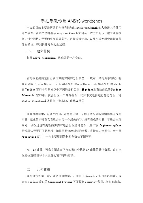
手把手教你用ANSYS workbench 本文的目的主要是帮助那些没有接触过ansys workbench的人快速上手使用这个软件。
在本文里将展示ansys workbench如何从一片空白起步,建立几何模型、划分网格、设置约束和边界条件、进行求解计算,以及在后处理中运行疲劳分析模块,得到估计寿命的全过程。
一、建立算例打开ansys workbench,这时还是一片空白。
首先我们要清楚自己要计算的算例的分析类型,一般对于结构力学领域,有静态分析(Static Structural)、动态分析(Rigid Dynamics)、模态分析(Modal)。
在Toolbox窗口中用鼠标点中算例的分析类型,将它拖出到右边白色的Project Schematic窗口中,就会出现一个算例框图。
比如本文选择进行静态分析,将Static Structural条目拖出到右边,出现A框图。
在算例框图中,有多个栏目,这些是计算一个静态结构分析算例需要完成的步骤,完成的步骤在它右边会出现一个绿色的勾,没有完成的步骤,右边会出现问号,修改过没有更新的步骤右边会出现循环箭头。
第二项EngineeringData 已经默认设置好了钢材料,如果需要修改材料的参数,直接双击点开它,会出现Properties窗口,一些主要用到的材料参数如下图所示:点中SN曲线,可在右侧或者下方的窗口中找到SN曲线的具体数据。
窗口出现的位置应该与个人设置的窗口布局有关。
二、几何建模现在进行到第三步,建立几何模型。
右键点击Grometry条目可以创建,或者在Toolbox窗口的Component Systems下面找到Geometry条目,将它拖出来,也可以创建,拖出来之后,出现一个新的框图,几何模型框图。
双击框图中的Geometry,会跳出一个新窗口,几何模型设计窗口,如下图所示:点击XYPlane,再点击创建草图的按钮,表示在XY平面上创建草图,如下图所示:右键点击XYPlane,选择Look at,可将右边图形窗口的视角旋转到XYPlane 平面上:创建了草图之后点击XYPlane下面的Sketch2(具体名字可按用户需要修改),再点击激活Sketching页面:在Sketching页面可以创建几何体,从基本的轮廓线开始创建起,我们现在右边的图形窗口中随便画一条横线:画出的横线长度是鼠标随便点出来的,并不是精确地等于用户想要的长度,甚至可能与想要的长度相差好多个数量级。
- 1、下载文档前请自行甄别文档内容的完整性,平台不提供额外的编辑、内容补充、找答案等附加服务。
- 2、"仅部分预览"的文档,不可在线预览部分如存在完整性等问题,可反馈申请退款(可完整预览的文档不适用该条件!)。
- 3、如文档侵犯您的权益,请联系客服反馈,我们会尽快为您处理(人工客服工作时间:9:00-18:30)。
ANSYS 入门教程- 加载、求解及后处理技术B2011-01-09 14:20:38| 分类:ansys | 标签:|字号大中小订阅三、施加面载荷(续)3. 在线上施加面荷载命令:SFL, LINE, Lab, V ALI, V ALJ, V AL2I, V AL2JLINE - 拟施加荷载的线号,也可为ALL 或组件名。
Lab - 面荷载标识符,结构分析为PRES。
V ALI - 线始端关键点处的面荷载值,也可为表格型边界条件的表格名。
V ALJ - 线末端关键点处的面荷载值,也可为表格型边界条件的表格名。
如为空(缺省)与V ALI 相等,否则采用输入数据。
V AL2I,VAL2J - 为复数输入时的虚部,而V ALI 和V ALJ 则为实部。
该命令仅对2D 面单元的边界(线)、轴对称单元本身、壳单元边界(线)有效,对3D 实体单元的线无效。
对于2D 面单元,其输入的面荷载值为“力/面积”;而对壳单元,其输入的面荷载值为“力/长度”,这点需要特别注意。
4. 在面上施加面荷载命令:SFA, AREA, LKEY, Lab, V ALUE, V ALUE2AREA - 拟施加面荷载的面号,也可为ALL或元件名。
LKEY - 荷载施加的面号(缺省为1)。
如果面为体单元的表面,则LKEY 将被忽略;对壳单元LKEY 可取1 或2,而其它值无效,单元帮助中有详细说明。
Lab - 面荷载标识符,结构分析为PRES。
V ALUE - 面荷载值,也可为表格名称。
V ALUE2 - 对结构分析无意义。
该命令对壳单元和3D 体单元的面施加法向面荷载,对2D 面单元无效。
5. 面荷载梯度及其加载定义面荷载梯度后,可在SF、SFE、SFL 和SFA 命令中使用。
如前所述,SFE、SFL 及SFBEAM 命令可以直接施加线性分布荷载,采用SFGRAD 命令定义荷载梯度后,使用SF 和SFA 命令施加线性分布荷载比较方便,如静水压力、圆柱体分布压力等。
示例:! EX4.9 利用荷载梯度在直角坐标系下的施加方法FINISH $ /CLEAR $ /PREP7et,1,82 $ blc4,,,10,60 ! 定义单元类型,创建面esize,2 $ amesh,all ! 定义单元尺寸,划分网格/PSF,PRES,NORM,2 ! 设置荷载显示方式sfgrad,pres,,y,0,-5 ! 定义荷载梯度,SLZER=0,沿Y 正方向递减5 单位/长度nsel,s,loc,x,0 ! 选择X=0,且Y=0~40 的节点群nsel,r,loc,y,0,40sf,all,pres,600 ! 对节点群施加面荷载,基值(Y=SLZER=0 处)为600 ! 上述荷载施加结果:Y=0 处为600,Y=40 处为600+(40-0)×(-5)=400 sfgrad,pres,,y,30,-20 ! 再重新定义梯度荷载,SLZER=30,斜率为-20nsel,s,loc,x,10 ! 选择X=10 的节点群sf,all,pres,0 ! 对节点群施加面荷载,基值(Y=SLZER=30 处)为0allsel $ eplot ! 如图4-1 所示6. 表面效应单元施加面荷载如前所述,施加具有LKEY 参数的面荷载与单元类型相关,★对于2D 面单元仅可在单元边上或边界上施加平行于单元面的荷载;★对于3D 体单元,仅可施加单元面法向面荷载;★对于3D 壳单元,可施加单元面法向面荷载和在单元边上或边界上施加平行于单元面的荷载。
但有时所要施加的荷载不属于上述情况,例如面的切向荷载或其它非法向面荷载等,此时可使用表面效应单元覆盖所要施加荷载的表面,并用这些单元作为“管道”施加所需荷载。
如2 D 面单元和3 D 单元可分别使用SURF153 单元和SURF154 单元。
示例:finish $ /clear $ /prep7et,1,solid95 $ et,2,surf154 ! 定义SOLID95 单元和表面效应单元surf 154blc4,,,10,10,40 ! 创建长方体esize,5 $ vmesh,all ! 定义单元尺寸,划分网格/psf,pres,tany,2 ! 设置压力显式方式(单元坐标系Y 切向)nsel,s,loc,y,10 ! 选择Y=10 的所有节点type,2 $ esurf ! 设置单元类型2, 生成表面效应单元esel,s,type,,2 ! 选择单元类型为2 的单元(表面效应单元)sfe,all,3,pres,,100 ! 施加LKEY=3 的面荷载(切向)allsel ! 可查看单元荷载(求解过程与SURF154 无关)四、施加体载荷在结构分析中,ANSYS 的体荷载只有温度,其标识符为TEMP。
常用体载荷命令如下表:几个主要的体荷载施加命令如下:BF, NODE, Lab, V AL1BFE, ELEM, Lab, STLOC, V AL1, V AL2, V AL3, V AL4BFK, KPOI, Lab, V AL1BFL, LINE, Lab, V AL1BFA, AREA, Lab, V AL1BFV, VOLU, Lab, V AL1其使用方法与面荷载施加命令类似,例如第1 个参数均为图素编号,也可为ALL 或组件名;第2 个参数Lab = Ui、ROTi (i = x 或 y 或 z)、TEMP 或FLUE;V AL1~VAL4 为体荷载值,其中V AL2~V AL4 为单元不同位置上的体荷载值;STLOC 为V AL1 指定一个对应的起始位置。
五、施加惯性荷载惯性荷载有加速度、角速度和角加速度。
惯性荷载没有删除命令,要删除惯性荷载,衷心将荷载值设为0 即可;且惯性载荷为斜坡荷载。
ACEL、OMEGA 和DOMEGA 命令分别用于施加在总体直角坐标系中的加速度、角速度和角加速度。
需要注意的是ACEL 命令施加的是加速度不是重力场,而重力加速度的方向与重力方向相反。
因此要施加一个-Y 方向的重力场,必须施加一个+Y 方向的加速度。
使用CGOMGA 和DCGOMG 命令定义一转动物体的加速度和角加速度,但为相对于参考坐标系转动时的物理量(该物体绕参考坐标系转动)。
CGLOC 命令用于指定参考坐标系相对于整个笛卡尔坐标系的位置。
CMOMEGA 和CMDOMGA 命令在单元元件上施加参考坐标系下的角速度和角加速度。
ANSYS 定义的三种类型转动为:①整个结构绕总体直角坐标系转动(OMEGA 和DOMEGA 命令输入);②单元元件绕参考坐标系轴的转动(CMOMEGA 和CMDOMEGA 命令);③整体直角坐标系绕加速度原点的转动(CGOMGA、DCGOMG 和CGLOC命令)。
以上三种类型转动中,可两两组合同时施加到结构上。
此处仅介绍ACEL 命令及使用方法,命令如下:命令:ACEL, ACELX, ACEL Y, ACELZ其中ACELX, ACEL Y, ACELZ 分别为总体直角坐标系X 轴、Y 轴和Z 轴的结构线加速度值。
六、施加耦合场荷载在耦合场分析中,通常将包含一个分析中的结果施加在第二个分析中作为荷载,例如可将热分析中计算得到的节点温度,作为体积荷载施加到结构分析中,形成耦合场荷载。
施加耦合场荷载的命令为LDREAD命令,该命令是从一个结果文件读出数据然后作为荷载施加到模型上。
因此该命令不仅仅在施加耦合场荷载时使用,也可用于其它分析目的,例如可用于结构分析中读入反作用力作为进一步分析的荷载等。
命令:LDREAD, Lab, LSTEP, SBSTEP, TIME, KIMG, Fname, Ext七、初应力荷载及施加初应力(Initial Stress)可以指定为一种“荷载”进行施加,但仅在静态分析和全瞬态分析中可以使用,可以用于线性分析或非线性分析。
初应力荷载只能在第一个荷载步中施加。
ANSYS 中支持初应力荷载的单元类型有:PLANE2、PLANE42、PLANE82、PLANE182、PLANE183、SOLID45、SOLID92、SOLID95、SOLID185、SOLID186、SOLID187、SHELL181、SHELL208、SHELL209、LINK180、BEAM188、BEAM189。
初应力荷载是单元坐标系下的值,如果单元坐标系与总体坐标系不同应谨慎。
初应力荷载只能在求解层施加。
初应力荷载的施加采用覆盖方式,即多次施加时后面命令结果覆盖前面的命令结果。
初应力荷载施加在被选择的单元上,如果单元选择集为空或不选择某些单元,则不施加初应力荷载到这些单元上。
主要初应力载荷命令如下表:1. 施加初始常应力荷载命令:ISTRESS, Sx, Sy, Sz, Sxy, Syz, Sxz, MAT1, MAT2, MA T3, MA T4, MA T5, MA T6, MA T7, MA T8, MA T9, MAT10Sx,Sy,Sz,Sxy,Syz,Sxz - 初始的常应力值。
MAT1~MAT10 - 初应力拟施加到的材料编号,如没有指定,则施加到所有材料上。
该命令对所选择的单元施加一组初始常应力值。
2. 从文件施加初应力荷载命令:ISFILE, Option, Fname, Ext, --, LOC, MA T1, MAT2, MAT3, MAT4, MAT5, MAT6, MAT7, MA T8, MA T9, MAT10Option - 初应力荷载操作控制参数,其值可取:=READ(缺省):从文件读入初应力数据;=LIST:列出已经读入的初应力;=DELE:删除已经读入的初应力。
Fname - 当Option=READ 时,Fname 为一目录和文件名。
当Option=LIST 或DELE时,Fname 为列表或删除单元编号上的初应力。
Ext - 文件扩展名或层号,当Fname 为空时,Ext 缺省为“IST”。
如Option=LIST 或DELE 则Ext 为层壳单元的层号。
LOC - 总体位置标志,确定每个单元内初应力要施加的位置,其值可取:=0(缺省):在单元质心上施加初应力;=1:单元积分点上施加初应力;=2:在单元指定位置上施加初应力。
即由初应力文件确定将初应力荷载施加到什么位置,此时各个单元施加的位置可以不相同。
=3:常应力状态。
用初应力文件中的第一个应力数据将所有单元初始化为一个常应力。
MAT1~MAT10 - 初应力拟施加到的材料编号。
该命令对所选择的单元施加初应力荷载,初应力的单元号与所选择的单元号相对应。
3. 生成初应力文件命令:ISWRITE, Switch其中Switch 参数控制初应力文件是否生成文件,其中可取:ON:以工作文件及扩展名IST 生成初应力文件,并写入数据;OFF:不生成初应力文件。