spss_数据正态分布检验方法及意义
SPSS学习系列19. 正态性检验
19. 正态性检验实际中,经常需要检验数据是否服从正态分布。
一、Kolmogorov-Smirnov(K - S) 单样本检验这是一种分布拟合优度检验,即将一个变量的累积分布函数与特定分布进行比较。
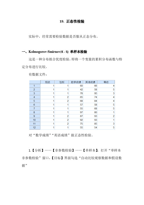
有数据文件:对“数学成绩”“英语成绩”做正态性检验。
1.【分析】——【非参数检验】——【单样本】,打开“单样本非参数检验”窗口,【目标】界面勾选“自动比较观察数据和假设数据”2.【字段】界面,勾选“使用定制字段分配”,将要检验的变量“数学成绩”“英语成绩”选入【检验字段】框,3. 【设置】界面,选择“自定义检验”,勾选“检验观察分布和假设分布(Kolmogorov-Smimov检验)”点【选项】,打开“Kolmogorov-Smimov检验选项”子窗口,选择“正态分布”,勾选“使用样本数据”,点【确定】回到原窗口,点【运行】得到结果说明:样本量大于50用Kolmogorov-Smirnov检验,样本量小于50用Shapiro-Wilk检验;原假设H0:服从正态分布;H1:不服从正态分布。
P值<0.05, 拒绝原假设H0;P值>0.05, 接受原假设H0, 即服从正态分布;本例中,“数学成绩”、“英语成绩”的P值都>0.05, 故服从正态分布。
双击上面结果可以看到更详细的检验结果:注:类似的操作也可以检验数据是否服从“二项、均匀、指数、泊松”等分布。
二、用“旧对话框”进行上述检验1.【分析】——【非参数检验】——【旧对话框】——【1-样本K-S】,打开“单样本Kolmogorov-Smirnov检验”窗口,将要检验的变量选入【检验变量列表】框,【检验分布】勾选“常规”,2.点【精确】,打开“精确检验”窗口,勾选“精确”,“仅渐进法”——只计算检验统计量的渐近分布的近似概率值,而不计算确切概率,适用用样本量较大,P值远离α=0.05,节省计算时间,否则可能结果偏差较大;“Monte Carlo”——利用模拟抽样方法求得P值的近似无偏估计,适合大样本数据,节省计算时间;“精确”——计算精确的概率值(P值)。
spss判断是否符合正态分布
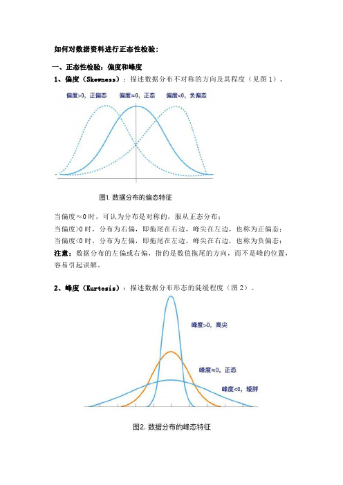
如何对数据资料进行正态性检验:一、正态性检验:偏度和峰度1、偏度(Skewness):描述数据分布不对称的方向及其程度(见图1)。
当偏度≈0时,可认为分布是对称的,服从正态分布;当偏度>0时,分布为右偏,即拖尾在右边,峰尖在左边,也称为正偏态;当偏度<0时,分布为左偏,即拖尾在左边,峰尖在右边,也称为负偏态;注意:数据分布的左偏或右偏,指的是数值拖尾的方向,而不是峰的位置,容易引起误解。
2、峰度(Kurtosis):描述数据分布形态的陡缓程度(图2)。
当峰度≈0时,可认为分布的峰态合适,服从正态分布(不胖不瘦);当峰度>0时,分布的峰态陡峭(高尖);当峰度<0时,分布的峰态平缓(矮胖);利用偏度和峰度进行正态性检验时,可以同时计算其相应的Z评分(Z-score),即:偏度Z-score=偏度值/标准误,峰度Z-score=峰度值/标准误。
在α=0.05的检验水平下,若Z-score在±1.96之间,则可认为资料服从正态分布。
了解偏度和峰度这两个统计量的含义很重要,在对数据进行正态转换时,需要将其作为参考,选择合适的转换方法。
3、SPSS操作方法以分析某人群BMI的分布特征为例。
(1) 方法一选择Analyze → Descriptive Statistics → Frequencies将BMI选入Variable(s)框中→点击Statistics →在Distribution框中勾选Skewness和Kurtosis(2) 方法二选择Analyze → Descriptive Statistics → Descriptives将BMI选入Variable(s)框中→点击Options →在Distribution框中勾选Skewness和Kurtosis4、结果解读在结果输出的Descriptives部分,对变量BMI进行了基本的统计描述,同时给出了其分布的偏度值0.194(标准误0.181),Z-score = 0.194/0.181 = 1.072,峰度值0.373(标准误0.360),Z-score = 0.373/0.360 = 1.036。
SPSS统计分析1:正态分布检验
正态分布检验一、正态检验的必要性[1]当对样本是否服从正态分布存在疑虑时,应先进行正态检验;如果有充分的理论依据或根据以往积累的信息可以确认总体服从正态分布时,不必进行正态检验。
当然,在正态分布存疑的情况下,也就不能采用基于正态分布前提的参数检验方法,而应采用非参数检验。
二、图示法1、P-P图以样本的累计频率作为横坐标,以安装正态分布计算的相应累计概率作为纵坐标,把样本值表现为直角坐标系中的散点。
如果资料服从整体分布,则样本点应围绕第一象限的对角线分布。
2、Q-Q图以样本的分位数作为横坐标,以按照正态分布计算的相应分位点作为纵坐标,把样本表现为指教坐标系的散点。
如果资料服从正态分布,则样本点应该呈一条围绕第一象限对角线的直线。
以上两种方法以Q-Q图为佳,效率较高。
3、直方图判断方法:是否以钟形分布,同时可以选择输出正态性曲线。
4、箱式图判断方法:观测离群值和中位数。
5、茎叶图类似与直方图,但实质不同。
三、计算法1、峰度(Kurtosis)和偏度(Skewness)(1)概念解释峰度是描述总体中所有取值分布形态陡缓程度的统计量。
这个统计量需要与正态分布相比较,峰度为0表示该总体数据分布与正态分布的陡缓程度相同;峰度大于0表示该总体数据分布与正态分布相比较为陡峭,为尖顶峰;峰度小于0表示该总体数据分布与正态分布相比较为平坦,为平顶峰。
峰度的绝对值数值越大表示其分布形态的陡缓程度与正态分布的差异程度越大。
峰度的具体计算公式为:注:SD就是标准差σ。
峰度原始定义不减3,在SPSS中为分析方便减3后与0作比较。
偏度与峰度类似,它也是描述数据分布形态的统计量,其描述的是某总体取值分布的对称性。
这个统计量同样需要与正态分布相比较,偏度为0表示其数据分布形态与正态分布的偏斜程度相同;偏度大于0表示其数据分布形态与正态分布相比为正偏或右偏,即有一条长尾巴拖在右边,数据右端有较多的极端值;偏度小于0表示其数据分布形态与正态分布相比为负偏或左偏,即有一条长尾拖在左边,数据左端有较多的极端值。
SPSS学习笔记-正态性检验

如何在spss中进行正态分布检验一、图示法1、P-P图以样本的累计频率作为横坐标,以安装正态分布计算的相应累计概率作为纵坐标,把样本值表现为直角坐标系中的散点。
如果资料服从整体分布,则样本点应围绕第一象限的对角线分布。
2、Q-Q图以样本的分位数作为横坐标,以按照正态分布计算的相应分位点作为纵坐标,把样本表现为指教坐标系的散点。
如果资料服从正态分布,则样本点应该呈一条围绕第一象限对角线的直线。
以上两种方法以Q-Q图为佳,效率较高。
3、直方图判断方法:是否以钟形分布,同时可以选择输出正态性曲线。
4、箱式图判断方法:观测离群值和中位数。
5、茎叶图类似与直方图,但实质不同。
二、计算法1、偏度系数(Skewness)和峰度系数(Kurtosis)计算公式:g1表示偏度,g2表示峰度,通过计算g1和g2及其标准误σg1及σg2然后作U检验。
两种检验同时得出U<U0.05=1.96,即p>0.05的结论时,才可以认为该组资料服从正态分布。
由公式可见,部分文献中所说的“偏度和峰度都接近0……可以认为……近似服从正态分布”并不严谨。
2、非参数检验方法非参数检验方法包括Kolmogorov-Smirnov检验(D检验)和Shapiro- Wilk(W检验)。
SAS中规定:当样本含量n≤2000时,结果以Shapiro – Wilk(W检验)为准,当样本含量n >2000时,结果以Kolmogorov – Smirnov(D检验)为准。
SPSS中则这样规定:(1)如果指定的是非整数权重,则在加权样本大小位于3和50之间时,计算Shapiro-Wilk统计量。
对于无权重或整数权重,在加权样本大小位于3和5000之间时,计算该统计量。
由此可见,部分SPSS教材里面关于“Shapiro – Wilk适用于样本量3-50之间的数据”的说法是在是理解片面,误人子弟。
(2)单样本Kolmogorov-Smirnov检验可用于检验变量(例如income)是否为正态分布。
SPSS数据的参数检验和方差分析
SPSS数据的参数检验和方差分析参数检验和方差分析是统计学中常用的两种分析方法。
本文将详细介绍SPSS软件中如何进行参数检验和方差分析,并提供一个示例来说明具体的操作步骤。
参数检验(Parametric Tests)适用于已知总体分布类型的数据,通过比较样本数据与总体参数之间的差异,来判断样本数据是否与总体相符。
常见的参数检验包括:1. 单样本t检验(One-sample t-test):用于比较一个样本的均值是否与总体均值相等。
2. 独立样本t检验(Independent samples t-test):用于比较两个独立样本的均值是否相等。
3. 配对样本t检验(Paired samples t-test):用于比较两个相关样本的均值是否相等。
4. 卡方检验(Chi-square test):用于比较两个或多个分类变量之间的关联性。
接下来,将以一个具体的实例来说明SPSS软件中如何进行单样本t检验和卡方检验。
实例:假设我们有一个数据集,记录了一所学校不同班级学生的身高信息。
我们想要进行以下两种分析:1. 单样本t检验:假设我们想要检验学生身高平均值是否等于169cm(假设总体均值为169cm)。
步骤如下:b.选择“分析”菜单,然后选择“比较均值”下的“单样本t检验”。
c.在弹出的对话框中,选择需要进行t检验的变量(身高),并将值169输入到“测试值”框中。
d.点击“确定”按钮,SPSS将生成t检验的结果,包括样本均值、标准差、t值和p值。
2.卡方检验:假设我们想要检验学生身高与体重之间是否存在关联。
步骤如下:a.打开SPSS软件,并导入数据集。
b.选择“分析”菜单,然后选择“非参数检验”下的“卡方”。
c.在弹出的对话框中,选择需要进行卡方检验的两个变量(身高和体重)。
d.点击“确定”按钮,SPSS将生成卡方检验的结果,包括卡方值、自由度和p值。
方差分析(Analysis of Variance,简称ANOVA)用于比较两个或以上样本之间的均值差异。
spss正态分布检验方法
spss正态分布检验方法SPSS正态分布检验方法。
SPSS(Statistical Package for the Social Sciences)是一种统计分析软件,广泛应用于社会科学、生物医学、教育研究等领域。
在数据分析过程中,正态分布检验是一项重要的统计方法,用于检验数据是否符合正态分布。
本文将介绍在SPSS中进行正态分布检验的方法及步骤。
SPSS正态分布检验方法主要包括两种统计检验,Shapiro-Wilk 检验和Kolmogorov-Smirnov检验。
Shapiro-Wilk检验是一种较为常用的正态性检验方法,适用于样本量较小(通常小于50)的情况。
在SPSS中,进行Shapiro-Wilk检验的步骤如下:1. 打开SPSS软件,导入需要进行正态分布检验的数据文件。
2. 选择“分析”菜单中的“描述统计”选项,然后在弹出的对话框中选择“探索性数据分析”。
3. 在“探索性数据分析”对话框中,将需要进行正态性检验的变量移动到“因子”框中。
4. 点击“统计”按钮,在弹出的对话框中勾选“Shapiro-Wil k”复选框。
5. 点击“确定”按钮,SPSS将输出Shapiro-Wilk检验的结果,包括统计量W和显著性水平。
Kolmogorov-Smirnov检验适用于样本量较大的情况,其原理是通过比较累积分布函数来检验数据是否符合正态分布。
在SPSS中进行Kolmogorov-Smirnov检验的步骤如下:1. 打开SPSS软件,导入需要进行正态分布检验的数据文件。
2. 选择“分析”菜单中的“非参数检验”选项,然后在弹出的对话框中选择“单样本K-S检验”。
3. 在“单样本K-S检验”对话框中,将需要进行正态性检验的变量移动到“测试变量列表”框中。
4. 点击“确定”按钮,SPSS将输出Kolmogorov-Smirnov检验的结果,包括统计量D和显著性水平。
在进行正态分布检验时,需要注意以下几点:1. 正态性检验是基于样本数据进行的统计推断,结果受样本量的影响。
SPSS数据分析protocol
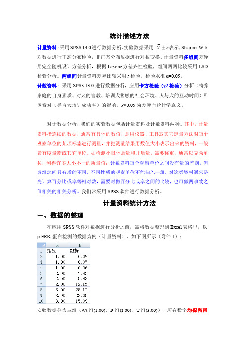
统计描述方法计量资料:采用SPSS 13.0进行数据分析,实验数据采用 X ±s表示,Shapiro-Wilk 对数据进行正态分布检验,非正态分布数据进行对数变换。
计量资料多组间差异用完全随机设计方差分析,根据Levene方差齐性检验,组间两两比较采用LSD 检验分析。
两组间计量资料差异比较采用t检验。
检验水准α=0.05。
计数资料:采用SPSS 13.0进行数据分析,应用卡方检验(χ2检验)分析(寄养家庭的自身素质、对犬的管教、培训犬接触的社会环境、人与犬的互动时间)四因素对(导盲犬培训成功率)的影响。
P<0.05为差异有统计学意义。
对于数据分析,我们的实验数据包括计量资料及计数资料两种。
其中,计量资料指连续的数据,通常有具体的数值,是用仪器、工具或其它定量方法对每个观察单位的某项标志进行测量,并把测量结果用数值大小表示出来的资料,一般带有度量衡或其它单位。
如检测小鼠体质量和肝质量,需要称重,通常以克为单位,测得许多大小不一的质量值;计数资料每个观察单位之间没有量的差别,但各组之间具有质的不同,不同性质的观察单位不能归入一组。
对这类资料通常是先计算百分比或率等相对数,需要时做百分比或率之间的比较,也可做两事物之间相关的相关分析。
我们常采用SPSS软件进行数据分析。
计量资料统计方法一、数据的整理在应用SPSS软件对数据进行分析之前,需将数据整理到Excel表格里,以p-ERK蛋白检测的数据为例(计量资料),如下图所示(附件1):实验数据分为三组(Wt组(1.00),P组(2.00),T组(3.00)),所有数字均保留两位有效数字。
标明组别和数据字样,以利于后期统计分析。
二、正态分布检验保存并关闭Excel,打开SPSS软件,打开保存的数据。
在对数据进行统计之前先进行正态分布检验,正态分布检验包括小样本Shapiro-Wilk检验(2000以下)或大样本Kolmogorov-Smirnv检验(2000以上)。
正态分布检验的3大步骤及结果处理spss
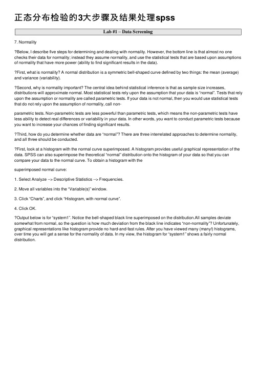
正态分布检验的3⼤步骤及结果处理spss7. NormalityBelow, I describe five steps for determining and dealing with normality. However, the bottom line is that almost no one checks their data for normality; instead they assume normality, and use the statistical tests that are based upon assumptions of normality that have more power (ability to find significant results in the data).First, what is normality A normal distribution is a symmetric bell-shaped curve defined by two things: the mean (average) and variance (variability).Second, why is normality important The central idea behind statistical inference is that as sample size increases, distributions will approximate normal. Most statistical tests rely upon the assumption that your data is “normal”. Tests that rely upon the assumption or normality are called parametric tests. If your data is not normal, then you would use statistical tests that do not rely upon the assumption of normality, call non-parametric tests. Non-parametric tests are less powerful than parametric tests, which means the non-parametric tests have less ability to detect real differences or variability in your data. In other words, you want to conduct parametric tests because you want to increase your chances of finding significant results.Third, how do you determine whether data are “normal” There are three interrelated approaches to determine normality, and all three should be conducted.First, look at a histogram with the normal curve superimposed. A histogram provides useful graphical representation of the data. SPSS can also superimpose the theoretical “normal” distribution onto the histogram of your data so that you can compare your data to the normal curve. To obtain a histogram with thesuperimposed normal curve:1. Select Analyze --> Descriptive Statistics --> Frequencies.2. Move all variables into the “Variable(s)” window.3. Click “Charts”, and click “Histogram, with normal curve”.4. Click OK.Output below is for “system1”. Notice the bell-shaped black line superimposed on the distribution.All samples deviate somewhat from normal, so the question is how much deviation from the black line indicates “non-normality”? Unfortunately, graphical representations like histogram provide no hard-and-fast rules. After you have viewed many (many!) histograms, over time you will get a sense for the normality of data. In my view, the histogram for “system1” shows a fairly normal distribution.Second, look at the values of Skewness and Kurtosis. Skewness involves the symmetry of the distribution.Skewness that is normal involves a perfectly symmetric distribution. A positively skewed distribution has scores clustered to the left, with the tail extending to the right. A negatively skewed distribution has scores clustered to the right, with the tail extending to the left. Kurtosis involves the peakedness of the distribution.Kurtosis that is normal involves a distribution that is bell-shaped and not too peaked or flat. Positive kurtosis is indicated by a peak. Negative kurtosis is indicated by a flat distribution. Descriptive statistics about skewness and kurtosis can be found by using either the Frequencies, Descriptives, or Explore commands. I like to use the “Explore” command because it provides other useful information about normality, so1. Select Analyze --> Descriptive Statistics --> Explore.2. Move all variables into the “Variable(s)” window.3. Click “Plots”, and un click “Stem-and-leaf”4. Click OK.Descriptives box tells you descriptive statistics about the variable, including the value of Skewness and Kurtosis, with accompanying standard error for each. Both Skewness and Kurtosis are 0 in a normaldistribution, so the farther away from 0, the more non-normal the distribution. The question is “how much”skew or kurtosis render the data non-normal? This is an arbitrary determination, and sometimes difficult to interpret using the values of Skewness and Kurtosis. Luckily, there are more objective tests of normality, described next.Third, the descriptive statistics for Skewness and Kurtosis are not as informative as established tests for normality that take into account both Skewness and Kurtosis simultaneously. The Kolmogorov-Smirnov test (K-S) and Shapiro-Wilk (S-W) test are designed to test normality by comparing your data to a normaldistribution with the same mean and standard deviation of your sample:1. Select Analyze --> Descriptive Statistics --> Explore.2. Move all variables into the “Variable(s)” window.3. Click “Plots”, and un click “Stem-and-leaf”, and click “Normality plots with tests”.4. Click OK.“Test of Normality” box gives the K-S and S-W test results. If the test is NOT significant, then the data are normal, so any value above .05 indicates normality. If the test is significant (less than .05), then the data are non-normal. In this case, both tests indicate the data are non-normal. However, one limitation of the normality tests is that the larger the sample size, the more likely to get significant results. Thus, you may get significant results with only slight deviations from normality. In this case, our sample size is large (n=327) so thesignificance of the K-S and S-W tests may only indicate slight deviations from normality. You need to eyeball your data (using histograms) to determine for yourself if the data rise to the level of non-normal.“Normal Q-Q Plot” provides a graphical way to determine the level of normality. The black line indicates the values your sample should adhere to if the distribution was normal. The dots are your actual data. If the dots fall exactly on the black line, then your data are normal. If they deviate from the black line, your data are non-normal. In this case, you can see substantial deviation from the straight black line.Fourth, if your data are non-normal, what are your options to deal with non-normality You have four basic options.a.Option 1 is to leave your data non-normal, and conduct the parametric tests that rely upon theassumptions of normality. Just because your data are non-normal, does not instantly invalidate theparametric tests. Normality (versus non-normality) is a matter of degrees, not a strict cut-off point.Slight deviations from normality may render the parametric tests only slightly inaccurate. The issue isthe degree to which the data are non-normal.b.Option 2 is to leave your data non-normal, and conduct the non-parametric tests designed for non-normal data.c.Option 3 is to conduct “robust” tests. There is a growing branch of statistics called “robust” tests thatare just as powerful as parametric tests but account for non-normality of the data.d.Option 4 is to transform the data. Transforming your data involving using mathematical formulas tomodify the data into normality.Fifth, how do you transform your data into “normal” data There are different types of transformations based upon the type of non-normality. For example, see handout “Figure 8.1” on the last page of this document that shows six types of non-normality (e.g., 3 positive skew that are moderate, substantial, and severe; 3 negative skew that are moderate, substantial, and severe). Figure 8.1 also shows the type of transformation for each type of non-normality. Transforming the data involves using the “Compute” function to create a new variable (the new variable is the old variable transformed by the mathematical formula):1. Select Transform --> Compute Variable2. Type the name of the new variable you wan t to create, such as “transform_system1”.3. Select the type of transformation from the “Functions” list, and double-click.4. Move the (non-normal) variable name into the place of the question mark “?”.5. Click OK.The new variable is reproduced in the last column in the “Data view”.Now, check that the variable is normal by using the tests described above.If the variable is normal, then you can start conducting statistical analyses of that variable.If the variable is non-normal, then try other transformations.。
- 1、下载文档前请自行甄别文档内容的完整性,平台不提供额外的编辑、内容补充、找答案等附加服务。
- 2、"仅部分预览"的文档,不可在线预览部分如存在完整性等问题,可反馈申请退款(可完整预览的文档不适用该条件!)。
- 3、如文档侵犯您的权益,请联系客服反馈,我们会尽快为您处理(人工客服工作时间:9:00-18:30)。
spss 数据正态分布检验方法及意义判读要观察某一属性的一组数据是否符合正态分布,可以有两种方法(目前我知道这两种,并且这两种方法只是直观观察,不是定量的正态分布检验):1:在spss里的基本统计分析功能里的频数统计功能里有对某个变量各个观测值的频数直方图中可以选择绘制正态曲线。
具体如下:Analyze-----Descriptive S tatistics-----Frequencies,打开频数统计对话框,在Statistics里可以选择获得各种描述性的统计量,如:均值、方差、分位数、峰度、标准差等各种描述性统计量。
在Charts里可以选择显示的图形类型,其中Histograms选项为柱状图也就是我们说的直方图,同时可以选择是否绘制该组数据的正态曲线(With nor ma curve),这样我们可以直观观察该组数据是否大致符合正态分布。
如下图:从上图中可以看出,该组数据基本符合正态分布。
2:正态分布的Q-Q图:在spss里的基本统计分析功能里的探索性分析里面可以通过观察数据的q-q图来判断数据是否服从正态分布。
具体步骤如下:Analyze-----Descriptive Statistics-----Explore打开对话框,选择Plots选项,选择Normality plots with tests选项,可以绘制该组数据的q-q 图。
图的横坐标为改变量的观测值,纵坐标为分位数。
若该组数据服从正态分布,则图中的点应该靠近图中直线。
纵坐标为分位数,是根据分布函数公式F(x)=i/n+1得出的.i为把一组数从小到大排序后第i个数据的位置,n为样本容量。
若该数组服从正态分布则其q-q图应该与理论的q-q图(也就是图中的直线)基本符合。
对于理论的标准正态分布,其q-q图为y=x直线。
非标准正态分布的斜率为样本标准差,截距为样本均值。
如下图:如何在spss中进行正态分布检验1(转)(2009-07-22 11:11:57)标签:杂谈一、图示法1、P-P图以样本的累计频率作为横坐标,以安装正态分布计算的相应累计概率作为纵坐标,把样本值表现为直角坐标系中的散点。
如果资料服从整体分布,则样本点应围绕第一象限的对角线分布。
2、Q-Q图以样本的分位数作为横坐标,以按照正态分布计算的相应分位点作为纵坐标,把样本表现为指教坐标系的散点。
如果资料服从正态分布,则样本点应该呈一条围绕第一象限对角线的直线。
以上两种方法以Q-Q图为佳,效率较高。
3、直方图判断方法:是否以钟形分布,同时可以选择输出正态性曲线。
4、箱式图判断方法:观测离群值和中位数。
5、茎叶图类似与直方图,但实质不同。
二、计算法1、偏度系数(Skewness)和峰度系数(Kurtosis)计算公式:g1表示偏度,g2表示峰度,通过计算g1和g2及其标准误σg1及σg2然后作U检验。
两种检验同时得出U<U0.05=1.96,即p>0.05的结论时,才可以认为该组资料服从正态分布。
由公式可见,部分文献中所说的“偏度和峰度都接近0……可以认为……近似服从正态分布”并不严谨。
2、非参数检验方法非参数检验方法包括Kolmogorov-Smirnov检验(D检验)和Shapiro- Wilk(W检验)。
SAS中规定:当样本含量n≤2000时,结果以Shapiro –Wilk(W检验)为准,当样本含量n >2000时,结果以Kolmogorov –Smirnov(D检验)为准。
SPSS中则这样规定:(1)如果指定的是非整数权重,则在加权样本大小位于3和50之间时,计算Shapiro-Wilk统计量。
对于无权重或整数权重,在加权样本大小位于3和5000之间时,计算该统计量。
由此可见,部分SPSS教材里面关于“Shapiro –Wilk适用于样本量3-50之间的数据”的说法是在是理解片面,误人子弟。
(2)单样本Kolmogorov-Smirnov 检验可用于检验变量(例如income)是否为正态分布。
对于此两种检验,如果P值大于0.05,表明资料服从正态分布。
三、SPSS操作示例SPSS中有很多操作可以进行正态检验,在此只介绍最主要和最全面最方便的操作:1、工具栏--分析—描述性统计—探索性2、选择要分析的变量,选入因变量框内,然后点选图表,设置输出茎叶图和直方图,选择输出正态性检验图表,注意显示(Display)要选择双项(Both)。
3、Output结果(1)Descriptives:描述中有峰度系数和偏度系数,根据上述判断标准,数据不符合正态分布。
S k=0,K u=0时,分布呈正态,Sk>0时,分布呈正偏态,Sk<0时,分布呈负偏态,时,Ku>0曲线比较陡峭,Ku<0时曲线比较平坦。
由此可判断本数据分布为正偏态(朝左偏),较陡峭。
(2)Tests of Normality:D检验和W检验均显示数据不服从正态分布,当然在此,数据样本量为1000,应以W检验为准。
(3)直方图直方图验证了上述检验结果。
(4)此外还有茎叶图、P-P图、Q-Q图、箱式图等输出结果,不再赘述。
结果同样验证数据不符合正态分布。
spss 判断两组数据的相关性(已使用)(2009-07-22 13:07:34)标签:杂谈两组体重数据:先要为数据分组2.0 3000.02.0 3700.02.0 2900.02.0 3200.02.0 2950.02.0 3100.02.0 700.02.0 3200.02.0 2500.02.0 3650.02.0 4600.0 2.0 2700.0 2.0 2500.0 2.0 3150.0 2.0 3500.0 2.0 3800.0 2.0 2800.0 2.0 2400.0 2.0 3600.0 2.0 3200.0 2.0 1770.0 2.0 1450.0 2.0 1700.0 2.0 3250.0 2.0 2700.0 2.0 3000.0 2.0 2250.0 2.0 2150.0 2.0 2450.0 2.0 1600.0 2.0 3100.0 2.0 4050.0 2.0 4250.0 2.0 2900.0 2.0 3250.0 2.0 3750.0 2.0 3500.0 2.0 4100.0 2.0 3100.0 2.0 2400.0 2.0 3250.0 2.0 2600.0 2.0 3100.0 2.0 3400.0 1.0 2400.0 1.0 2100.0 1.0 3000.01.0 4000.01.0 2200.01.0 1400.01.0 3000.01.0 3200.01.0 3600.01.0 2850.01.0 2850.01.0 3300.01.0 3500.01.0 3900.01.0 3250.01.0 3800.01.0 2800.01.0 3500.01.0 2650.01.0 2350.01.0 1400.01.0 2900.01.0 2550.01.0 2850.01.0 3300.01.0 2250.01.0 2500.0使用命令: spss的t检验:菜单Analyze->Compare Means->Independent-Samples T Test运行结果:经方差齐性检验: F= 0.393 P=0.532,即两方差齐。
(因为p大于0.05)所以选用 t检验的第一行方差齐情况下的t检验的结果:就是选用方差假设奇的结果所以,t=0.644 , p=0.522, 没有显著性差异。
(因为p < 0.05表示差异有显著性)。
均值相差:113.30159解释:使用compare means里的independent smaples T test,检验结果里的 Levene\'s Test for Equality of Variances就是对方差齐性的检验,如果P值大于0.05则认为是方差齐,统计量为F= S1^2/S^2 ~ F(n1-1,n2-1) ,显著水平一般为0.05,0.01,原假设H0:方差相等。
方差分析(Anaylsis of Variance, ANOVA)要求各组方差整齐,不过一般认为,如果各组人数相若,就算未能通过方差整齐检验,问题也不大。
One-Way ANOVA对话方块中,点击Options…(选项…)按扭,勾Homogeneity-of-variance即可。
它会产生Levene、Cochran C、Bartlett-Box F等检验值及其显著性水平P值,若P值<于0.05,便拒绝方差整齐的假设。
顺带一提,Cochran和Bartlett检定对非正态性相当敏感,若出现「拒绝方差整齐」的检测结果,或因这原因而做成。
Statistics菜单->Compare Means->Independent-samples T Test..再看看结果中p值的大小是否<.05,若然即达显著水平。
SPSS学习笔记描述样本数据一般的,一组数据拿出来,需要先有一个整体认识。
除了我们平时最常用的集中趋势外,还需要一些离散趋势的数据。
这方面EXCEL就能一次性的给全了数据,但对于SPSS,就需要用多个工具了,感觉上表格方面不如EXCEL好用。
个人感觉,通过描述需要了解整体数据的集中趋势和离散趋势,再借用各种图观察数据的分布形态。
对于SPSS提供的OLAP cubes(在线分析处理表),Case Summary(观察值摘要分析表),Descriptives (描述统计)不太常用,反喜欢用Frequencies(频率分析),Basic Table(基本报表),Crosstabs(列联表)这三个,另外再配合其它图来观察。
这个可以根据个人喜好来选择。
一.使用频率分析(Frequencies)观察数值的分布。
频率分布图与分析数据结合起来,可以更清楚的看到数据分布的整体情况。
以自带文件Trends chapter 13.sav为例,选择Analyze->Descriptive Statistics->Frequencies,把hstarts选入Variables,取消在Display Frequency table前的勾,在Chart里面histogram,在Statistics选项中如图1图1分别选好均数(Mean),中位数(Median),众数(Mode),总数(Sum),标准差(Std. deviation),方差(Variance),范围(range),最小值(Minimum),最大值(Maximum),偏度系数(Skewness),峰度系数(Kutosis),按Continue返回,再按OK,出现结果如图2图2表中,中位数与平均数接近,与众数相差不大,分布良好。