数字图像处理英文版
数字图像处理-冈萨雷斯-课件(英文)Chapter11-表示与描述可编辑全文

Benefits: - Easier to understand - Require fewer memory, faster to be processed - More “ready to be used”
3 from
Lupper
Turn Right OK!
Turn Right OK!
Algorithm (cont.)
For the lower side of a convex hull
7. 8.
Put For
the i=
np-o2indtoswpnn
The First Difference of a Chain Codes
Problem of a chain code: a chain code sequence depends on a starting point.
Solution: treat a chain code as a circular sequence and redefine the starting point so that the resulting sequence of numbers forms an integer of minimum magnitude.
Remove the first and the last points from AReptpuernndLLlower to Lupper resulting in the list
LLlower
3 points from Llower
Turn Left NOK!
数字图像处理--灰度形态学 (英文)
Mathematical Morphology
L.J. van Vliet TNW-IST Quantitative Imaging
2
The basic operations are for gray-value images are, f(x) a) Complement = gray-scale inversion b) Translation: c) Offset = gray addition: d) Multiplication = gray scaling: f(x+v) f(x) + t a f(x) f1(x) À f2(x)
L.J. van Vliet TNW-IST Quantitative Imaging
18
f
f ⊗ g(σ)
dytB f
tetB f
Segmentation: Thresholding
L.J. van Vliet TNW-IST Quantitative Imaging
19
Divide the image into objects and background
4
Local MIN filter
[ εB f ]( x ) = min f ( x + β )
β ∈B
a
f(x)
minf(a,5)
g(x)
x
minf(a,9)
Opening & Top Hat
L.J. van Vliet TNW-IST Quantitative Imaging
5
Opening (or lower-envelope): min-filter followed by max-filter.
数字图像处理,冈萨雷斯,课件英文版Chapter06 彩色图像处理
(Images from Rafael C. Gonzalez and Richard E. Wood, Digital Image Processing, 2nd Edition.
RGB Safe-color Cube
The RGB Cube is divided into 6 intervals on each axis to achieve the total 63 = 216 common colors. However, for 8 bit color representation, there are the total 256 colors. Therefore, the remaining 40 colors are left to OS.
C 1 R M 1 G Y 1 B
HSI Color Model
RGB, CMY models are not good for human interpreting HSI Color model: Hue: Dominant color Saturation: Relative purity (inversely proportional to amount of white light added) Intensity: Brightness Color carrying information
(Images from Rafael C. Gonzalez and Richard E. Wood, Digital Image Processing, 2nd Edition.
RGB Color Cube
R = 8 bits G = 8 bits B = 8 bits Color depth 24 bits = 16777216 colors
数字图像处理论文中英文对照资料外文翻译文献
第 1 页中英文对照资料外文翻译文献原 文To image edge examination algorithm researchAbstract :Digital image processing took a relative quite young discipline,is following the computer technology rapid development, day by day obtains th widespread application.The edge took the image one kind of basic characteristic,in the pattern recognition, the image division, the image intensification as well as the image compression and so on in the domain has a more widesp application.Image edge detection method many and varied, in which based on brightness algorithm, is studies the time to be most long, the theory develo the maturest method, it mainly is through some difference operator, calculates its gradient based on image brightness the change, thus examines the edge, mainlyhas Robert, Laplacian, Sobel, Canny, operators and so on LOG 。
chapter_1

•Lecturer:–盛蕴–Tel: 54345185–Email: ysheng@–Addr.: 华东师范大学闵行校区信息楼612室•Aims–To understand Digital Image Processing (DIP) and its relevant algorithms, which serve as basis of many other applications.–To be able to implement these DIP algorithms with MATLAB. •Assignments: N•Assessment–Assignment + Final Design(?)–60% + 40% or 100%1.《数字图像处理数字图像处理((第3版)()(英文版英文版英文版)》,)》,)》,Rafael C. Gonzalez & Richard E. Woods Rafael C. Gonzalez & Richard E. Woods著,电子工业出版社电子工业出版社201020102010年影印年影印年影印。
2.《数字图像处理数字图像处理((MATLAB MATLAB版版)()(英文版英文版英文版)》,)》,)》,Rafael C. Gonzalez & Richard E. Woods Rafael C. Gonzalez & Richard E. Woods著,电子工业出版社电子工业出版社200920092009年影印年影印年影印。
English = Kit ?•Digital image fundamentals (4 hrs)•Image enhancement in spatial domain (6 hrs)•Image enhancement in frequency domain (6hrs)•Image restoration (4hrs)•Colour image processing (4hrs)•Wavelet and multiresolution processing (6 hrs)•Image compression (6 hrs)•Digital Image Fundamentals–History and applications of digital image processing –Fundamental steps in digital image processing–Elements of visual perception–Light and the electromagnetic spectrum–Image sensing and acquisition–Image sampling and quantization–Some basic relationships between pixels•One picture is worth more than ten thousand words•无图无真相xyf (x, y )•Picture element/image element/Pixel /Pels •Intensity /Gray Level•The field of Digital Image Processing(DIP) refers to processing digital images by means of a digital computer.•Distinction among–DIP–Image Analysis–Computer Vision•Three types of computerised processes–Low-level process–Mid-level process–High-level process•DIP defined by our textbook•First application of DIPwas the picture sent by the Bartlane cable picture transmission system through submarine cable between London & NY in the early 1920s.out meaningful DIP wasduring the spaceprogramme in the early1960s.•By a US spacecraft Ranger7 in 1964.•Gamma-rays (Positron Emission Tomography)•X-rays (Computerised Tomography)•Ultraviolet band•Visible and infrared bands•Microwaves (Radar)•Radio waves (MRI)•Others (Ultrasound)λ= c/v E = hvwhere λand v are wavelength and frequency, respectively. c is the speed of light, hindicates Planck’s constant.•Most of the images in which we are interested are generated by the combination of an “illumination”source and the reflection or absorption of energy from that source by the elements of the “scene”being imaged.Image Sampling & Quantisation•Digitising the coordinate values is called sampling. •Digitising the amplitude value is called quantisation.Image Sampling & QuantisationNM•The number of intensity level L = 2k •The number of bits required to store a digitised image b=M×N×kImage Sampling & Quantisation• Spatial resolution– Line pairs per unit distance – Dots (pixels) per unit distance e.g. 4800 dpi – Measures of spatial resolution must be stated with respect to spatial units.• Intensity resolution L = 2kImage Sampling & QuantisationImage Sampling & QuantisationImage Sampling & QuantisationImage Interpolation• Interpolation– A process of using known data to estimate values at unknown locations. – Used in scaling, zooming, shrinking, transforming and geometric correction etc. – Nearest neighbour interpolation, bilinear interpolation, bicubic interpolation etc.Image InterpolationBicubic InterpolationBilinear InterpolationImage InterpolationNeighbours of a pixel• 4-neighbours of p: N4(p)p• Diagonal neighbours: ND(p)p•8-neighbors = 4-neighbours+diagonal neighbours : N8(p)。
数字图像处理相关英文教材3

3HistogramsHistograms are used to depict image statistics in an easily interpreted visual format.With a histogram,it is easy to determine certain types of problems in an image,for example,it is simple to conclude if an image is properly exposed by visual inspection of its histogram.In fact,histograms are so useful that modern digital cameras often provide a real-time histogram overlay on the viewfinder(Fig.3.1)to help prevent taking poorly exposed pictures.It is important to catch errors like this at the image capture stage because poor exposure results in a permanent loss of information which it is not possible to recover later using image-processing techniques.In addition to their usefulness during image capture,histograms are also used later to improve the visual appearance of an image and as a“forensic”tool for determining what type of processing has previously been applied to an image.3.1What Is a Histogram?Histograms in general are frequency distributions,and histograms of images describe the frequency of the intensity values that occur in an image.This concept can be easily explained by considering an old-fashioned grayscale image like the one shown in Fig.3.2.A histogram h for a grayscale image I with intensity values in the range I(u,v)∈[0,K−1]would contain exactly K entries, where for a typical8bit grayscale image,K=28=256.Each individual histogram entry is defined ash(i)=the number of pixels in I with the intensity value i,W. Burger, M.J. Burge, Principles of Digital Image Processing, Undergraduate Topicsin Computer Science, DOI 10.1007/978-1-84800-191-6_3, Springer-Verlag London Limited, 2009©38 3.HistogramsFigure 3.1Digital camera back display showing a histogram overlay.Figure 3.2An 8-bit grayscale image and a histogram depicting the frequency distribution of its 256intensity values.for all 0≤i <K .More formally stated,h (i )=card (u,v )|I (u,v )=i .1(3.1)Therefore h (0)is the number of pixels with the value 0,h (1)the number of pixels with the value 1,and so forth.Finally h (255)is the number of all white pixels with the maximum intensity value 255=K −1.The result of the histogram computation is a one-dimensional vector h of length K .Figure 3.3gives an example for an image with K =16possible intensity values.Since a histogram encodes no information about where each of its individ-ual entries originated in the image,histograms contain no information about the spatial arrangement of pixels in the image.This is intentional since the 1card {...}denotes the number of elements (“cardinality”)in a set (see also p.233).3.2Interpreting Histograms 390123456789101112131415i i h (i h (i )Figure3.3Histogram vector for an image with K =16possible intensity values.The indices of the vector element i =0...15represent intensity values.The value of 10at index 2means that the image contains 10pixels of intensity value 2.Figure 3.4Three very different images with identical histograms.main function of a histogram is to provide statistical information,(e.g.,the distribution of intensity values)in a compact form.Is it possible to reconstruct an image using only its histogram?That is,can a histogram be somehow “in-verted”?Given the loss of spatial information,in all but the most trivial cases,the answer is no.As an example,consider the wide variety of images you could construct using the same number of pixels of a specific value.These images would appear different but have exactly the same histogram (Fig.3.4).3.2Interpreting HistogramsA histogram depicts problems that originate during image acquisition,such as those involving contrast and dynamic range,as well as artifacts resulting from image-processing steps that were applied to the image.Histograms are often used to determine if an image is making effective use of its intensity range (Fig.3.5)by examining the size and uniformity of the histogram’s distribution.40 3.HistogramsFigure3.5The effective intensity range.The graph depicts how often a pixel value occurs linearly(black bars)and logarithmically(gray bars).The logarithmic form makes even relatively low occurrences,which can be very important in the image,readily apparent. 3.2.1Image AcquisitionExposureHistograms make classic exposure problems readily apparent.As an example,a histogram where a large span of the intensity range at one end is largely unused while the other end is crowded with high-value peaks(Fig.3.6)is representative of an improperly exposed image.(a)(b)(c)Figure3.6Exposure errors are readily apparent in histograms.Underexposed(a),properly exposed(b),and overexposed(c)photographs.3.2Interpreting Histograms41(a)(b)(c)Figure 3.7How changes in contrast affect a histogram:low contrast(a),normal con-trast(b),high contrast(c).ContrastContrast is understood as the range of intensity values effectively used within a given image,that is the difference between the image’s maximum and minimum pixel values.A full-contrast image makes effective use of the entire range of available intensity values from a=a min...a max=0...K−1(black to white).Using this definition,image contrast can be easily read directly from the histogram.Figure3.7illustrates how varying the contrast of an image affects its histogram.Dynamic rangeThe dynamic range of an image is,in principle,understood as the number of distinct pixel values in an image.In the ideal case,the dynamic range encom-passes all K usable pixel values,in which case the value range is completely utilized.When an image has an available range of contrast a=a low...a high, witha min<a low and a high<a max,then the maximum possible dynamic range is achieved when all the intensity values lying in this range are utilized(i.e.,appear in the image;Fig.3.8).While the contrast of an image can be increased by transforming its existing values so that they utilize more of the underlying value range available,the dy-42 3.Histograms(a)(b)(c)Figure3.8How changes in dynamic range affect a histogram:high dynamic range(a), low dynamic range with64intensity values(b),extremely low dynamic range with only6 intensity values(c).namic range of an image can only be increased by introducing artificial(that is, not originating with the image sensor)values using methods such as interpola-tion(see Vol.2[6,Sec.10.3]).An image with a high dynamic range is desirable because it will suffer less image-quality degradation during image processing and compression.Since it is not possible to increase dynamic range after im-age acquisition in a practical way,professional cameras and scanners work at depths of more than8bits,often12–14bits per channel,in order to provide high dynamic range at the acquisition stage.While most output devices,such as monitors and printers,are unable to actually reproduce more than256dif-ferent shades,a high dynamic range is always beneficial for subsequent image processing or archiving.3.2.2Image DefectsHistograms can be used to detect a wide range of image defects that originate either during image acquisition or as the result of later image processing.Since histograms always depend on the visual characteristics of the scene captured in the image,no single“ideal”histogram exists.While a given histogram may be optimal for a specific scene,it may be entirely unacceptable for another. As an example,the ideal histogram for an astronomical image would likely be very different from that of a good landscape or portrait photo.Nevertheless,3.2Interpreting Histograms43 there are some general rules;for example,when taking a landscape image with a digital camera,you can expect the histogram to have evenly distributed intensity values and no isolated spikes.SaturationIdeally the contrast range of a sensor,such as that used in a camera,should be greater than the range of the intensity of the light that it receives from a scene. In such a case,the resulting histogram will be smooth at both ends because the light received from the very bright and the very dark parts of the scene will be less than the light received from the other parts of the scene.Unfortunately, this ideal is often not the case in reality,and illumination outside of the sensor’s contrast range,arising for example from glossy highlights and especially dark parts of the scene,cannot be captured and is lost.The result is a histogram that is saturated at one or both ends of its range.The illumination values lying outside of the sensor’s range are mapped to its minimum or maximum values and appear on the histogram as significant spikes at the tail ends.This typically occurs in an under-or overexposed image and is generally not avoidable when the inherent contrast range of the scene exceeds the range of the system’s sensor (Fig.3.9(a)).(a)(b)(c)Figure3.9Effect of image capture errors on histograms:saturation of high intensities(a), histogram gaps caused by a slight increase in contrast(b),and histogram spikes resulting from a reduction in contrast(c).Spikes and gapsAs discussed above,the intensity value distribution for an unprocessed image is generally smooth;that is,it is unlikely that isolated spikes(except for possible44 3.Histograms saturation effects at the tails)or gaps will appear in its histogram.It is also unlikely that the count of any given intensity value will differ greatly from that of its neighbors(i.e.,it is locally smooth).While artifacts like these are ob-served very rarely in original images,they will often be present after an image has been manipulated,for instance,by changing its contrast.Increasing the contrast(see Ch.4)causes the histogram lines to separate from each other and, due to the discrete values,gaps are created in the histogram(Fig.3.9(b)).De-creasing the contrast leads,again because of the discrete values,to the merging of values that were previously distinct.This results in increases in the corre-sponding histogram entries and ultimately leads to highly visible spikes in the histogram(Fig.3.9(c)).2Impacts of image compressionImage compression also changes an image in ways that are immediately evident in its histogram.As an example,during GIF compression,an image’s dynamic range is reduced to only a few intensities or colors,resulting in an obvious line structure in the histogram that cannot be removed by subsequent processing (Fig.3.10).Generally,a histogram can quickly reveal whether an image has ever been subjected to color quantization,such as occurs during conversion to a GIF image,even if the image has subsequently been converted to a full-color format such as TIFF or JPEG.Figure3.11illustrates what occurs when a simple line graphic with only two gray values(128,255)is subjected to a compression method such as JPEG, that is not designed for line graphics but instead for natural photographs.The histogram of the resulting image clearly shows that it now contains a large number of gray values that were not present in the original image,resulting ina poor-quality image3that appears dirty,fuzzy,and blurred.3.3Computing HistogramsComputing the histogram of an8-bit grayscale image containing intensity val-ues between0and255is a simple task.All we need is a set of256counters, one for each possible intensity value.First,all counters are initialized to zero. 2Unfortunately,these types of errors are also caused by the internal contrast“opti-mization”routines of some image-capture devices,especially consumer-type scan-ners.3Using JPEG compression on images like this,for which it was not designed,is one of the most egregious of imaging errors.JPEG is designed for photographs of natural scenes with smooth color transitions,and using it to compress iconic images with large areas of the same color results in strong visual artifacts(see,for example,Fig.1.9on p.19).3.3Computing Histograms45(a)(b)(c)Figure3.10Color quantization effects resulting from GIF conversion.The original image converted to a256color GIF image(left).Original histogram(a)and the histogram after GIF conversion(b).When the RGB image is scaled by50%,some of the lost colors are recreated by interpolation,but the results of the GIF conversion remain clearly visible in the histogram(c).(a)(b)(c)(d)Figure 3.11Effects of JPEG compression.The original image(a)contained only two different gray values,as its histogram(b)makes readily apparent.JPEG compression,a poor choice for this type of image,results in numerous additional gray values,which are visible in both the resulting image(c)and its histogram(d).In both histograms,the linear frequency(black bars)and the logarithmic frequency(gray bars)are shown.46 3.Histograms 1public class Compute_Histogram implements PlugInFilter{23public int setup(String arg,ImagePlus img){4return DOES_8G+NO_CHANGES;5}67public void run(ImageProcessor ip){8int[]H=new int[256];//histogram array9int w=ip.getWidth();10int h=ip.getHeight();1112for(int v=0;v<h;v++){13for(int u=0;u<w;u++){14int i=ip.getPixel(u,v);15H[i]=H[i]+1;16}17}18...//histogram H[]can now be used19}2021}//end of class Compute_HistogramProgram3.1ImageJ plugin for computing the histogram of an8-bit grayscale image.The setup()method returns DOES_8G+NO_CHANGES,which indicates that this plugin requires an8-bit grayscale image and will not alter it(line4).In Java,all elements of a newly instantiated array(line8)are automatically initialized,in this case to zero.Then we iterate through the image I,determining the pixel value p at each location(u,v),and incrementing the corresponding counter by one.At the end,each counter will contain the number of pixels in the image that have the corresponding intensity value.An image with K possible intensity values requires exactly K counter vari-ables;for example,since an8-bit grayscale image can contain at most256 different intensity values,we require256counters.While individual counters make sense conceptually,an actual implementation would not use K individ-ual variables to represent the counters but instead would use an array with K entries(int[256]in Java).In this example,the actual implementation as an array is straightforward.Since the intensity values begin at zero(like arrays in Java)and are all positive,they can be used directly as the indices i∈[0,N−1] of the histogram array.Program3.1contains the complete Java source code for computing a histogram within the run()method of an ImageJ plugin.At the start of Prog.3.1,the array H of type int[]is created(line8)and its elements are automatically initialized4to0.It makes no difference,at least in terms of thefinal result,whether the array is traversed in row or column 4In Java,arrays of primitives such as int,double are initialized at creation to0in the case of integer types or0.0forfloating-point types,while arrays of objects are initialized to null.3.4Histograms of Images with More than8Bits47 order,as long as all pixels in the image are visited exactly once.In contrast to Prog.2.1,in this example we traverse the array in the standard row-first order such that the outer for loop iterates over the vertical coordinates v and the inner loop over the horizontal coordinates u.5Once the histogram has been calculated,it is available for further processing steps or for being displayed.Of course,histogram computation is already implemented in ImageJ and is available via the method getHistogram()for objects of the class Image-Processor.If we use this built-in method,the run()method of Prog.3.1can be simplified topublic void run(ImageProcessor ip){int[]H=ip.getHistogram();//built-in ImageJ method...//histogram H[]can now be used}3.4Histograms of Images with More than8Bits Normally histograms are computed in order to visualize the image’s distribution on the screen.This presents no problem when dealing with images having 28=256entries,but when an image uses a larger range of values,for instance 16-and32-bit orfloating-point images(see Table1.1),then the growing number of necessary histogram entries makes this no longer practical.3.4.1BinningSince it is not possible to represent each intensity value with its own entry in the histogram,we will instead let a given entry in the histogram represent a range of intensity values.This technique is often referred to as“binning”since you can visualize it as collecting a range of pixel values in a container such as a bin or bucket.In a binned histogram of size B,each bin h(j)contains the number of image elements having values within the interval a j≤a<a j+1, and therefore(analogous to Eqn.(3.1))h(j)=card{(u,v)|a j≤I(u,v)<a j+1},for0≤j<B.(3.2) Typically the range of possible values in B is divided into bins of equal size k B=K/B such that the starting value of the interval j isa j=j·KB=j·k B.5In this way,image elements are traversed in exactly the same way that they are laid out in computer memory,resulting in more efficient memory access and with it the possibility of increased performance,especially when dealing with larger images (see also Appendix B,p.242).48 3.Histograms3.4.2ExampleIn order to create a typical histogram containing B =256entries from a 14-bitimage,you would divide the available value range if j =0...214−1into 256equal intervals,each of length k B =214/256=64,so that a 0=0,a 1=64,a 2=128,...a 255=16,320and a 256=a B =214=16,384=K .This results in the following mapping from the pixel values to the histogram bins h (0)...h (255):h (0)←0≤I (u,v )<64h (1)←64≤I (u,v )<128h (2)←128≤I (u,v )<192............h (j )←a j ≤I (u,v )<a j +1............h (255)←16320≤I (u,v )<163843.4.3ImplementationIf,as in the above example,the value range 0...K −1is divided into equal length intervals k B =K/B ,there is naturally no need to use a mapping table to find a j since for a given pixel value a =I (u,v )the correct histogram element j is easily computed.In this case,it is enough to simply divide the pixel value I (u,v )by the interval length k B ;that is,I (u,v )k B =I (u,v )K/B =I (u,v )·B K .(3.3)As an index to the appropriate histogram bin h (j ),we require an integer valuej = I (u,v )·B K,(3.4)where · denotes the floor function.6A Java method for computing histograms by “linear binning”is given in Prog.3.2.Note that all the computations from Eqn.(3.4)are done with integer numbers without using any floating-point op-erations.Also there is no need to explicitly call the floor function because the expressiona *B /Kin line 11uses integer division and in Java the fractional result of such an oper-ation is truncated,which is equivalent to applying the floor function (assuming3.5Color Image Histograms49 1int[]binnedHistogram(ImageProcessor ip){2int K=256;//number of intensity values3int B=32;//size of histogram,must be defined4int[]H=new int[B];//histogram array5int w=ip.getWidth();6int h=ip.getHeight();78for(int v=0;v<h;v++){9for(int u=0;u<w;u++){10int a=ip.getPixel(u,v);11int i=a*B/K;//integer operations only!12H[i]=H[i]+1;13}14}15//return binned histogram16return H;17}Program3.2Histogram computation using“binning”(Java method).Example of comput-ing a histogram with B=32bins for an8-bit grayscale image with K=256intensity levels. The method binnedHistogram()returns the histogram of the image object ip passed to it as an int array of size B.positive arguments).7The binning method can also be applied,in a similar way,tofloating-point images.3.5Color Image HistogramsWhen referring to histograms of color images,typically what is meant is a histogram of the image intensity(luminance)or of the individual color channels. Both of these variants are supported by practically every image-processing application and are used to objectively appraise the image quality,especially directly after image acquisition.3.5.1Intensity HistogramsThe intensity or luminance histogram h Lum of a color image is nothing more than the histogram of the corresponding grayscale image,so naturally all as-pects of the preceding discussion also apply to this type of histogram.The grayscale image is obtained by computing the luminance of the individual chan-nels of the color image.When computing the luminance,it is not sufficient to simply average the values of each color channel;instead,a weighted sum that 6 x rounds x down to the next whole number(see Appendix A,p.233).7For a more detailed discussion,see the section on integer division in Java in Ap-pendix B(p.237).50 3.Histograms takes into account color perception theory should be computed.This process is explained in detail in Chapter8(p.202).3.5.2Individual Color Channel HistogramsEven though the luminance histogram takes into account all color channels, image errors appearing in single channels can remain undiscovered.For ex-ample,the luminance histogram may appear clean even when one of the color channels is oversaturated.In RGB images,the blue channel contributes only a small amount to the total brightness and so is especially sensitive to this problem.Component histograms supply additional information about the intensity distribution within the individual color channels.When computing component histograms,each color channel is considered a separate intensity image and each histogram is computed independently of the other channels.Figure3.12 shows the luminance histogram h Lum and the three component histograms h R, h G,and h B of a typical RGB color image.Notice that saturation problems in all three channels(red in the upper intensity region,green and blue in the lower regions)are obvious in the component histograms but not in the lumi-nance histogram.In this case it is striking,and not at all atypical,that the three component histograms appear completely different from the correspond-ing luminance histogram h Lum(Fig.3.12(b)).3.5.3Combined Color HistogramsLuminance histograms and component histograms both provide useful informa-tion about the lighting,contrast,dynamic range,and saturation effects relative to the individual color components.It is important to remember that they pro-vide no information about the distribution of the actual colors in the image because they are based on the individual color channels and not the combi-nation of the individual channels that forms the color of an individual pixel. Consider,for example,when h R,the component histogram for the red channel, contains the entryh R(200)=24.Then it is only known that the image has24pixels that have a red intensity value of200.The entry does not tell us anything about the green and blue values of those pixels,which could be any valid value(∗);that is,(r,g,b)=(200,∗,∗).Suppose further that the three component histograms included the following entries:h R(50)=100,h G(50)=100,h B(50)=100.3.5Color Image Histograms 51(a)(b)h Lum(c)R (d)G (e)B(f)h R (g)h G (h)h BFigure 3.12Histograms of an RGB color image:original image (a),luminance histogram h Lum (b),RGB color components as intensity images (c–e),and the associated component histograms h R ,h G ,h B (f–h).The fact that all three color channels have saturation problems is only apparent in the individual component histograms.The spike in the distribution resulting from this is found in the middle of the luminance histogram (b).Could we conclude from this that the image contains 100pixels with the color combination(r,g,b )=(50,50,50)or that this color occurs at all?In general,no,because there is no way of ascertaining from these data if there exists a pixel in the image in which all three components have the value 50.The only thing we could really say is that the color value (50,50,50)can occur at most 100times in this image.So,although conventional (intensity or component)histograms of color im-ages depict important properties,they do not really provide any useful infor-mation about the composition of the actual colors in an image.In fact,a collection of color images can have very similar component histograms and still contain entirely different colors.This leads to the interesting topic of the com-bined histogram,which uses statistical information about the combined color components in an attempt to determine if two images are roughly similar in their color composition.Features computed from this type of histogram often52 3.Histograms form the foundation of color-based image retrieval methods.We will return to this topic in Chapter8,where we will explore color images in greater detail.3.6Cumulative HistogramThe cumulative histogram,which is derived from the ordinary histogram,is useful when performing certain image operations involving histograms;for in-stance,histogram equalization(see Sec.4.5).The cumulative histogram H isdefined asH(i)=ij=0h(j)for0≤i<K.(3.5)A particular value H(i)is thus the sum of all the values h(j),with j≤i,in the original histogram.Alternatively,we can define H recursively(as implemented in Prog.4.2on p.66):H(i)=h(0)for i=0H(i−1)+h(i)for0<i<K.(3.6)The cumulative histogram H(i)is a monotonically increasing function with amaximum valueH(K−1)=K−1j=0h(j)=M·N;(3.7)that is,the total number of pixels in an image of width M and height N.Figure 3.13shows a concrete example of a cumulative histogram.The cumulative histogram is useful not primarily for viewing but as a sim-ple and powerful tool for capturing statistical information from an image.In particular,we will use it in the next chapter to compute the parameters for several common point operations(see Sections4.4–4.6).3.7ExercisesExercise3.1In Prog.3.2,B and K are constants.Consider if there would be an advan-tage to computing the value of B/K outside of the loop,and explain your reasoning.Exercise3.2Develop an ImageJ plugin that computes the cumulative histogram of an 8-bit grayscale image and displays it as a new image,similar to H(i)in Fig.3.13.Hint:Use the ImageProcessor method int[]getHistogram()to retrieve3.7Exercises53iiH(i)Figure3.13The ordinary histogram h(i)and its associated cumulative histogram H(i).the original image’s histogram values and then compute the cumulative histogram“in place”according to Eqn.(3.6).Create a new(blank)image of appropriate size(e.g.,256×150)and draw the scaled histogram data as black vertical bars such that the maximum entry spans the full height of the image.Program3.3shows how this plugin could be set up and how a new image is created and displayed.Exercise3.3Develop a technique for nonlinear binning that uses a table of interval limits a j(Eqn.(3.2)).Exercise3.4Develop an ImageJ plugin that uses the Java methods Math.random()or Random.nextInt(int n)to create an image with random pixel values that are uniformly distributed in the range[0,255].Analyze the image’s his-togram to determine how equally distributed the pixel values truly are. Exercise3.5Develop an ImageJ plugin that creates a random image with a Gaussian (normal)distribution with mean valueμ=128and standard deviation σ=e the standard Java method double Random.nextGaussian() to produce normally-distributed random numbers(withμ=0andσ=1) and scale them appropriately to pixel values.Analyze the resulting image histogram to see if it shows a Gaussian distribution too.54 3.Histograms 1public class Create_New_Image implements PlugInFilter{2String title=null;34public int setup(String arg,ImagePlus im){5title=im.getTitle();6return DOES_8G+NO_CHANGES;7}89public void run(ImageProcessor ip){10int w=256;11int h=100;12int[]hist=ip.getHistogram();1314//create the histogram image:15ImageProcessor histIp=new ByteProcessor(w,h);16histIp.setValue(255);//white=25517histIp.fill();//clear this image1819//draw the histogram values as black bars in ip2here,20//for example,using histIp.putpixel(u,v,0)21//...2223//display the histogram image:24String hTitle="Histogram of"+title;25ImagePlus histIm=new ImagePlus(hTitle,histIp);26histIm.show();27//histIm.updateAndDraw();28}2930}//end of class Create_New_ImageProgram3.3Creating and displaying a new image(ImageJ plugin).First,we create a ByteProcessor object(histIp,line15)that is subsequentlyfilled.At this point,histIp has no screen representation and is thus not visible.Then,an associated ImagePlus object is created(line25)and displayed by applying the show()method(line26).Notice how the title(String)is retrieved from the original image inside the setup()method(line5)and used to compose the new image’s title(lines24and25).If histIp is changed after calling show(),then the method updateAndDraw()could be used to redisplay the associated image again(line27).。
数字图像处理实验指导书(英文版)

EXPERIMENT 1 Showing and Orthogonal Transform of the Image一.Experimental purpose1.Master the orders of reading/writing and showing.2.Master the methods of transformations between the images of the differenttype.3.Master the methods of the orthogonal transform and the inverse transform.二.Be familiar with the common orders as follows:(skillful mastery)1.The orders of reading/writing and showing:imread read the image fileimfinfo read the related information of the image fileimwrite output the imageImshow show function of the standard imageImage establish and show a image objectImagesc adjust automatically the value field and show theimageColorbar show the color bartheimageMontage spliceImmovie turn the image sequence composed by the index colorimage into the cartoonSubimage show the multi-piece images in a graph windowzoom the image zoomwarp show the image in a curved face by the texturemapping2. The transform orders of image type:Dither image dither, turn the grey scale image into the binaryimage or dither the real color image into the index imageGray2ind turn the grey scale image into the index imageGrayslice turn the grey scale image into the index image by settingthe field valueIm2bw turn the real color, the index color and the grey scale imageinto the binary image by setting the luminance field valueInd2gray turn the index color image into the grey scale imageInd2rgb turn the index color image into the real color imageMat2gray turn the data matrix into the grey scale imageRgb2gray turn the real color image into the grey scale imageRgb2ind turn the real color image into the index color image3. The orders of the orthogonal transform and the inverse transformfft2 two-dimension fft transform ifft2 two-dimension fftinverse transformfftn N-dimensionfft transformifftn N-dimension fft inverse transform fftshift move the center of the spectrum by fft,fft2 and fftn transformsinto the center of the matrix or the vectordct2 two-dimension dct transform idct2 two-dimension dctinverse transform三.Experimental contents:1. read/write and show the image:① Read cameraman.tif file;② Examine the related information of the image and point out the file layout and the type ofthe image;③ Show the image and observe its zoom;④ Show the color bar;⑤ Show the image in imagesc function. Its grey-scale range is 64-128;⑥ Map cameraman.tif into the surface of the cylinder in the warp order;⑦ Load the mri images in the load order and show these images in the montage function,then, turn these image into the cartoon and show the cartoon in the movie function. Attention: the immovie function is applied only to the index image.Cue: load mrimontage (data matrix of the mri, the color map matrix of the mri)mov =immovie (data matrix of the mri, the color map matrix of the mri)colormap (map )movie (mov )2. Transformations between the images of the different type① Turn the RGB image flowers.tif into the grey scale image. Show and compare the twoimages in the same image window;② Turn the index image chess.mat into the grey scale image. Show and compare the twoimages in the same image window;③ Turn the grey scale image cameraman.tif into the binary image (realize individually inthe im2bw and the dither), show and compare the three images in the same image window;④ Turn the grey scale image pout.tif into the index image X (the corresponding colorimages are the gray (128) and gray (16) ). Show and compare the three images in the same image window;3. The orthogonal transform and inverse transform①Calculate two-dimension fast Fourier transform of the saturn2 image and show its spectrum amplitude .Cue: extract the image: load imdemos saturn2②Do the DCT transform to the saturn2 image.③Do two-dimension hadamard transform to the saturn2 image.Cue: firstly: create a two-dimension hadamard orthogonal matrix in the matlab, then,image data multiply the orthogonal matrix.④What are differences of the ①②③ transformations in the energy focus?⑤Remake ①—④ to the autumn.tif image.Cue: need to turn the image into the grey scale image.四.Thought after the class1. Which are the file layouts of image? How do these transformations each other? Which are image types? How do these transformations each other? How do the images of the different type show? Which are the data matrixes of image? How do these transformations each other?2. Which types of image can not be used directly to image processing?EXPERIMENT 2 Image Enhancement 一.Experimental purpose1. Master the fundamental method of the image enhancement and observe the results of theimage enhancement;2. Be familiar with the denoise method of the image processing;3. Be familiar with the transformations of the file layouts and of the color systems;二.Be familiar with the common orders as follows:imadust adjust the contrast by the histogram transformationhisteq histogram equalizationhist show the histogram of the image dataimnoise add the representative noise to the image(gaussian,salt&pepper, speckle)medfilt2 two-dimension median filteringordfilt2 two-dimension sequential statistic filteringwiener2 two-dimension Wiener filtering三.Experimental contents:1.Contrast enhancement① Read the cameraman.tif file;② Show the original image;③ Show the histogram of the image;④ Enhance the contrast of image by the histeq⑤ Show the histogram of the image after the contrast and compare it with the histogram ofthe list ③;⑥ Show the image after the contrast and compare it with the original image.四. Image smoothing① Read the eight,tif file. Show the images added individually by the Gaussiannoise, Salt & pepper noise and multiplicative noise and compare these images.② Three previous images added by the noise make individually two-dimensionmedian filtering, two-dimension sequential statistic filtering and two-dimension Wiener filtering③Compare the original image with the image polluted by the noise and the image after thefilter. Think that which filter is effective to suppress the corresponding noise and the influence of the neighborhood to suppressing noise and image blurring.五. The color of the RGB image flowers.tif becomes more clear and bright.①Read the flower.tif file;②Show the image;③Color space transformation. Turn the RGB color space into the HSV color space(transform function is rgb2hsv )④Enhance saturation component S by the histogram equalization in the HSV color space;⑤Return the HSV color space into the RGB color space;⑥Compare the images transformed previously with the original image and observe whetherthese become more clear and bright.六. Thought after the classWhy the image is dealt with by the Histogram Equalization? Which methods of the image enhancement you can think?EXPERIMENT 3 Boundary Detection and Texture Detection一. Experimental purpose1. Be familiar with the common orders of the boundary detection and boundary detection operator;2. Be familiar with the methods of the boundary detection.二. Be familiar with the common orders as follows:Edgethe boundary detection Sobel Sobel operatorCanny a antinoise and keeping weak boundary operator Robert Robert operatorPrewitt Prewitt operatorLog Log operator(Marr)blkproc block treatingstd22D standard deviation imhist image grey scale statistic三. Experimental contents:1. Boundary detection① Read the rice.tif file;② Show the image;③ Show five images detected individually in the Sober operator, Robert operator, Prewitt operator, Log operator, Canny operator and observe the difference of connectivity in the difference operators. Find the effective method of boundary detection to the rice.tif file. Cue: BW=edge (data matrix of the image, ‘operator’)④ Reduplicate the operation of ①②③ operations to the Saturn.tif image.⑤Help menu->demos->toolboxes->image processing->morphology, analysis and segmentation->egde detection in the matlab. Operate the demo program. Observe the value of the boundary detection by choosing the different images and operators.2. Texture detectionTexture detection can be realized by the method of local grey-scale statistic. The common methods have 2D standard deviation measurement and information entropy measurement. Texture detection is the method of the local detection. So, the texture detection can be realized by the blocking method. Computing formulas of standard deviation and information entropy are()p E is the grey scale mean. k p is the probability of the k grade grey scale.Compute the information entropy of the image by programming function and analyze the texture of the 4×4 block,8×8 block to image in the texture analyse of information entropy.()[]∑∞=−=12k k k p p E x D ∑−=kkk p p E logCue: Refer to the following example during the programming. Attention: firstly, Program information entropy function yourself. (MATLAB supplies 2D standard deviation function in the command line fun=@std2 )Example: texture analyse of the 8×8 sub-block to image in 2D standard deviation measurement.man=imread('cameraman.tif');fun=@std2; % std2 is the 2D standard deviation function.text1=blkproc(man,[8 8],fun);text=imresize(text1,[256 256],'bicubic');subplot(121);imshow(man);title('cameraman');subplot(122);imshow(text,[]); title('8X8 std');EXPERIMENT 4 Image Compression Encoding一. Experimental purpose1. Be familiar with the fundamental of the image compression encoding;2. Be familiar with the fundamental performance of the orthogonal image compression encoding.二.Be familiar with the common orders as follows:dct2 - Compute 2-D discrete cosine transformdctmtx - Compute discrete cosine transform matrix.fft2 - Compute 2-D fast Fourier transform .fftshift - Reverse quadrants of output of FFT.idct2 - Compute 2-D inverse discrete cosine transform.ifft2 - Compute 2-D inverse fast Fourier transform.Hadamard - Hadamard matrix.bestblk - Choose block size for block processing.blkproc - Implement distinct block processing for image.col2im - Rearrange matrix columns into blocks.im2col - Rearrange image blocks into columns.三.Experimental contents:1. Compress the image in the FFT transformation;①Read the rice.tif file;②Normalize the image;③Show the original image;④The image compression ratio is 4:1;⑤Separate the image to the 16×16 sub-image and make the FFT transform;⑥Realign the transform coefficient matrix and Sequence the coefficient matrix;⑦Reserve the higher-order coefficient according to the compression ratio;⑧Realign the coefficient matrix⑨Obtain the recovery images of the sub-images by the FFT inverse transform to sub-images;⑩Show the image compressed and compare it with the original image.2. Compress individually the image in the DCT and HT transforms according to the upper steps. Cue: the orders of the blocking and Hadamard transforms in the Hadamard transform. areT= hadamarda(image blocking size);for example, the image is separated 16×16 blocking, so the blocking size is 16.Hdcoe=blkproc(the image normalized,[16 16]),’P1*x*P2’,T,T)。
数字图像处理英文原版及翻译
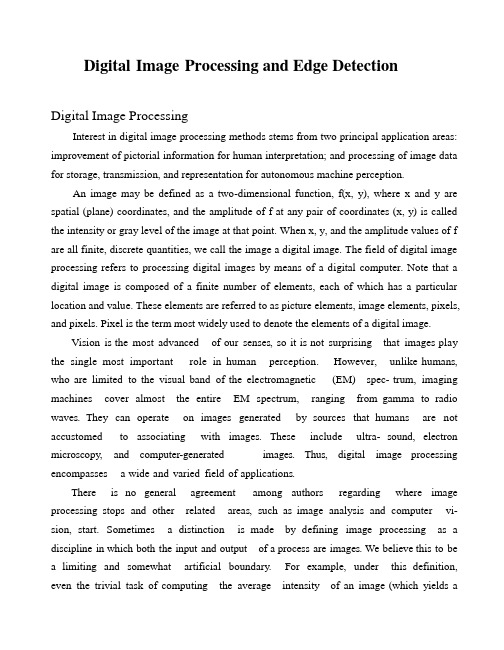
Digital Image Processing and Edge DetectionDigital Image ProcessingInterest in digital image processing methods stems from two principal application areas: improvement of pictorial information for human interpretation; and processing of image data for storage, transmission, and representation for autonomous machine perception.An image may be defined as a two-dimensional function, f(x, y), where x and y are spatial (plane) coordinates, and the amplitude of f at any pair of coordinates (x, y) is called the intensity or gray level of the image at that point. When x, y, and the amplitude values of f are all finite, discrete quantities, we call the image a digital image. The field of digital image processing refers to processing digital images by means of a digital computer. Note that a digital image is composed of a finite number of elements, each of which has a particular location and value. These elements are referred to as picture elements, image elements, pixels, and pixels. Pixel is the term most widely used to denote the elements of a digital image.Vision is the most advanced of our senses, so it is not surprising that images play the single most important role in human perception. However, unlike humans, who are limited to the visual band of the electromagnetic (EM) spec- trum, imaging machines cover almost the entire EM spectrum, ranging from gamma to radio waves. They can operate on images generated by sources that humans are not accustomed to associating with images. These include ultra- sound, electron microscopy, and computer-generated images. Thus, digital image processing encompasses a wide and varied field of applications.There is no general agreement among authors regarding where image processing stops and other related areas, such as image analysis and computer vi- sion, start. Sometimes a distinction is made by defining image processing as a discipline in which both the input and output of a process are images. We believe this to be a limiting and somewhat artificial boundary. For example, under this definition, even the trivial task of computing the average intensity of an image (which yields asingle number) would not be considered an image processing operation. On the other hand, there are fields such as computer vision whose ultimate goal is to use computers to emulate human vision, including learning and being able to make inferences and take actions based on visual inputs. This area itself is a branch of artificial intelligence (AI) whose objective is to emulate human intelligence. The field of AI is in its earliest stages of infancy in terms of development, with progress having been much slower than originally anticipated. The area of image analysis (also called image understanding) is in be- tween image processing and computer vision.There are no clearcut boundaries in the continuum from image processing at one end to computer vision at the other. However, one useful paradigm is to consider three types of computerized processes in this continuum: low-, mid-, and high level processes. Low-level processes involve primitive opera- tions such as image preprocessing to reduce noise, contrast enhancement, and image sharpening. A low-level process is characterized by the fact that both its inputs and outputs are images. Mid-level processing on images involves tasks such as segmentation (partitioning an image into regions or objects), description of those objects to reduce them to a form suitable for computer processing, and classification (recognition) of individual objects. A midlevel process is characterized by the fact that its inputs generally are images, but its outputs are attributes extracted from those images (e.g., edges, contours, and the identity of individual objects). Finally, higher level processing involves “making sense” of an ensemble of recognized objects, as in image analysis, and, at the far end of the continuum, performing the cognitive functions normally associated with vision.Based on the preceding comments, we see that a logical place of overlap between image processing and image analysis is the area of recognition of individual regions or objects in an image. Thus, what we call in this book digital image processing encompasses processes whose inputs and outputs are images and, in addition, encompasses processes that extract attributes from images, up to and including the recognition of individual objects. As a simple illustration to clarify these concepts, consider the area of automated analysis of text. The processes of acquiring an image of the area containing the text, preprocessing that image, extracting(segmenting) the individual characters, describing the characters in a form suitable for computer processing, and recognizing those individual characters are in the scope of what we call digital image processing in this book. Making sense of the content of the page may be viewed as being in the domain of image analysis and even computer vision, depending on the level of complexity implied by the statement “making sense.”As will become evident shortly, digital image processing, as we have defined it, is used successfully in a broad range of areas of exceptional social and economic value.The areas of application of digital image processing are so varied that some form of organization is desirable in attempting to capture the breadth of this field. One of the simplest ways to develop a basic understanding of the extent of image processing applications is to categorize images according to their source (e.g., visual, X-ray, and so on). The principal energy source for images in use today is the electromagnetic energy spectrum. Other important sources of energy include acoustic, ultrasonic, and electronic (in the form of electron beams used in electron microscopy). Synthetic images, used for modeling and visualization, are generated by computer. In this section we discuss briefly how images are generated in these various categories and the areas in which they are applied.Images based on radiation from the EM spectrum are the most familiar, especially images in the X-ray and visual bands of the spectrum. Electromagnet- ic waves can be conceptualized as propagating sinusoidal waves of varying wavelengths, or they can be thought of as a stream of massless particles, each traveling in a wavelike pattern and moving at the speed of light. Each massless particle contains a certain amount (or bundle) of energy. Each bundle of energy is called a photon. If spectral bands are grouped according to energy per photon, we obtain the spectrum shown in fig. below, ranging from gamma rays (highest energy) at one end to radio waves (lowest energy) at the other. The bands are shown shaded to convey the fact that bands of the EM spectrum are not distinct but rather transition smoothly from one to theother.Image acquisition is the first process. Note that acquisition could be as simple as being given an image that is already in digital form. Generally, the image acquisition stage involves preprocessing, such as scaling.Image enhancement is among the simplest and most appealing areas of digital image processing. Basically, the idea behind enhancement techniques is to bring out detail that is obscured, or simply to highlight certain features of interest in an image. A familiar example of enhancement is when we increase the contrast of an image because “it looks better.” It is important to keep in mind that enhancement is a very subjective area of image processing. Image restoration is an area that also deals with improving the appearance of an image. However, unlike enhancement, which is subjective, image restoration is objective, in the sense that restoration techniques tend to be based on mathematical or probabilistic models of image degradation. Enhancement, on the other hand, is based on human subjective preferences regarding what constitutes a “good”enhancement result.Color image processing is an area that has been gaining in importance because of the significant increase in the use of digital images over the Internet. It covers a number of fundamental concepts in color models and basic color processing in a digital domain. Color is used also in later chapters as the basis for extracting features of interest in an image.Wavelets are the foundation for representing images in various degrees of resolution. In particular, this material is used in this book for image data compression and for pyramidal representation, in which images are subdivided successively into smaller regions.Compression, as the name implies, deals with techniques for reducing the storage required to save an image, or the bandwidth required to transmit it.Although storage technology has improved significantly over the past decade, the same cannot be said for transmission capacity. This is true particularly in uses of the Internet, which are characterized by significant pictorial content. Image compression is familiar (perhaps inadvertently) to most users of computers in the form of image , such as the jpg used in the JPEG (Joint Photographic Experts Group) image compression standard.Morphological processing deals with tools for extracting image components that are useful in the representation and description of shape. The material in this chapter begins a transition from processes that output images to processes that output image attributes.Segmentation procedures partition an image into its constituent parts or objects. In general, autonomous segmentation is one of the most difficult tasks in digital image processing. A rugged segmentation procedure brings the process a longway toward successful solution of imaging problems that require objects to be identified individually. On the other hand, weak or erratic segmentation algorithms almost always guarantee eventual failure. In general, the more accurate the segmentation, the more likely recognition is to succeed.Representation and description almost always follow the output of a segmentation stage, which usually is raw pixel data, constituting either the boundary of a region (i.e., the set of pixels separating one image region from another) or all the points in the region itself. In either case, converting the data to a form suitable for computer processing is necessary. The first decision that must be made is whether the data should be represented as a boundary or as a complete region. Boundary representation is appropriate when the focus is on external shape characteristics, such as corners and inflections. Regional representation is appropriate when the focus is on internal properties, such as texture or skeletal shape. In some applications, these representations complement each other. Choosing a representation is only part of the solution for trans- forming raw data into a form suitable for subsequent computer processing. A method must also be specified for describing the data so that features of interest are highlighted. Description, also called feature selection, deals with extracting attributes that result in some quantitative information of interest or are basic for differentiating one class of objects from another.Recognition is the process that assigns a label (e.g., “vehicle”) to an object based on its descriptors. As detailed before, we conclude our coverage of digital image processing with the development of methods for recognition of individual objects.So far we have said nothing about the need for prior knowledge or about the interaction between the knowledge base and the processing modules in Fig 2 above. Knowledge about a problem domain is coded into an image processing system in the form of a knowledge database. This knowledge may be as simple as detailing regions of an image where theinformation of interest is known to be located, thus limiting the search that has to be conducted in seeking that information. The knowledge base also can be quite complex, such as an interrelated list of all major possible defects in a materials inspection problem or an image database containing high-resolution satellite images of a region in connection with change-detection applications. In addition to guiding the operation of each processing module, the knowledge base also controls the interaction between modules. This distinction is made in Fig 2 above by the use of double-headed arrows between the processing modules and the knowledge base, as opposed to single-headed arrows linking the processing modules.Edge detectionEdge detection is a terminology in image processing and computer vision, particularly in the areas of feature detection and feature extraction, to refer to algorithms which aim at identifying points in a digital image at which the image brightness changes sharply or more formally has discontinuities.Although point and line detection certainly are important in any discussion on segmentation,edge detection is by far the most common approach for detecting meaningful discounties in gray level.Although certain literature has considered the detection of ideal step edges, the edges obtained from natural images are usually not at all ideal step edges. Instead they are normally affected by one or several of the following effects:1.focal blur caused by a finite depth-of-field and finite point spread function; 2.penumbral blur caused by shadows created by light sources of non-zero radius; 3.shading at a smooth object edge; 4.local specularities or interreflections in the vicinity of object edges.A typical edge might for instance be the border between a block of red color and a block of yellow. In contrast a line (as can be extracted by a ridge detector) can be a small number of pixels of a different color on an otherwise unchanging background. For a line, there maytherefore usually be one edge on each side of the line.To illustrate why edge detection is not a trivial task, let us consider the problem of detecting edges in the following one-dimensional signal. Here, we may intuitively say that there should be an edge between the 4th and 5th pixels.If the intensity difference were smaller between the 4th and the 5th pixels and if the intensity differences between the adjacent neighbouring pixels were higher, it would not be as easy to say that there should be an edge in the corresponding region. Moreover, one could argue that this case is one in which there are several edges.Hence, to firmly state a specific threshold on how large the intensity change between two neighbouring pixels must be for us to say that there should be an edge between these pixels is not always a simple problem. Indeed, this is one of the reasons why edge detection may be a non-trivial problem unless the objects in the scene are particularly simple and the illumination conditions can be well controlled.There are many methods for edge detection, but most of them can be grouped into two categories,search-based and zero-crossing based. The search-based methods detect edges by first computing a measure of edge strength, usually a first-order derivative expression such as the gradient magnitude, and then searching for local directional maxima of the gradient magnitude using a computed estimate of the local orientation of the edge, usually the gradient direction. The zero-crossing based methods search for zero crossings in a second-order derivative expression computed from the image in order to find edges, usually the zero-crossings of the Laplacian of the zero-crossings of a non-linear differential expression, as will be described in the section on differential edge detection following below. As a pre-processing step to edge detection, a smoothing stage, typically Gaussian smoothing, is almost always applied (see also noise reduction).The edge detection methods that have been published mainly differ in the types of smoothing filters that are applied and the way the measures of edge strength are computed. As many edge detection methods rely on the computation of image gradients, they also differ in the types of filters used for computing gradient estimates in the x- and y-directions.Once we have computed a measure of edge strength (typically the gradient magnitude), the next stage is to apply a threshold, to decide whether edges are present or not at an image point. The lower the threshold, the more edges will be detected, and the result will be increasingly susceptible to noise, and also to picking out irrelevant features from the image. Conversely a high threshold may miss subtle edges, or result in fragmented edges.If the edge thresholding is applied to just the gradient magnitude image, the resulting edges will in general be thick and some type of edge thinning post-processing is necessary. For edges detected with non-maximum suppression however, the edge curves are thin by definition and the edge pixels can be linked into edge polygon by an edge linking (edge tracking) procedure. On a discrete grid, the non-maximum suppression stage can be implemented by estimating the gradient direction using first-order derivatives, then rounding off the gradient direction to multiples of 45 degrees, and finally comparing the values of the gradient magnitude in the estimated gradient direction.A commonly used approach to handle the problem of appropriate thresholds for thresholding is by using thresholding with hysteresis. This method uses multiple thresholds to find edges. We begin by using the upper threshold to find the start of an edge. Once we have a start point, we then trace the path of the edge through the image pixel by pixel, marking an edge whenever we are above the lower threshold. We stop marking our edge only when the value falls below our lower threshold. This approach makes the assumption that edges are likely to be in continuous curves, and allows us to follow a faint section of an edge we have previously seen, without meaning that every noisy pixel in the image is marked down as an edge. Still, however, we have the problem of choosing appropriate thresholdingparameters, and suitable thresholding values may vary over the image.Some edge-detection operators are instead based upon second-order derivatives of the intensity. This essentially captures the rate of change in the intensity gradient. Thus, in the ideal continuous case, detection of zero-crossings in the second derivative captures local maxima in the gradient.We can come to a conclusion that,to be classified as a meaningful edge point,the transition in gray level associated with that point has to be significantly stronger than the background at that point.Since we are dealing with local computations,the method of choice to determine whether a value is “significant” or not id to use a threshold.Thus we define a point in an image as being as being an edge point if its two-dimensional first-order derivative is greater than a specified criterion of connectedness is by definition an edge.The term edge segment generally is used if the edge is short in relation to the dimensions of the image.A key problem in segmentation is to assemble edge segments into longer edges.An alternate definition if we elect to use the second-derivative is simply to define the edge ponits in an image as the zero crossings of its second derivative.The definition of an edge in this case is the same as above.It is important to note that these definitions do not guarantee success in finding edge in an image.They simply give us a formalism to look for them.First-order derivatives in an image are computed using the gradient.Second-order derivatives are obtained using the Laplacian.数字图像处理和边缘检测数字图像处理在数字图象处理方法的兴趣从两个主要应用领域的茎:改善人类解释图像信息;和用于存储,传输,和表示用于自主机器感知图像数据的处理。
- 1、下载文档前请自行甄别文档内容的完整性,平台不提供额外的编辑、内容补充、找答案等附加服务。
- 2、"仅部分预览"的文档,不可在线预览部分如存在完整性等问题,可反馈申请退款(可完整预览的文档不适用该条件!)。
- 3、如文档侵犯您的权益,请联系客服反馈,我们会尽快为您处理(人工客服工作时间:9:00-18:30)。
Equalization: Discrete Case
Equalization: Discrete Case
直方图调整法
(二)直方图匹配 修改一幅图象的直方图,使得 它与另一幅图象的直方图匹配或 具有一种预先规定的函数形状。 目标:突出我们感兴趣的灰度 范围,使图象质量改善。
连续灰度的直方图原图
对角邻域
8邻域
2.5 像素间的一些基本关系
像素的连通性 -- 像素的连通性能够帮助简化区域、边界等概念; -- 确定两个像素是否连通,看它们是否相邻以及灰度值是否满足特定的相 似性准则。
定义V是用于定义邻接性的灰度值集合,存在三种类型的邻接性: (1)4邻接:如果q在N4(p)集中,具有V中数值的两个像素p和q是4邻接的. (2)8邻接:如果q在N8(p)集中,具有V中数值的两个像素p和q是8邻接的. (3)m邻接(混合邻接):如果(i)q在N4(p)中,或者(ii)q在ND(p)中且集合
rk r0=0 r1=1/7 r2=2/7 r3=3/7 r4=4/7 r5=5/7 r6=6/7 r7=1
nk 790 1023 850 656 329 245 122 81
p(rk) 0.19 0.25 0.21 0.16 0.08 0.06 0.03 0.02
sk计算 0.19 0.44 0.65 0.81 0.89 0.95 0.98 1.00
[0 255] [0 65535] [0 16.2*106]
1 byte, very common common in research common in color (i.e. 3*8 for RGB)
Common quantization levels
2.5 像素间的一些基本关系
像素p,坐标(x,y)的邻居
连续灰度的直方图规定
直方图匹配
令P(r) 为原始图象的灰度密度函 数,P(z)是期望通过匹配的图象灰 度密度函数。对P(r) 及P(z) 作直方 图均衡变换,通过直方图均衡为 桥梁,实现P(r) 与P(z) 变换。
直 方 图 匹 配
变 换 公 式 推 导 图 示
zk rj
直方图匹配
步骤: (1)由
2.1 视觉感知要素
眼睛的构造: (人眼包含有三层膜)
眼角膜与巩膜外壳 脉络膜 (前面睫状体 虹膜 晶状体) 视网膜 (视网膜表面的分离光
接收器提供图案视觉, 分为锥状体、杆状体)
锥状体:位于视网膜中间,对颜色 灵敏度高,分辨图像细节. 白昼视觉 杆状体:分布在视网膜表面,无彩 色感觉,在低照明度下对 图像较敏感,用来给出 视野内一般的总体图像. 夜视觉
2.5 像素间的一些基本关系
距离度量: 对于像素p,q和z,其坐标分别为(x,y),(s,t)和(v,w),如果: (a) D(p,q)≥0 [D(p,q)=0,当且仅当p=q] (b) D(p,q)=D(q,p) (c) D(p,z)≤D(p,q)+D(q,z) 则D是距离函数或度量. 欧式距离:De(p,q)=[(x-s)2+(y-t)2]1/2 (距离小于等于r的像素形成中心在(x,y)的圆) D4距离:D4(p,q)=|x-s|+|y-t| (距离小于等于r的像素形成中心在(x,y)的菱形) D8距离:D8(p,q)=max(|x-s|,|y-t|) (距离小于等于r的像素形成中心在(x,y)的方形)
Imaging System
Imaged Object
End User
Radiation or Energy Image Formation
Display
Spectroscopy
Detection
Processing
Fundamental Steps
Components of an Image Processing Systems
2.5 像素间的一些基本关系
相邻像素
对于像素p,坐标(x,y)
4邻域 (x+1,y),(x-1,y),(x,y+1),(x,y-1) N4(p) 对角邻域 (x+1,y+1),(x+1,y-1),(x-1,y+1),(x-1,y-1) ND(p) 8邻域 N4(p) + ND(p) N8(p)
4邻域
例
2. 把计算的sk就近安排到8个 灰度级中。
rk r0=0 r1=1/7 r2=2/7 r3=3/7 r4=4/7 r5=5/7 r6=6/7 r7=1
nk 790 1023 850 656 329 245 122 81
p(rk) 0.19 0.25 0.21 0.16 0.08 0.06 0.03 0.02
Components of an Image Processing Systems
world
Imaging Visualisation
Image Processing
Image Analysis
data
Computer Graphics
image
“knowledge”
Image understanding Computer vision
可以定义4邻接,8邻接和m邻接
2.5 像素间的一些基本关系
像素p (x,y)到像素q (s,t)的通路(path): 特定的像素序列(x0,y0),(x1,y1),…,(xn,yn),其中(x0,y0)=(x,y), (xn,yn)=(s,t),且像素(xi,yi)和(xi-1,yi-1)(对于1≤i≤n)是邻接的. n是通路的长度.若(x0,y0)=(xn,yn),则通路是闭合通路.
Equalization: Discrete Case
Equalization: Discrete Case
Histograms Equalization
Histograms Equalization
Histograms Equalization
Histograms Equalization
sk s0 s1 s2 s3
nsk p(sk) 790 0.19 1023 0.25 850 0.21 985 0.24
s4 44均衡化
直方图均衡化
直方图均衡化实质上是减少图象的 灰度级以换取对比度的加大。在均衡 过程中,原来的直方图上频数较小的 灰度级被归入很少几个或一个灰度级 内,故得不到增强。若这些灰度级所 构成的图象细节比较重要,则需采用 局部区域直方图均衡。
直方图均衡化变换公式推导图示
sj+s sj
rj
rj+r
直方图均衡化
考虑到灰度变换不影响象素的位 置分布,也不会增减象素数目。所 以有
r
0
p(r )dr p( s)ds 1 ds s T (r )
0 0
s
s
T (r ) p(r )dr
0
r
(2 1)
算例
直方图均衡化
应用到离散灰度级,设一幅图象的 象素总数为n,分L个灰度级。 nk: 第k个灰度级出现的频数。 第k个灰度级出现的概率 P(rk)=nk/n 其中0≤rk≤1,k=0,1,2,...,L-1 形式为:
sk T (rk ) p(rj )
j 0 j 0 k k
nj n
Brightness Adaptation
人眼对不同亮度的适应和鉴别能力
亮度适应范围: 1010量级 10-6ml 到 104ml 实验表明,主观亮度是进入 眼睛亮度的对数函数 亮度适应现象:
人眼并不能同时在整个范围内 工作,而是利用改变整个灵敏 度来完成这一大变动的.
亮度适应级:视觉系统当前 的灵敏度级别
2.5 像素间的一些基本关系
1.4 1 1.4 1 0 1 1.4 1 1.4 2 1 2 1 0 1 2 1 2 1 1 1 1 0 1 1 1 1
2.5 像素间的一些基本关系
基于像素的图像操作
2.6
线性和非线性操作
令H是一种算子,其输入和输出都是图像,如果对于任何两幅图像f和g 及其任何两个标量a和b有如下关系,则称H为线性算子: H(af+bg)=aH(f)+bH(g)
s T (r ) p(r )dr
0
r
0 r 1
8通路
m通路
2.5 像素间的一些基本关系
像素p (x,y)到像素q (s,t)的连通: 令S表示一幅图像中的像素子集,如果在S中全部像素之间存在一个通路, 则可以说两个像素p和q在S中是连通的. 对于S中的任何像素p,S中连通到该像素的像素集叫做S的连通分量.如果S 仅有一个连通分量,则集合S叫做连通集. 令R是图像中的像素子集.如果R是连通集,则称R为一个区域. 一个区域R的边界(也称为边缘或轮廓)是区域中像素的集合,该区域 有一个或多个不在R中的邻点. 如果R是整幅图像,则边界由图像第一行、第一列和最后一行一列定义. 正常情况下,区域指一幅图像的子集,并包括区域的边缘.
(2 2)
例
例:设图象有64*64=4096个象素,有8个灰度级,灰度 分布如表所示。进行直方图均衡化。
rk r0=0 r1=1/7 r2=2/7 r3=3/7 r4=4/7 r5=5/7 r6=6/7 r7=1
nk 790 1023 850 656 329 245 122 81
p(rk) 0.19 0.25 0.21 0.16 0.08 0.06 0.03 0.02
直方图均衡化
首先假定连续灰度级的情况,推导 直方图均衡化变换公式,令 r 代表灰 度级, P ( r ) 为概率密度函数。 r值已归一化,最大灰度值为1。
连续灰度的直方图非均匀分布
连续灰度的直方图均匀分布
直方图均衡化目标
直方图均衡化
直方图均衡化
要找到一种变换 S=T ( r ) 使直方图变平直, 为使变换后的灰度仍保持从黑到白的单一变 化顺序,且变换范围与原先一致,以避免整 体变亮或变暗。必须规定: (1)在0≤r≤1中,T(r)是单调递增函数, 且0≤T(r)≤1; (2)反变换r=T-1(s),T-1(s)也为单调递增函 数,0≤s≤1。