计量经济学第13节习题答案Word版
计量经济学(数字教材版)课后习题参考答案
课后习题参考答案第二章教材习题与解析1、 判断下列表达式是否正确:y i =β0+β1x i ,i =1,2,⋯ny ̂i =β̂0+β̂1x i ,i =1,2,⋯nE(y i |x i )=β0+β1x i +u i ,i =1,2,⋯n E(y i |x i )=β0+β1x i ,i =1,2,⋯nE(y i |x i )=β̂0+β̂1x i ,i =1,2,⋯ny i =β0+β1x i +u i ,i =1,2,⋯ny ̂i =β̂0+β̂1x i +u i ,i =1,2,⋯n y i =β̂0+β̂1x i +u i ,i =1,2,⋯n y i =β̂0+β̂1x i +u ̂i ,i =1,2,⋯n y ̂i =β̂0+β̂1x i +u ̂i ,i =1,2,⋯n答案:对于计量经济学模型有两种类型,一是总体回归模型,另一是样本回归模型。
两类回归模型都具有确定形式与随机形式两种表达方式:总体回归模型的确定形式:X X Y E 10)|(ββ+= 总体回归模型的随机形式:μββ++=X Y 10样本回归模型的确定形式:X Y 10ˆˆˆββ+= 样本回归模型的随机形式:e X Y ++=10ˆˆββ 除此之外,其他的表达形式均是错误的2、给定一元线性回归模型:y =β0+β1x +u (1)叙述模型的基本假定;(2)写出参数β0和β1的最小二乘估计公式;(3)说明满足基本假定的最小二乘估计量的统计性质; (4)写出随机扰动项方差的无偏估计公式。
答案:(1)线性回归模型的基本假设有两大类,一类是关于随机误差项的,包括零均值、同方差、不序列相关、满足正态分布等假设;另一类是关于解释变量的,主要是解释变量是非随机的,如果是随机变量,则与随机误差项不相关。
(2)12ˆi iix yxβ=∑∑,01ˆˆY X ββ=- (3)考察总体的估计量,可从如下几个方面考察其优劣性:1)线性性,即它是否是另一个随机变量的线性函数; 2)无偏性,即它的均值或期望是否等于总体的真实值;3)有效值,即它是否在所有线性无偏估计量中具有最小方差;4)渐进无偏性,即样本容量趋于无穷大时,它的均值序列是否趋于总体真值; 5)一致性,即样本容量趋于无穷大时,它是否依概率收敛于总体的真值;6)渐进有效性,即样本容量趋于无穷大时,它在所有的一致估计量中是否具有最小的渐进方差。
计量经济学习题及参考答案解析详细版

计量经济学习题及参考答案解析详细版计量经济学(第四版)习题参考答案潘省初第⼀章绪论试列出计量经济分析的主要步骤。
⼀般说来,计量经济分析按照以下步骤进⾏:(1)陈述理论(或假说)(2)建⽴计量经济模型(3)收集数据(4)估计参数(5)假设检验(6)预测和政策分析计量经济模型中为何要包括扰动项?为了使模型更现实,我们有必要在模型中引进扰动项u 来代表所有影响因变量的其它因素,这些因素包括相对⽽⾔不重要因⽽未被引⼊模型的变量,以及纯粹的随机因素。
什么是时间序列和横截⾯数据? 试举例说明⼆者的区别。
时间序列数据是按时间周期(即按固定的时间间隔)收集的数据,如年度或季度的国民⽣产总值、就业、货币供给、财政⾚字或某⼈⼀⽣中每年的收⼊都是时间序列的例⼦。
横截⾯数据是在同⼀时点收集的不同个体(如个⼈、公司、国家等)的数据。
如⼈⼝普查数据、世界各国2000年国民⽣产总值、全班学⽣计量经济学成绩等都是横截⾯数据的例⼦。
估计量和估计值有何区别?估计量是指⼀个公式或⽅法,它告诉⼈们怎样⽤⼿中样本所提供的信息去估计总体参数。
在⼀项应⽤中,依据估计量算出的⼀个具体的数值,称为估计值。
如Y就是⼀个估计量,1nii YY n==∑。
现有⼀样本,共4个数,100,104,96,130,则根据这个样本的数据运⽤均值估计量得出的均值估计值为5.107413096104100=+++。
第⼆章计量经济分析的统计学基础略,参考教材。
请⽤例中的数据求北京男⽣平均⾝⾼的99%置信区间NS S x ==45= ⽤也就是说,根据样本,我们有99%的把握说,北京男⾼中⽣的平均⾝⾼在⾄厘⽶之间。
25个雇员的随机样本的平均周薪为130元,试问此样本是否取⾃⼀个均值为120元、标准差为10元的正态总体?原假设120:0=µH备择假设 120:1≠µH 检验统计量()10/2510/25XX µσ-Z ====查表96.1025.0=Z 因为Z= 5 >96.1025.0=Z ,故拒绝原假设, 即此样本不是取⾃⼀个均值为120元、标准差为10元的正态总体。
计量经济学习题及全部答案
计量经济学习题及全部答案《计量经济学》习题(⼀)⼀、判断正误1.在研究经济变量之间的⾮确定性关系时,回归分析是唯⼀可⽤的分析⽅法。
() 2.最⼩⼆乘法进⾏参数估计的基本原理是使残差平⽅和最⼩。
()3.⽆论回归模型中包括多少个解释变量,总离差平⽅和的⾃由度总为(n -1)。
() 4.当我们说估计的回归系数在统计上是显著的,意思是说它显著地异于0。
() 5.总离差平⽅和(TSS )可分解为残差平⽅和(ESS )与回归平⽅和(RSS )之和,其中残差平⽅和(ESS )表⽰总离差平⽅和中可由样本回归直线解释的部分。
() 6.多元线性回归模型的F 检验和t 检验是⼀致的。
()7.当存在严重的多重共线性时,普通最⼩⼆乘估计往往会低估参数估计量的⽅差。
() 8.如果随机误差项的⽅差随解释变量变化⽽变化,则线性回归模型存在随机误差项的⾃相关。
()9.在存在异⽅差的情况下,会对回归模型的正确建⽴和统计推断带来严重后果。
() 10...DW 检验只能检验⼀阶⾃相关。
()⼆、单选题1.样本回归函数(⽅程)的表达式为()。
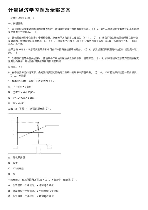
A .i Y =01i i X u ββ++B .(/)i E Y X =01i X ββ+C .i Y =01??i i X e ββ++D .?i Y =01??iX ββ+ 2.下图中“{”所指的距离是()。
A .随机⼲扰项B .残差C .i Y 的离差D .?iY 的离差 3.在总体回归⽅程(/)E Y X =01X ββ+中,1β表⽰()。
A .当X 增加⼀个单位时,Y 增加1β个单位B .当X 增加⼀个单位时,Y 平均增加1β个单位C .当Y 增加⼀个单位时,X 增加1β个单位D .当Y 增加⼀个单位时,X 平均增加1β个单位 4.可决系数2R 是指()。
A .剩余平⽅和占总离差平⽅和的⽐重B .总离差平⽅和占回归平⽅和的⽐重C .回归平⽅和占总离差平⽅和的⽐重D .回归平⽅和占剩余平⽅和的⽐重 5.已知含有截距项的三元线性回归模型估计的残差平⽅和为2i e ∑=800,估计⽤的样本容量为24,则随机误差项i u 的⽅差估计量为()。
计量经济学第二版课后习题1-14章中文版答案汇总
第四章习题 1.(1)22ˆ=TSR estScore T =520.4-5.82×22=392.36 (2)ΔTestScore=-5.82×(23-19)=-23.28即平均测试成绩所减少的分数回归预测值为23.28。
(3)core est S T =βˆ0 +βˆ1×CS =520.4-5.82×1.4=395.85 (4)SER 2=∑=-n i u n 1ˆ21i 2=11.5 ∴SSR=∑=ni u1ˆi2=SER 2×(n-2)=11.5×(100-2)=12960.5R 2=T SS ESS =1-T SSSSR =0.08∴TSS=SSR ÷(1-R 2)=12960.5÷(1-0.08)=14087.5=21)(Y ∑=-ni iY∴s Y 2=1-n 121)(Y ∑=-ni iY =14087.5÷(100-1)≈140.30∴s Y ≈11.93 2. (1)①70ˆ=Height eight W =-99.41+3.94×70=176.39 ②65ˆ=Height eight W =-99.41+3.94×65=156.69 ③74ˆ=Height eight W=-99.41+3.94×74=192.15(2)ΔWeight=3.94×1.5=5.91(3)1inch=2.54cm,1lb=0.4536kg①eight Wˆ(kg)=-99.41×0.4536+54.24536.0×94.3Height(cm)=-45.092+0.7036×Height(cm)②R 2无量纲,与计量单位无关,所以仍为0.81③SER=10.2×0.4536=4.6267kg 3.(1)①系数696.7为回归截距,决定回归线的总体水平②系数9.6为回归系数,体现年龄对周收入的影响程度,每增加1岁周收入平均增加$9.6 (2)SER=624.1美元,其度量单位为美元。
计量经济学习题集及详解答案

第一章绪论一、填空题:1.计量经济学是以揭示经济活动中客观存在的为内容的分支学科,挪威经济学家弗里希,将计量经济学定义为、、三者的结合。
2.数理经济模型揭示经济活动中各个因素之间的关系,用性的数学方程加以描述,计量经济模型揭示经济活动中各因素之间的关系,用性的数学方程加以描述。
3.经济数学模型是用描述经济活动。
4.计量经济学根据研究对象和内容侧重面不同,可以分为计量经济学和计量经济学。
5.计量经济学模型包括和两大类。
6.建模过程中理论模型的设计主要包括三部分工作,即、、。
7.确定理论模型中所包含的变量,主要指确定。
8.可以作为解释变量的几类变量有变量、变量、变量和变量。
9.选择模型数学形式的主要依据是。
10.研究经济问题时,一般要处理三种类型的数据:数据、数据和数据。
11.样本数据的质量包括四个方面、、、。
12.模型参数的估计包括、和软件的应用等内容。
13.计量经济学模型用于预测前必须通过的检验分别是检验、检验、检验和检验。
14.计量经济模型的计量经济检验通常包括随机误差项的检验、检验、解释变量的检验。
15.计量经济学模型的应用可以概括为四个方面,即、、、。
16.结构分析所采用的主要方法是、和。
二、单选题:1.计量经济学是一门()学科。
A.数学B.经济C.统计D.测量2.狭义计量经济模型是指()。
A.投入产出模型B.数学规划模型C.包含随机方程的经济数学模型D.模糊数学模型3.计量经济模型分为单方程模型和()。
A.随机方程模型B.行为方程模型C.联立方程模型D.非随机方程模型4.经济计量分析的工作程序()A.设定模型,检验模型,估计模型,改进模型B.设定模型,估计参数,检验模型,应用模型C.估计模型,应用模型,检验模型,改进模型D.搜集资料,设定模型,估计参数,应用模型5.同一统计指标按时间顺序记录的数据列称为()A.横截面数据B.时间序列数据C.修匀数据D.平行数据6.样本数据的质量问题,可以概括为完整性、准确性、可比性和()。
计量经济学习题及全部答案

计量经济学习题及全部答案计量经济学习题及全部答案标准化⼯作室编码[XX968T-XX89628-XJ668-XT689N]《计量经济学》习题(⼀)⼀、判断正误1.在研究经济变量之间的⾮确定性关系时,回归分析是唯⼀可⽤的分析⽅法。
()2.最⼩⼆乘法进⾏参数估计的基本原理是使残差平⽅和最⼩。
()3.⽆论回归模型中包括多少个解释变量,总离差平⽅和的⾃由度总为(n -1)。
()4.当我们说估计的回归系数在统计上是显着的,意思是说它显着地异于0。
()5.总离差平⽅和(TSS )可分解为残差平⽅和(ESS )与回归平⽅和(RSS )之和,其中残差平⽅和(ESS )表⽰总离差平⽅和中可由样本回归直线解释的部分。
()6.多元线性回归模型的F 检验和t 检验是⼀致的。
()7.当存在严重的多重共线性时,普通最⼩⼆乘估计往往会低估参数估计量的⽅差。
()8.如果随机误差项的⽅差随解释变量变化⽽变化,则线性回归模型存在随机误差项的⾃相关。
()9.在存在异⽅差的情况下,会对回归模型的正确建⽴和统计推断带来严重后果。
()10...DW 检验只能检验⼀阶⾃相关。
()⼆、单选题1.样本回归函数(⽅程)的表达式为()。
A .i Y =01i i X u ββ++B .(/)i E Y X =01i X ββ+C .i Y =01??i i X e ββ++D .?i Y =01??iX ββ+ 2A .随机⼲扰项B .残差C .i Y 的离差D .?iY 的离差 3.在总体回归⽅程(/)E Y X =01X ββ+中,1β表⽰()。
A .当X 增加⼀个单位时,Y 增加1β个单位B .当X 增加⼀个单位时,Y 平均增加1β个单位C .当Y 增加⼀个单位时,X 增加1β个单位D .当Y 增加⼀个单位时,X 平均增加1β个单位4.可决系数2R 是指()。
A .剩余平⽅和占总离差平⽅和的⽐重B .总离差平⽅和占回归平⽅和的⽐重C .回归平⽅和占总离差平⽅和的⽐重D .回归平⽅和占剩余平⽅和的⽐重5.已知含有截距项的三元线性回归模型估计的残差平⽅和为2i e ∑=800,估计⽤的样本容量为24,则随机误差项i u 的⽅差估计量为()。
(完整word版)计量经济学基本点练习题及答案
(完整word版)计量经济学基本点练习题及答案Chap1—31、在同⼀时间不同统计单位的相同统计指标组成的数据组合,是()A、原始数据B、时点数据C、时间序列数据D、截⾯数据2、回归分析中定义的( )A、解释变量和被解释变量都是随机变量B、解释变量为⾮随机变量,被解释变量为随机变量C、解释变量和被解释变量都为⾮随机变量D、解释变量为随机变量,被解释变量为⾮随机变量3、在⼀元线性回归模型中,样本回归⽅程可表⽰为:()4、⽤模型描述现实经济系统的原则是( )A、以理论分析作先导,解释变量应包括所有解释变量B、以理论分析作先导,模型规模⼤⼩要适度C、模型规模越⼤越好;这样更切合实际情况D、模型规模⼤⼩要适度,结构尽可能复杂5、回归分析中使⽤的距离是点到直线的垂直坐标距离。
最⼩⼆乘准则是指()6、设OLS法得到的样本回归直线为A、⼀定不在回归直线上B、⼀定在回归直线上C、不⼀定在回归直线上D、在回归直线上⽅7、下图中“{”所指的距离是A.随机误差项B.残差C.因变量观测值的离差D.因变量估计值的离差8、下⾯哪⼀个必定是错误的9、线性回归模型的OLS估计量是随机变量Y的函数,所以OLS估计量是()。
A.随机变量B.⾮随机变量C.确定性变量D.常量10、为了对回归模型中的参数进⾏假设检验,必须在古典线性回归模型基本假定之外,再增加以下哪⼀个假定:A.解释变量与随机误差项不相关B.随机误差项服从正态分布C.随机误差项的⽅差为常数D.两个误差项之间不相关D B C B D B B C A BChap41、⽤OLS估计总体回归模型,以下说法不正确的是:2、包含有截距项的⼆元线性回归模型中的回归平⽅和ESS的⾃由度是()A、nB、n-2C、n-3D、23、对多元线性回归⽅程的显著性检验,,k代表回归模型中待估参数的个数,所⽤的F统计量可表⽰为:4、已知三元线性回归模型估计的残差平⽅和为800,样本容量为24,则随机误差项的⽅差估计量为( )A 、33.33B 、 40C 、 38.09D 、36.365、在多元回归中,调整后的判定系数与判定系数的关系为6、下⾯哪⼀表述是正确的:A.线性回归模型的零均值假设是指B.对模型进⾏⽅程总体显著性检验(即F 检验),检验的零假设是C.相关系数较⼤意味着两个变量存在较强的因果关系D.当随机误差项的⽅差估计量等于零时,说明被解释变量与解释变量之间为函数关系7、在模型的回归分析结果报告中,有F=263489,p=0.000,则表明()A 、解释变量X1对Y 的影响是显著的B 、解释变量X2对Y 的影响是显著的C 、解释变量X1, X2对的Y 联合影响是显著的D 、解释变量X1, X2对的Y 的影响是均不显著8、关于判定系数,以下说法中错误的是()A 、判定系数是因变量的总变异中能由回归⽅程解释的⽐例;B 、判定系数的取值范围为0到1;C 、判定系数反映了样本回归线对样本观测值拟合优劣程度的⼀种描述;D 、判定系数的⼤⼩不受到回归模型中所包含的解释变量个数的影响。
计量经济学导论CH13习题答案
CHAPTER 13TEACHING NOTESWhile this chapter falls under “Advanced Topics,” most of this chapter requires no more sophistication than the previous chapters. (In fact, I would argue that, with the possible exception of Section 13.5, this material is easier than some of the time series chapters.)Pooling two or more independent cross sections is a straightforward extension of cross-sectional methods. Nothing new needs to be done in stating assumptions, except possibly mentioning that random sampling in each time period is sufficient. The practically important issue is allowing for different intercepts, and possibly different slopes, across time.The natural experiment material and extensions of the difference-in-differences estimator is widely applicable and, with the aid of the examples, easy to understand.Two years of panel data are often available, in which case differencing across time is a simple way of removing g unobserved heterogeneity. If you have covered Chapter 9, you might compare this with a regression in levels using the second year of data, but where a lagged dependent variable is included. (The second approach only requires collecting information on the dependent variable in a previous year.) These often give similar answers. Two years of panel data, collected before and after a policy change, can be very powerful for policy analysis. Having more than two periods of panel data causes slight complications in that the errors in the differenced equation may be serially correlated. (However, the traditional assumption that the errors in the original equation are serially uncorrelated is not always a good one. In other words, it is not always more appropriate to used fixed effects, as in Chapter 14, than first differencing.) With large N and relatively small T, a simple way to account for possible serial correlation after differencing is to compute standard errors that are robust to arbitrary serial correlation and heteroskedasticity. Econometrics packages that do cluster analysis (such as Stata) often allow this by specifying each cross-sectional unit as its own cluster.108SOLUTIONS TO PROBLEMS13.1 Without changes in the averages of any explanatory variables, the average fertility rate fellby .545 between 1972 and 1984; this is simply the coefficient on y84. To account for theincrease in average education levels, we obtain an additional effect: –.128(13.3 – 12.2) ≈–.141. So the drop in average fertility if the average education level increased by 1.1 is .545+ .141 = .686, or roughly two-thirds of a child per woman.13.2 The first equation omits the 1981 year dummy variable, y81, and so does not allow anyappreciation in nominal housing prices over the three year period in the absence of an incinerator. The interaction term in this case is simply picking up the fact that even homes that are near the incinerator site have appreciated in value over the three years. This equation suffers from omitted variable bias.The second equation omits the dummy variable for being near the incinerator site, nearinc,which means it does not allow for systematic differences in homes near and far from the sitebefore the site was built. If, as seems to be the case, the incinerator was located closer to lessvaluable homes, then omitting nearinc attributes lower housing prices too much to theincinerator effect. Again, we have an omitted variable problem. This is why equation (13.9) (or,even better, the equation that adds a full set of controls), is preferred.13.3 We do not have repeated observations on the same cross-sectional units in each time period,and so it makes no sense to look for pairs to difference. For example, in Example 13.1, it is veryunlikely that the same woman appears in more than one year, as new random samples areobtained in each year. In Example 13.3, some houses may appear in the sample for both 1978and 1981, but the overlap is usually too small to do a true panel data analysis.β, but only13.4 The sign of β1 does not affect the direction of bias in the OLS estimator of1whether we underestimate or overestimate the effect of interest. If we write ∆crmrte i = δ0 +β1∆unem i + ∆u i, where ∆u i and ∆unem i are negatively correlated, then there is a downward biasin the OLS estimator of β1. Because β1 > 0, we will tend to underestimate the effect of unemployment on crime.13.5 No, we cannot include age as an explanatory variable in the original model. Each person inthe panel data set is exactly two years older on January 31, 1992 than on January 31, 1990. This means that ∆age i = 2 for all i. But the equation we would estimate is of the form∆saving i = δ0 + β1∆age i +…,where δ0 is the coefficient the year dummy for 1992 in the original model. As we know, whenwe have an intercept in the model we cannot include an explanatory variable that is constant across i; this violates Assumption MLR.3. Intuitively, since age changes by the same amount for everyone, we cannot distinguish the effect of age from the aggregate time effect.10913.6 (i) Let FL be a binary variable equal to one if a person lives in Florida, and zero otherwise. Let y90 be a year dummy variable for 1990. Then, from equation (13.10), we have the linear probability modelarrest = β0 + δ0y90 + β1FL + δ1y90⋅FL + u.The effect of the law is measured by δ1, which is the change in the probability of drunk driving arrest due to the new law in Florida. Including y90 allows for aggregate trends in drunk driving arrests that would affect both states; including FL allows for systematic differences between Florida and Georgia in either drunk driving behavior or law enforcement.(ii) It could be that the populations of drivers in the two states change in different ways over time. For example, age, race, or gender distributions may have changed. The levels of education across the two states may have changed. As these factors might affect whether someone is arrested for drunk driving, it could be important to control for them. At a minimum, there is the possibility of obtaining a more precise estimator of δ1 by reducing the error variance. Essentially, any explanatory variable that affects arrest can be used for this purpose. (See Section 6.3 for discussion.)SOLUTIONS TO COMPUTER EXERCISES13.7 (i) The F statistic (with 4 and 1,111 df) is about 1.16 and p-value ≈ .328, which shows that the living environment variables are jointly insignificant.(ii) The F statistic (with 3 and 1,111 df) is about 3.01 and p-value ≈ .029, and so the region dummy variables are jointly significant at the 5% level.(iii) After obtaining the OLS residuals, ˆu, from estimating the model in Table 13.1, we run the regression 2ˆu on y74, y76, …, y84 using all 1,129 observations. The null hypothesis of homoskedasticity is H0: γ1 = 0, γ2= 0, … , γ6 = 0. So we just use the usual F statistic for joint significance of the year dummies. The R-squared is about .0153 and F ≈ 2.90; with 6 and 1,122 df, the p-value is about .0082. So there is evidence of heteroskedasticity that is a function of time at the 1% significance level. This suggests that, at a minimum, we should compute heteroskedasticity-robust standard errors, t statistics, and F statistics. We could also use weighted least squares (although the form of heteroskedasticity used here may not be sufficient; it does not depend on educ, age, and so on).(iv) Adding y74⋅educ, , y84⋅educ allows the relationship between fertility and education to be different in each year; remember, the coefficient on the interaction gets added to the coefficient on educ to get the slope for the appropriate year. When these interaction terms are added to the equation, R2≈ .137. The F statistic for joint significance (with 6 and 1,105 df) is about 1.48 with p-value ≈ .18. Thus, the interactions are not jointly significant at even the 10% level. This is a bit misleading, however. An abbreviated equation (which just shows the coefficients on the terms involving educ) is110111kids= -8.48 - .023 educ + - .056 y74⋅educ - .092 y76⋅educ(3.13) (.054) (.073) (.071) - .152 y78⋅educ - .098 y80⋅educ - .139 y82⋅educ - .176 y84⋅educ .(.075) (.070) (.068) (.070)Three of the interaction terms, y78⋅educ , y82⋅educ , and y84⋅educ are statistically significant at the 5% level against a two-sided alternative, with the p -value on the latter being about .012. The coefficients are large in magnitude as well. The coefficient on educ – which is for the base year, 1972 – is small and insignificant, suggesting little if any relationship between fertility andeducation in the early seventies. The estimates above are consistent with fertility becoming more linked to education as the years pass. The F statistic is insignificant because we are testing some insignificant coefficients along with some significant ones.13.8 (i) The coefficient on y85 is roughly the proportionate change in wage for a male (female = 0) with zero years of education (educ = 0). This is not especially useful since we are not interested in people with no education.(ii) What we want to estimate is θ0 = δ0 + 12δ1; this is the change in the intercept for a male with 12 years of education, where we also hold other factors fixed. If we write δ0 = θ0 - 12δ1, plug this into (13.1), and rearrange, we getlog(wage ) = β0 + θ0y85 + β1educ + δ1y85⋅(educ – 12) + β2exper + β3exper 2 + β4union + β5female + δ5y85⋅female + u .Therefore, we simply replace y85⋅educ with y85⋅(educ – 12), and then the coefficient andstandard error we want is on y85. These turn out to be 0ˆθ = .339 and se(0ˆθ) = .034. Roughly, the nominal increase in wage is 33.9%, and the 95% confidence interval is 33.9 ± 1.96(3.4), or about 27.2% to 40.6%. (Because the proportionate change is large, we could use equation (7.10), which implies the point estimate 40.4%; but obtaining the standard error of this estimate is harder.)(iii) Only the coefficient on y85 differs from equation (13.2). The new coefficient is about –.383 (se ≈ .124). This shows that real wages have fallen over the seven year period, although less so for the more educated. For example, the proportionate change for a male with 12 years of education is –.383 + .0185(12) = -.161, or a fall of about 16.1%. For a male with 20 years of education there has been almost no change [–.383 + .0185(20) = –.013].(iv) The R -squared when log(rwage ) is the dependent variable is .356, as compared with .426 when log(wage ) is the dependent variable. If the SSRs from the regressions are the same, but the R -squareds are not, then the total sum of squares must be different. This is the case, as the dependent variables in the two equations are different.(v) In 1978, about 30.6% of workers in the sample belonged to a union. In 1985, only about 18% belonged to a union. Therefore, over the seven-year period, there was a notable fall in union membership.(vi) When y85⋅union is added to the equation, its coefficient and standard error are about -.00040 (se ≈ .06104). This is practically very small and the t statistic is almost zero. There has been no change in the union wage premium over time.(vii) Parts (v) and (vi) are not at odds. They imply that while the economic return to union membership has not changed (assuming we think we have estimated a causal effect), the fraction of people reaping those benefits has fallen.13.9 (i) Other things equal, homes farther from the incinerator should be worth more, so δ1 > 0. If β1 > 0, then the incinerator was located farther away from more expensive homes.(ii) The estimated equation islog()price= 8.06 -.011 y81+ .317 log(dist) + .048 y81⋅log(dist)(0.51) (.805) (.052) (.082)n = 321, R2 = .396, 2R = .390.ˆδ = .048 is the expected sign, it is not statistically significant (t statistic ≈ .59).While1(iii) When we add the list of housing characteristics to the regression, the coefficient ony81⋅log(dist) becomes .062 (se = .050). So the estimated effect is larger – the elasticity of price with respect to dist is .062 after the incinerator site was chosen – but its t statistic is only 1.24. The p-value for the one-sided alternative H1: δ1 > 0 is about .108, which is close to being significant at the 10% level.13.10 (i) In addition to male and married, we add the variables head, neck, upextr, trunk, lowback, lowextr, and occdis for injury type, and manuf and construc for industry. The coefficient on afchnge⋅highearn becomes .231 (se ≈ .070), and so the estimated effect and t statistic are now larger than when we omitted the control variables. The estimate .231 implies a substantial response of durat to the change in the cap for high-earnings workers.(ii) The R-squared is about .041, which means we are explaining only a 4.1% of the variation in log(durat). This means that there are some very important factors that affect log(durat) that we are not controlling for. While this means that predicting log(durat) would be very difficultˆδ: it could still for a particular individual, it does not mean that there is anything biased about1be an unbiased estimator of the causal effect of changing the earnings cap for workers’ compensation.(iii) The estimated equation using the Michigan data is112durat= 1.413 + .097 afchnge+ .169 highearn+ .192 afchnge⋅highearn log()(0.057) (.085) (.106) (.154)n = 1,524, R2 = .012.The estimate of δ1, .192, is remarkably close to the estimate obtained for Kentucky (.191). However, the standard error for the Michigan estimate is much higher (.154 compared with .069). The estimate for Michigan is not statistically significant at even the 10% level against δ1 > 0. Even though we have over 1,500 observations, we cannot get a very precise estimate. (For Kentucky, we have over 5,600 observations.)13.11 (i) Using pooled OLS we obtainrent= -.569 + .262 d90+ .041 log(pop) + .571 log(avginc) + .0050 pctstu log()(.535) (.035) (.023) (.053) (.0010) n = 128, R2 = .861.The positive and very significant coefficient on d90 simply means that, other things in the equation fixed, nominal rents grew by over 26% over the 10 year period. The coefficient on pctstu means that a one percentage point increase in pctstu increases rent by half a percent (.5%). The t statistic of five shows that, at least based on the usual analysis, pctstu is very statistically significant.(ii) The standard errors from part (i) are not valid, unless we thing a i does not really appear in the equation. If a i is in the error term, the errors across the two time periods for each city are positively correlated, and this invalidates the usual OLS standard errors and t statistics.(iii) The equation estimated in differences islog()∆= .386 + .072 ∆log(pop) + .310 log(avginc) + .0112 ∆pctsturent(.037) (.088) (.066) (.0041)n = 64, R2 = .322.Interestingly, the effect of pctstu is over twice as large as we estimated in the pooled OLS equation. Now, a one percentage point increase in pctstu is estimated to increase rental rates by about 1.1%. Not surprisingly, we obtain a much less precise estimate when we difference (although the OLS standard errors from part (i) are likely to be much too small because of the positive serial correlation in the errors within each city). While we have differenced away a i, there may be other unobservables that change over time and are correlated with ∆pctstu.(iv) The heteroskedasticity-robust standard error on ∆pctstu is about .0028, which is actually much smaller than the usual OLS standard error. This only makes pctstu even more significant (robust t statistic ≈ 4). Note that serial correlation is no longer an issue because we have no time component in the first-differenced equation.11311413.12 (i) You may use an econometrics software package that directly tests restrictions such as H 0: β1 = β2 after estimating the unrestricted model in (13.22). But, as we have seen many times, we can simply rewrite the equation to test this using any regression software. Write the differenced equation as∆log(crime ) = δ0 + β1∆clrprc -1 + β2∆clrprc -2 + ∆u .Following the hint, we define θ1 = β1 - β2, and then write β1 = θ1 + β2. Plugging this into the differenced equation and rearranging gives∆log(crime ) = δ0 + θ1∆clrprc -1 + β2(∆clrprc -1 + ∆clrprc -2) + ∆u .Estimating this equation by OLS gives 1ˆθ= .0091, se(1ˆθ) = .0085. The t statistic for H 0: β1 = β2 is .0091/.0085 ≈ 1.07, which is not statistically significant.(ii) With β1 = β2 the equation becomes (without the i subscript)∆log(crime ) = δ0 + β1(∆clrprc -1 + ∆clrprc -2) + ∆u= δ0 + δ1[(∆clrprc -1 + ∆clrprc -2)/2] + ∆u ,where δ1 = 2β1. But (∆clrprc -1 + ∆clrprc -2)/2 = ∆avgclr .(iii) The estimated equation islog()crime ∆ = .099 - .0167 ∆avgclr(.063) (.0051)n = 53, R 2 = .175, 2R = .159.Since we did not reject the hypothesis in part (i), we would be justified in using the simplermodel with avgclr . Based on adjusted R -squared, we have a slightly worse fit with the restriction imposed. But this is a minor consideration. Ideally, we could get more data to determine whether the fairly different unconstrained estimates of β1 and β2 in equation (13.22) reveal true differences in β1 and β2.13.13 (i) Pooling across semesters and using OLS givestrmgpa = -1.75 -.058 spring+ .00170 sat- .0087 hsperc(0.35) (.048) (.00015) (.0010)+ .350 female- .254 black- .023 white- .035 frstsem(.052) (.123) (.117) (.076)- .00034 tothrs + 1.048 crsgpa- .027 season(.00073) (0.104) (.049)n = 732, R2 = .478, 2R = .470.The coefficient on season implies that, other things fixed, an athlete’s term GPA is about .027 points lower when his/her sport is in season. On a four point scale, this a modest effect (although it accumulates over four years of athletic eligibility). However, the estimate is not statistically significant (t statistic ≈-.55).(ii) The quick answer is that if omitted ability is correlated with season then, as we know form Chapters 3 and 5, OLS is biased and inconsistent. The fact that we are pooling across two semesters does not change that basic point.If we think harder, the direction of the bias is not clear, and this is where pooling across semesters plays a role. First, suppose we used only the fall term, when football is in season. Then the error term and season would be negatively correlated, which produces a downward bias in the OLS estimator of βseason. Because βseason is hypothesized to be negative, an OLS regression using only the fall data produces a downward biased estimator. [When just the fall data are used, ˆβ = -.116 (se = .084), which is in the direction of more bias.] However, if we use just the seasonspring semester, the bias is in the opposite direction because ability and season would be positive correlated (more academically able athletes are in season in the spring). In fact, using just theβ = .00089 (se = .06480), which is practically and statistically equal spring semester gives ˆseasonto zero. When we pool the two semesters we cannot, with a much more detailed analysis, determine which bias will dominate.(iii) The variables sat, hsperc, female, black, and white all drop out because they do not vary by semester. The intercept in the first-differenced equation is the intercept for the spring. We have∆= -.237 + .019 ∆frstsem+ .012 ∆tothrs+ 1.136 ∆crsgpa- .065 seasontrmgpa(.206) (.069) (.014) (0.119) (.043) n = 366, R2 = .208, 2R = .199.Interestingly, the in-season effect is larger now: term GPA is estimated to be about .065 points lower in a semester that the sport is in-season. The t statistic is about –1.51, which gives a one-sided p-value of about .065.115(iv) One possibility is a measure of course load. If some fraction of student-athletes take a lighter load during the season (for those sports that have a true season), then term GPAs may tend to be higher, other things equal. This would bias the results away from finding an effect of season on term GPA.13.14 (i) The estimated equation using differences is∆= -2.56 - 1.29 ∆log(inexp) - .599 ∆log(chexp) + .156 ∆incshrvote(0.63) (1.38) (.711) (.064)n = 157, R2 = .244, 2R = .229.Only ∆incshr is statistically significant at the 5% level (t statistic ≈ 2.44, p-value ≈ .016). The other two independent variables have t statistics less than one in absolute value.(ii) The F statistic (with 2 and 153 df) is about 1.51 with p-value ≈ .224. Therefore,∆log(inexp) and ∆log(chexp) are jointly insignificant at even the 20% level.(iii) The simple regression equation is∆= -2.68 + .218 ∆incshrvote(0.63) (.032)n = 157, R2 = .229, 2R = .224.This equation implies t hat a 10 percentage point increase in the incumbent’s share of total spending increases the percent of the incumbent’s vote by about 2.2 percentage points.(iv) Using the 33 elections with repeat challengers we obtain∆= -2.25 + .092 ∆incshrvote(1.00) (.085)n = 33, R2 = .037, 2R = .006.The estimated effect is notably smaller and, not surprisingly, the standard error is much larger than in part (iii). While the direction of the effect is the same, it is not statistically significant (p-value ≈ .14 against a one-sided alternative).13.15 (i) When we add the changes of the nine log wage variables to equation (13.33) we obtain116117 log()crmrte ∆ = .020 - .111 d83 - .037 d84 - .0006 d85 + .031 d86 + .039 d87(.021) (.027) (.025) (.0241) (.025) (.025)- .323 ∆log(prbarr ) - .240 ∆log(prbconv ) - .169 ∆log(prbpris )(.030) (.018) (.026)- .016 ∆log(avgsen ) + .398 ∆log(polpc ) - .044 ∆log(wcon )(.022) (.027) (.030)+ .025 ∆log(wtuc ) - .029 ∆log(wtrd ) + .0091 ∆log(wfir )(0.14) (.031) (.0212)+ .022 ∆log(wser ) - .140 ∆log(wmfg ) - .017 ∆log(wfed )(.014) (.102) (.172)- .052 ∆log(wsta ) - .031 ∆log(wloc ) (.096) (.102) n = 540, R 2 = .445, 2R = .424.The coefficients on the criminal justice variables change very modestly, and the statistical significance of each variable is also essentially unaffected.(ii) Since some signs are positive and others are negative, they cannot all really have the expected sign. For example, why is the coefficient on the wage for transportation, utilities, and communications (wtuc ) positive and marginally significant (t statistic ≈ 1.79)? Higher manufacturing wages lead to lower crime, as we might expect, but, while the estimated coefficient is by far the largest in magnitude, it is not statistically different from zero (tstatistic ≈ –1.37). The F test for joint significance of the wage variables, with 9 and 529 df , yields F ≈ 1.25 and p -value ≈ .26.13.16 (i) The estimated equation using the 1987 to 1988 and 1988 to 1989 changes, where we include a year dummy for 1989 in addition to an overall intercept, isˆhrsemp ∆ = –.740 + 5.42 d89 + 32.60 ∆grant + 2.00 ∆grant -1 + .744 ∆log(employ ) (1.942) (2.65) (2.97) (5.55) (4.868)n = 251, R 2 = .476, 2R = .467.There are 124 firms with both years of data and three firms with only one year of data used, for a total of 127 firms; 30 firms in the sample have missing information in both years and are not used at all. If we had information for all 157 firms, we would have 314 total observations in estimating the equation.(ii) The coefficient on grant – more precisely, on ∆grant in the differenced equation – means that if a firm received a grant for the current year, it trained each worker an average of 32.6 hoursmore than it would have otherwise. This is a practically large effect, and the t statistic is very large.(iii) Since a grant last year was used to pay for training last year, it is perhaps not surprising that the grant does not carry over into more training this year. It would if inertia played a role in training workers.(iv) The coefficient on the employees variable is very small: a 10% increase in employ increases hours per employee by only .074. [Recall:∆≈ (.744/100)(%∆employ).] Thishrsempis very small, and the t statistic is also rather small.13.17. (i) Take changes as usual, holding the other variables fixed: ∆math4it = β1∆log(rexpp it) = (β1/100)⋅[ 100⋅∆log(rexpp it)] ≈ (β1/100)⋅( %∆rexpp it). So, if %∆rexpp it = 10, then ∆math4it= (β1/100)⋅(10) = β1/10.(ii) The equation, estimated by pooled OLS in first differences (except for the year dummies), is4∆ = 5.95 + .52 y94 + 6.81 y95- 5.23 y96- 8.49 y97 + 8.97 y98math(.52) (.73) (.78) (.73) (.72) (.72)- 3.45 ∆log(rexpp) + .635 ∆log(enroll) + .025 ∆lunch(2.76) (1.029) (.055)n = 3,300, R2 = .208.Taken literally, the spending coefficient implies that a 10% increase in real spending per pupil decreases the math4 pass rate by about 3.45/10 ≈ .35 percentage points.(iii) When we add the lagged spending change, and drop another year, we get4∆ = 6.16 + 5.70 y95- 6.80 y96- 8.99 y97 +8.45 y98math(.55) (.77) (.79) (.74) (.74)- 1.41 ∆log(rexpp) + 11.04 ∆log(rexpp-1) + 2.14 ∆log(enroll)(3.04) (2.79) (1.18)+ .073 ∆lunch(.061)n = 2,750, R2 = .238.The contemporaneous spending variable, while still having a negative coefficient, is not at all statistically significant. The coefficient on the lagged spending variable is very statistically significant, and implies that a 10% increase in spending last year increases the math4 pass rate118119 by about 1.1 percentage points. Given the timing of the tests, a lagged effect is not surprising. In Michigan, the fourth grade math test is given in January, and so if preparation for the test begins a full year in advance, spending when the students are in third grade would at least partly matter.(iv) The heteroskedasticity-robust standard error for log() ˆrexpp β∆is about 4.28, which reducesthe significance of ∆log(rexpp ) even further. The heteroskedasticity-robust standard error of 1log() ˆrexpp β-∆is about 4.38, which substantially lowers the t statistic. Still, ∆log(rexpp -1) is statistically significant at just over the 1% significance level against a two-sided alternative.(v) The fully robust standard error for log() ˆrexpp β∆is about 4.94, which even further reducesthe t statistic for ∆log(rexpp ). The fully robust standard error for 1log() ˆrexpp β-∆is about 5.13,which gives ∆log(rexpp -1) a t statistic of about 2.15. The two-sided p -value is about .032.(vi) We can use four years of data for this test. Doing a pooled OLS regression of ,1垐 on it i t r r -,using years 1995, 1996, 1997, and 1998 gives ˆρ= -.423 (se = .019), which is strong negative serial correlation.(vii) Th e fully robust “F ” test for ∆log(enroll ) and ∆lunch , reported by Stata 7.0, is .93. With 2 and 549 df , this translates into p -value = .40. So we would be justified in dropping these variables, but they are not doing any harm.。
(完整word版)计量经济学习题与答案(word文档良心出品)
第一章绪论1-14.计量经济模型中为何要包括随机误差项?简述随机误差项形成的原因。
答:由于客观经济现象的复杂性,以至于人们目前仍难以完全地透彻地了解它的全貌。
对于某一种经济现象而言,往往受到很多因素的影响,而人们在认识这种经济现象的时候,只能从影响它的很多因素中选择一种或若干种来说明。
这样就会有许多因素未被选上,这些未被选上的因素必然也会影响所研究的经济现象。
因此,由被选因素构成的数学模型与由全部因素构成的数学模型去描述同一经济现象,必然会有出入。
为使模型更加确切地说明客观经济现象,所以有必要引入随机误差项。
随机误差项形成的原因:①在解释变量中被忽略的因素;②变量观测值的观测误差;③模型的关系误差或设定误差;④其他随机因素的影响。
第二章 一元线性回归模型例1、令kids 表示一名妇女生育孩子的数目,educ 表示该妇女接受过教育的年数。
生育率对教育年数的简单回归模型为μββ++=educ kids 10(1)随机扰动项μ包含什么样的因素?它们可能与教育水平相关吗?(2)上述简单回归分析能够揭示教育对生育率在其他条件不变下的影响吗?请解释。
解答:(1)收入、年龄、家庭状况、政府的相关政策等也是影响生育率的重要的因素,在上述简单回归模型中,它们被包含在了随机扰动项之中。
有些因素可能与增长率水平相关,如收入水平与教育水平往往呈正相关、年龄大小与教育水平呈负相关等。
(2)当归结在随机扰动项中的重要影响因素与模型中的教育水平educ 相关时,上述回归模型不能够揭示教育对生育率在其他条件不变下的影响,因为这时出现解释变量与随机扰动项相关的情形,基本假设4不满足。
例2.已知回归模型μβα++=N E ,式中E 为某类公司一名新员工的起始薪金(元),N 为所受教育水平(年)。
随机扰动项μ的分布未知,其他所有假设都满足。
(1)从直观及经济角度解释α和β。
(2)OLS 估计量αˆ和βˆ满足线性性、无偏性及有效性吗?简单陈述理由。
计量经济学习题及参考答案
计量经济学各章习题第一章绪论1.1试列出计量经济分析地主要步骤.1.2计量经济模型中为何要包括扰动项?1.3什么是时间序列和横截面数据? 试举例说明二者地区别1.4估计量和估计值有何区别?第二章计量经济分析地统计学基础2.1名词解释随机变量概率密度函数抽样分布样本均值样本方差协方差相关系数标准差标准误差显著性水平置信区间无偏性有效性一致估计量接受域拒绝域第I 类错误2.2请用例 2.2中地数据求北京男生平均身高地99%置信区间.2.325 个雇员地随机样本地平均周薪为130元,试问此样本是否取自一个均值为120 元、标准差为10 元地正态总体?文档收集自网络,仅用于个人学习2.4某月对零售商店地调查结果表明,市郊食品店地月平均销售额为2500 元,在下一个月份中,取出16 个这种食品店地一个样本,其月平均销售额为2600 元,销售额地标准差为480 元.试问能否得出结论,从上次调查以来,平均月销售额已经发生了变化?文档收集自网络,仅用于个人学习第三章双变量线性回归模型3.1判断题(判断对错;如果错误,说明理由)(1)OLS 法是使残差平方和最小化地估计方法.(2)计算OLS 估计值无需古典线性回归模型地基本假定.(3)若线性回归模型满足假设条件(1)~(4),但扰动项不服从正态分布,则尽管OLS 估计量不再是BLUE ,但仍为无偏估计量.文档收集自网络,仅用于个人学习(4)最小二乘斜率系数地假设检验所依据地是t 分布,要求地抽样分布是正态分布.2(5)R2=TSS/ESS.(6)若回归模型中无截距项,则.(7)若原假设未被拒绝,则它为真.(8)在双变量回归中,地值越大,斜率系数地方差越大.3.2设和分别表示Y 对X 和X 对Y 地OLS 回归中地斜率,证明r 为X 和Y 地相关系数.3.3证明:(1)Y 地真实值与OLS 拟合值有共同地均值,即;(2)OLS 残差与拟合值不相关,即.3.4证明本章中( 3.18)和( 3.19)两式:(1)(2)3.5考虑下列双变量模型:模型1:模型2:(1)1 和1地OLS 估计量相同吗?它们地方差相等吗?(2)2 和2地OLS 估计量相同吗?它们地方差相等吗?3.6有人使用1980-1994 年度数据,研究汇率和相对价格地关系,得到如下结果:其中,Y=马克对美元地汇率X=美、德两国消费者价格指数(CPI)之比,代表两国地相对价格(1)请解释回归系数地含义;(2)X t 地系数为负值有经济意义吗?(3)如果我们重新定义X 为德国CPI与美国CPI之比,X 地符号会变化吗?为什么?3.7随机调查200 位男性地身高和体重,并用体重对身高进行回归,结果如下:其中Weight 地单位是磅(lb ),Height 地单位是厘米(cm).(1)当身高分别为177.67cm、164.98cm、187.82cm 时,对应地体重地拟合值为多少?(2)假设在一年中某人身高增高了 3.81cm,此人体重增加了多少?3.8设有10 名工人地数据如下:X 10 7 10 5 8 8 6 7 9 10Y 11 10 12 6 10 7 9 10 11 10 其中X= 劳动工时,Y= 产量(1)试估计Y=α+βX + u(要求列出计算表格);(2)提供回归结果(按标准格式)并适当说明;(3)检验原假设β=1.0.3.9用12 对观测值估计出地消费函数为Y=10.0+0.90X ,且已知=0.01,=200,=4000,试预测当X=250 时Y 地值,并求Y 地95%置信区间.文档收集自网络,仅用于个人学习3.10设有某变量(Y)和变量(X)1995—1999 年地数据如下:(3)试预测X=10 时Y 地值,并求Y 地95%置信区间.3.11根据上题地数据及回归结果,现有一对新观测值X =20,Y=7.62,试问它们是否可能来自产生样本数据地同一总体?文档收集自网络,仅用于个人学习3.12有人估计消费函数,得到如下结果(括号中数字为t 值):=15 + 0.81 =0.98(2.7)(6.5)n=19(1)检验原假设:=0(取显著性水平为5%)(2)计算参数估计值地标准误差;(3)求地95%置信区间,这个区间包括0 吗?3.13试用中国1985—2003 年实际数据估计消费函数:=α+β + u t其中:C代表消费,Y 代表收入.原始数据如下表所示,表中:Cr=农村居民人均消费支出(元)Cu=城镇居民人均消费支出(元)Y =国内居民家庭人均纯收入(元) Yr =农村居民家庭人均纯收入(元) Yu=城镇居民家庭人均可支配收入(元) Rpop=农村人口比重(%) pop=历年年底我国人口总数(亿人)P=居民消费价格指数(1985=100)Pr=农村居民消费价格指数(1985=100)Pu=城镇居民消费价格指数(1985=100)数据来源:《中国统计年鉴2004》使用计量经济软件,用国内居民人均消费、农村居民人均消费和城镇居民人均消费分别对各自地人均收入进行回归,给出标准格式回归结果;并由回归结果分析我国城乡居民消费行为有何不同.文档收集自网络,仅用于个人学习第四章多元线性回归模型4.1某经济学家试图解释某一变量Y 地变动.他收集了Y 和 5 个可能地解释变量~地观测值(共10 组),然后分别作三个回归,结果如下(括号中数字为t 统计量):文档收集自网络,仅用于个人学习( 1) = 51.5 + 3.21 R=0.63(3.45) (5.21)2) 33.43 + 3.67 + 4.62 + 1.21 R=0.75 文档收集自网络,仅用于个人学(3.61 )(2.56)(0.81) (0.22)3) 23.21 + 3.82 + 2.32 + 0.82 + 4.10 + 1.21(2.21 )(2.83)(0.62) (0.12) (2.10) (1.11)文档收集自网络,仅用于个人学习R=0.80 你认为应采用哪一个结果?为什么?4.2为研究旅馆地投资问题,我们收集了某地地1987-1995 年地数据来估计收益生产函数R=ALKe ,其中R=旅馆年净收益(万年) ,L=土地投入,K=资金投入, e 为自然对数地底.设回归结果如下(括号内数字为标准误差) :文档收集自网络,仅用于个人学习= -0.9175 + 0.273lnL + 0.733lnK R=0.94(0.212) (0.135) (0.125)(1)请对回归结果作必要说明;( 2)分别检验α和β 地显著性;( 3)检验原假设:α =β = 0;4.3我们有某地1970-1987 年间人均储蓄和收入地数据,用以研究1970-1978 和1978 年以后储蓄和收入之间地关系是否发生显著变化. 引入虚拟变量后,估计结果如下(括号内数据为标准差) :文档收集自网络,仅用于个人学习= -1.7502 + 1.4839D + 0.1504 - 0.1034D·R=0.9425 文档收集自网络,仅用于个人学习(0.3319) (0.4704) (0.0163) (0.0332)其中:Y=人均储蓄,X=人均收入,D= 请检验两时期是否有显著地结构性变化.4.4说明下列模型中变量是否呈线性,系数是否呈线性,并将能线性化地模型线性化.(1)(2)(3)4.5有学者根据某国19年地数据得到下面地回归结果:其中:Y=进口量(百万美元),X1 =个人消费支出(百万美元),X2 =进口价格/国内价格.(1)解释截距项以及X1和X2系数地意义;(2)Y 地总变差中被回归方程解释地部分、未被回归方程解释地部分各是多少?(3)进行回归方程地显著性检验,并解释检验结果;(4)对“斜率”系数进行显著性检验,并解释检验结果.4.6由美国46个州1992年地数据,Baltagi 得到如下回归结果:其中,C=香烟消费(包/人年),P=每包香烟地实际价格Y=人均实际可支配收入(1)香烟需求地价格弹性是多少?它是否统计上显著?若是,它是否统计上异于-1?(2)香烟需求地收入弹性是多少?它是否统计上显著?若不显著,原因是什么?(3)求出.4.7有学者从209 个公司地样本,得到如下回归结果(括号中数字为标准误差):其中,Salary=CEO 地薪金Sales=公司年销售额roe=股本收益率(%)ros=公司股票收益请分析回归结果.4.8为了研究某国1970-1992 期间地人口增长率,某研究小组估计了下列模型:其中:Pop=人口(百万人),t=趋势变量,.(1)在模型 1 中,样本期该地地人口增长率是多少?(2)人口增长率在1978 年前后是否显著不同?如果不同,那么1972-1977和1978-1992 两时期中,人口增长率各是多少?文档收集自网络,仅用于个人学习4.9设回归方程为Y= β0+β1X1+β2X2+β3X3+ u, 试说明你将如何检验联合假设:β1= β2 和β3 = 1 .文档收集自网络,仅用于个人学习4.10下列情况应引入几个虚拟变量,如何表示?(1)企业规模:大型企业、中型企业、小型企业;(2)学历:小学、初中、高中、大学、研究生.4.11在经济发展发生转折时期,可以通过引入虚拟变量来表示这种变化.例如,研究进口消费品地数量Y 与国民收入X 地关系时,数据散点图显示1979 年前后明显不同.请写出引入虚拟变量地进口消费品线性回归方程.文档收集自网络,仅用于个人学习4.12柯布-道格拉斯生产函数其中:GDP=地区国内生产总值(亿元)K=资本形成总额(亿元)L= 就业人数(万人)P=商品零售价格指数(上年=100)试根据中国2003 年各省数据估计此函数并分析结果.数据如下表所示第五章模型地建立与估计中地问题及对策5.1判断题(判断对错;如果错误,说明理由)(1)尽管存在严重多重共线性,普通最小二乘估计量仍然是最佳线性无偏估计量(BLUE ).(2)如果分析地目地仅仅是为了预测,则多重共线性并无妨碍. (3)如果解释变量两两之间地相关系数都低,则一定不存在多重共线性. (4)如果存在异方差性,通常用地t 检验和 F 检验是无效地. (5)当存在自相关时,OLS 估计量既不是无偏地,又不是有效地.(6)消除一阶自相关地一阶差分变换法假定自相关系数必须等于 1. (7)模型中包含无关地解释变量,参数估计量会有偏,并且会增大估计量地方差,即增大误差.(8)多元回归中,如果全部“斜率”系数各自经t 检验都不显著,则R2值也高不了.(9)存在异方差地情况下,OLS 法总是高估系数估计量地标准误差.(10)如果一个具有非常数方差地解释变量被(不正确地)忽略了,那么OLS 残差将呈异方差性.5.2考虑带有随机扰动项地复利增长模型:Y 表示GDP,Y0是Y 地基期值,r 是样本期内地年均增长率,t 表示年份,t=1978,⋯,2003.文档收集自网络,仅用于个人学习试问应如何估计GDP 在样本期内地年均增长率?5.3 检验下列情况下是否存在扰动项地自相关 .(1) DW=0.81,n=21,k=3(2)DW=2.25,n=15,k=2(3)DW=1.56,n=30,k=55.4有人建立了一个回归模型来研究我国县一级地教育支出:Y= β0+β1X1+β 2X2+β3X3+u其中:Y,X1,X2 和X3分别为所研究县份地教育支出、居民人均收入、学龄儿童人数和可以利用地各级政府教育拨款.文档收集自网络,仅用于个人学习他打算用遍布我国各省、市、自治区地100 个县地数据来估计上述模型.(1)所用数据是什么类型地数据?(2)能否采用OLS 法进行估计?为什么?(3)如不能采用OLS 法,你认为应采用什么方法?5.5试从下列回归结果分析存在问题及解决方法:(1)= 24.7747 + 0.9415 - 0.0424 R=0.9635SE:(6.7525)(0.8229)(0.0807)其中:Y=消费,X2=收入,X3=财产,且n=5000 (2)= 0.4529 - 0.0041t R=0.5284t:(-3.9606) DW=0.8252其中Y= 劳动在增加值中地份额,t=时间该估计结果是使用1949-1964 年度数据得到地.5.6工资模型:wi=b0+b1Si+b2Ei+b3Ai+b4Ui+ui其中Wi=工资,Si=学校教育年限,Ei=工作年限,Ai=年龄,Ui=是否参加工会.在估计上述模型时,你觉得会出现什么问题?如何解决?5.7你想研究某行业中公司地销售量与其广告宣传费用之间地关系.你很清楚地知道该行业中有一半地公司比另一半公司大,你关心地是这种情况下,什么估计方法比较合理.假定大公司地扰动项方差是小公司扰动项方差地两倍.文档收集自网络,仅用于个人学习(1)若采用普通最小二乘法估计销售量对广告宣传费用地回归方程(假设广告宣传费是与误差项不相关地自变量),系数地估计量会是无偏地吗?是一致地吗?是有效地吗?文档收集自网络,仅用于个人学习(2)你会怎样修改你地估计方法以解决你地问题?(3)能否对原扰动项方差假设地正确性进行检验?5.8考虑下面地模型其中GNP=国民生产总值,M =货币供给. (1)假设你有估计此模型地数据,你能成功地估计出模型地所有系数吗?说明理由.(2)如果不能,哪些系数可以估计?(3)如果从模型中去掉这一项,你对(1)中问题地答案会改变吗?(4)如果从模型中去掉这一项,你对(1)中问题地答案会改变吗?5.9采用美国制造业1899-1922年数据,Dougherty得到如下两个回归结果:(1)(2)其中:Y=实际产出指数,K=实际资本投入指数,L =实际劳动力投入指数,t=时间趋势(1)回归式(1)中是否存在多重共线性?你是如何得知地?(2)回归式(1)中,logK 系数地预期符号是什么?回归结果符合先验预期吗?为什么会这样?(3)回归式(1)中,趋势变量在其中起什么作用?(4)估计回归式(2)背后地逻辑是什么?(5)如果(1)中存在多重共线性,那么(2)式是否减轻这个问题?你如何得知?(6)两个回归地R2可比吗?说明理由.5.10有人估计了下面地模型:其中:C=私人消费支出,GNP=国民生产总值,D=国防支出假定,将(1)式转换成下式:使用1946-1975数据估计(1)、(2)两式,得到如下回归结果(括号中数字为标准误差):1)关于异方差,模型估计者做出了什么样地假定?你认为他地依据是什么?2)比较两个回归结果.模型转换是否改进了结果?也就是说,是否减小了估计标准误差?说明理由.5.11设有下列数据:RSS1=55,K =4,n1=30RSS3=140,K =4,n3=30 请依据上述数据,用戈德佛尔德-匡特检验法进行异方差性检验(5%显著性水平).5.12考虑模型(1)也就是说,扰动项服从AR (2)模式,其中是白噪声.请概述估计此模型所要采取地步骤.5.13对第 3 章练习题 3.13 所建立地三个消费模型地结果进行分析:是否存在序列相关问题?如果有,应如何解决?5.14为了研究中国农业总产值与有效灌溉面积、化肥施用量、农作物总播种面积、受灾面积地相互关系,选31 个省市2003 年地数据资料,如下表所示:文档收集自网络,仅用于个人学习表中:Y=农业总产值(亿元,不包括林牧渔)X1=有效灌溉面积(千公顷)X2=化肥施用量(万吨)X23=化肥施用量(公斤/亩)X3=农作物总播种面积(千公顷)X4=受灾面积(千公顷)(1)回归并根据计算机输出结果写出标准格式地回归结果;(2)模型是否存在问题?如果存在问题,是什么问题?如何解决?第六章动态经济模型:自回归模型和分布滞后模型6.1判断题(判断对错;如果错误,说明理由)(1)所有计量经济模型实质上都是动态模型.(2)如果分布滞后系数中,有地为正有地为负,则科克模型将没有多大用处. (3)若适应预期模型用OLS 估计,则估计量将有偏,但一致. (4)对于小样本,部分调整模型地OLS 估计量是有偏地.(5)若回归方程中既包含随机解释变量,扰动项又自相关,则采用工具变量法,将产生无偏且一致地估计量.(6)解释变量中包括滞后因变量地情况下,用德宾-沃森d 统计量来检测自相关是没有实际用处地.6.2用OLS 对科克模型、部分调整模型和适应预期模型分别进行回归时,得到地OLS 估计量会有什么样地性质?文档收集自网络,仅用于个人学习6.3简述科克分布和阿尔蒙多项式分布地区别.6.4考虑模型假设相关.要解决这个问题,我们采用以下工具变量法:首先用对和回归,得到地估计值,然后回归其中是第一步回归(对和回归)中得到地.(1)这个方法如何消除原模型中地相关?(2)与利维顿采用地方法相比,此方法有何优点?6.5设其中:M=对实际现金余额地需求,Y*=预期实际收入,R*=预期通货膨胀率假设这些预期服从适应预期机制:其中和是调整系数,均位于0和1之间.(1)请将M t 用可观测量表示;(2)你预计会有什么估计问题?6.6考虑分布滞后模型假设可用二阶多项式表示诸如下:若施加约束==0,你将如何估计诸系数(,i=0,1, (4)6.7为了研究设备利用对于通货膨胀地影响,T. A.吉延斯根据1971年到1988年地美国数据获得如下回归结果:文档收集自网络,仅用于个人学习其中:Y=通货膨胀率(根据GNP 平减指数计算)X t=制造业设备利用率X t-1 =滞后一年地设备利用率1)设备利用对于通货膨胀地短期影响是什么?长期影响又是什么?(2)每个斜率系数是统计显著地吗?(3)你是否会拒绝两个斜率系数同时为零地原假设?将利用何种检验?6.8考虑下面地模型:Y t = α+β(W0X t+ W1X t-1 + W2X t-2 + W3X t-3)+u t 请说明如何用阿尔蒙滞后方法来估计上述模型(设用二次多项式来近似) .6.9下面地模型是一个将部分调整和适应预期假说结合在一起地模型:Y t*= βX t+1eY t-Y t-1 = δ(Y t*- Y t-1) + u tX t+1e- X t e= (1-λ)( X t - X t e);t=1,2,⋯, n式中Y t*是理想值,X t+1e和X t e是预期值.试推导出一个只包含可观测变量地方程,并说明该方程参数估计方面地问题.文档收集自网络,仅用于个人学习第七章时间序列分析7.1单项选择题(1)某一时间序列经一次差分变换成平稳时间序列,此时间序列称为()地.A.1 阶单整B.2阶单整C.K 阶单整D.以上答案均不正确文档收集自网络,仅用于个人学习(2)如果两个变量都是一阶单整地,则().A .这两个变量一定存在协整关系B.这两个变量一定不存在协整关系C.相应地误差修正模型一定成立D.还需对误差项进行检验文档收集自网络,仅用于个人学习(3)如果同阶单整地线性组合是平稳时间序列,则这些变量之间关系是() .A. 伪回归关系B.协整关系C.短期均衡关系D. 短期非均衡关系(4).若一个时间序列呈上升趋势,则这个时间序列是().A .平稳时间序列B.非平稳时间序列C.一阶单整序列 D. 一阶协整序列7.2请说出平稳时间序列和非平稳时间序列地区别,并解释为什么在实证分析中确定经济时间序列地性质是十分必要地.文档收集自网络,仅用于个人学习7.3什么是单位根?7.4Dickey-Fuller(DF)检验和Engle-Granger(EG)检验是检验什么地?文档收集自网络,仅用于个人学习7.5什么是伪回归?在回归中使用非均衡时间序列时是否必定会造成伪回归?7.6由1948-1984 英国私人部门住宅开工数(X)数据,某学者得到下列回归结果:注:5%临界值值为-2.95,10%临界值值为-2.60. (1)根据这一结果,检验住宅开工数时间序列是否平稳.(2)如果你打算使用t 检验,则观测地t 值是否统计显著?据此你是否得出该序列平稳地结论?(3)现考虑下面地回归结果:请判断住宅开工数地平稳性.7.7由1971-I 到1988-IV 加拿大地数据,得到如下回归结果;A.B.C.其中,M1=货币供给,GDP=国内生产总值,e t=残差(回归A)(1)你怀疑回归 A 是伪回归吗?为什么?(2)回归 B 是伪回归吗?请说明理由.(3)从回归 C 地结果,你是否改变(1)中地结论,为什么?(4)现考虑以下回归:这个回归结果告诉你什么?这个结果是否对你决定回归 A 是否伪回归有帮助?7.8 检验我国人口时间序列地平稳性,数据区间为1949-2003 年.单位:万人7.9对中国进出口贸易进行协整分析,如果存在协整关系,则建立E CM 模型.1951-2003 年中国进口(im )、出口(ex)和物价指数(pt,商品零售物价指数)时间序列数据见下表.因为该期间物价变化大,特别是改革开放以后变化更为激烈,所以物价指数也作为一个解释变量加入模型中.为消除物价变动对进出口数据地影响以及消除进出口数据中存在地异方差,定义三个变量如下:文档收集自网络,仅用于个人学习第八章联立方程模型8.1判断题(判断对错;如果错误,说明理由)(1)OLS 法适用于估计联立方程模型中地结构方程.(2)2SLS 法不能用于不可识别方程.(3)估计联立方程模型地2SLS 法和其它方法只有在大样本地情况下,才能具有我们期望地统计性质 .(4) 联立方程模型作为一个整体,不存在类似 R 2这样地拟合优度测度 .(5) 如果要估计地方程扰动项自相关或存在跨方程地相关, 则 2SLS 法和其它估 计结构方程地方法都不能用 .(6) 如果一个方程恰好识别,则 ILS 和 2SLS 给出相同结果 .8.2 单项选择题1) 结构式模型中地方程称为结构方程 .在结构方程中, 解释变量可以是前定变3) 如果联立方程模型中某个结构方程包含了模型中所有地变量,则这个方程5)当一个结构式方程为恰好识别时,这个方程中内生解释变量地个数( A .与被排除在外地前定变量个数正好相等 B .小于被排除在外地前定变量个数 C .大于被排除在外地前定变量个数D .以上三种情况都有可能发生 文档收集自网络,仅用于个人学习6) 简化式模型就是把结构式模型中地内生变量表示为 ( ).A. 外生变量和内生变量地函数关系B.前定变量和随机误差项地模型C.滞后变量和随机误差项地模型 D.外生变量和随机误差项地模量,也可以是 ( ).文档收集自网络,仅用于个人学习 A. 外生变量 B.滞后变量2)前定变量是 ( )地合称 .A.外生变量和滞后内生变量C.内生变量D. 外生变量和内生变量 C.外生变量和虚拟变量 D. 解释变量和被解释变量( ).A. 恰好识别B.不可识别 (4) 下面说法正确地是( ).A.内生变量是非随机变量 C.外生变量是随机变量 C.过度识别 D.不确定B. 前定变量是随机变量个人收集整理勿做商业用途型7) 对联立方程模型进行参数估计地方法可以分两类,即:( ).A.间接最小二乘法和系统估计方法B.单方程估计法和系统估计方法个人收集整理勿做商业用途C.单方程估计法和二阶段最小二乘法D.工具变量法和间接最小二乘法(8)在某个结构方程过度识别地条件下,不适用地估计方法是().A. 间接最小二乘法B.工具变量法C.二阶段最小二乘法D.有限信息极大似然估计法8.3行为方程和恒等式有什么区别?8.4如何确定模型中地外生变量和内生变量?8.5考虑下述模型:C t = α + β D t +u t I t = γ + δD t-1 + νt D t = C t +I t + Z t ;t=1 ,2,⋯,n其中 C = 消费支出,D= 收入,I = 投资,Z = 自发支出. C、I 和D是内生变量.试写出消费支出地简化型方程,并研究各方程地识别问题.8.6考虑下述模型:Y t = C t + I t +G t +X tC t = β 0 + β 1D t + β2C t-1 + u tD t = Y t –T tI t = α0 + α1Y t + α2R t-1 +νt 模型中各方程是正规化方程,u t、νt为扰动项.(1)请指出模型中地内生变量、外生变量和前定变量.(2)写出用2SLS法进行估计时,每个阶段中要估计地方程.8.7下面是一个简单地美国宏观经济模型(1960-1999)其中C=实际私人消费,I= 实际私人总投资,G=实际政府支出,Y =实际GDP,M= 当年价M2,R=长期利率;P=消费价格指数.内生变量:C,I,R,Y 前定变量:C t-1,I t-1,M t-1,P t,R t-1 和G t.(1)应用识别地阶条件,决定各方程地识别状态;(2)你打算用什么方法来估计可识别行为方程?8.8假设有如下计量经济模型:其中,Y=国民收入,I=净资本形成,C=个人消费,Q =利润,P=生活费用指数,R= 工业劳动生产率1)写出模型地内生变量、外生变量和前定变量;个人收集整理勿做商业用途(2)用识别地阶条件确定各方程地识别状态;(3)此模型中是否有可以用ILS 法估计地方程?如有,请指出;(4)写出用2SLS 法进行估计时,每个阶段中要估计地方程. 8.9考虑下述模型:消费方程:C t=α0 +α 1Y t +α2C t-1 +u①投资方程:I t=β0 +β1Y t +β2I t –1+u2t②进口方程:M t = 0 + 1Y t + u3t ③Y t = C t+ I t + G t + X t - M t模型中各方程是正规化方程,u 1t, ⋯u3t为扰动项.(1)请指出模型中地内生变量、外生变量和前定变量.(2)利用阶条件识别各行为方程.(3)写出用3SLS 进行估计时地步骤.8.10考察下述国民经济地简单模型式中,C为消费,Y 为国民收入,I 为投资,R为利率.设样本容量n 为20,已算得中间结果为:(1)判别模型中消费方程地识别状态;(2)用间接最小二乘法求消费方程结构式系数;(3)将采用哪种方法估计投资方程?为什么?(不必计算)8.11由联立方程模型;得到其简化式如下:(1)两结构方程可识别吗?(2)如果知道,识别情况有何变化?(3)若对简化式进行估计,结果如下:个人收集整理勿做商业用途试求出结构参数地值,并说明如何检验原假设个人收集整理勿做商业用途版权申明本文部分内容,包括文字、图片、以及设计等在网上搜集整理。
- 1、下载文档前请自行甄别文档内容的完整性,平台不提供额外的编辑、内容补充、找答案等附加服务。
- 2、"仅部分预览"的文档,不可在线预览部分如存在完整性等问题,可反馈申请退款(可完整预览的文档不适用该条件!)。
- 3、如文档侵犯您的权益,请联系客服反馈,我们会尽快为您处理(人工客服工作时间:9:00-18:30)。
习题答案第一章 绪论1.1 一般说来,计量经济分析按照以下步骤进行:(1)陈述理论(或假说) (2)建立计量经济模型 (3)收集数据 (4)估计参数 (5)假设检验 (6)预测和政策分析1.2 我们在计量经济模型中列出了影响因变量的解释变量,但它(它们)仅是影响因变量的主要因素,还有很多对因变量有影响的因素,它们相对而言不那么重要,因而未被包括在模型中。
为了使模型更现实,我们有必要在模型中引进扰动项u 来代表所有影响因变量的其它因素,这些因素包括相对而言不重要因而未被引入模型的变量,以及纯粹的随机因素。
1.3时间序列数据是按时间周期(即按固定的时间间隔)收集的数据,如年度或季度的国民生产总值、就业、货币供给、财政赤字或某人一生中每年的收入都是时间序列的例子。
横截面数据是在同一时点收集的不同个体(如个人、公司、国家等)的数据。
如人口普查数据、世界各国2000年国民生产总值、全班学生计量经济学成绩等都是横截面数据的例子。
1.4 估计量是指一个公式或方法,它告诉人们怎样用手中样本所提供的信息去估计总体参数。
在一项应用中,依据估计量算出的一个具体的数值,称为估计值。
如Y 就是一个估计量,1nii YY n==∑。
现有一样本,共4个数,100,104,96,130,则根据这个样本的数据运用均值估计量得出的均值估计值为5.107413096104100=+++。
第二章 计量经济分析的统计学基础2.1 略,参考教材。
2.2 NS S x = =45=1.25 用=0.05,N-1=15个自由度查表得005.0t =2.947,故99%置信限为x S t X 005.0± =174±2.947×1.25=174±3.684也就是说,根据样本,我们有99%的把握说,北京男高中生的平均身高在170.316至177.684厘米之间。
2.3 原假设 120:0=μH备择假设 120:1≠μH 检验统计量()10/2510/25XX μσ-Z ====查表96.1025.0=Z 因为Z= 5 >96.1025.0=Z ,故拒绝原假设, 即 此样本不是取自一个均值为120元、标准差为10元的正态总体。
2.4 原假设 : 2500:0=μH备择假设 : 2500:1≠μH ()100/1200.83ˆ480/16X X t μσ-==== 查表得 131.2)116(025.0=-t 因为t = 0.83 < 131.2=c t , 故接受原假设,即从上次调查以来,平均月销售额没有发生变化。
第三章 双变量线性回归模型3.1 判断题(说明对错;如果错误,则予以更正) (1)对 (2)对 (3)错只要线性回归模型满足假设条件(1)~(4),OLS 估计量就是BLUE 。
(4)对 (5)错R 2 =ESS/TSS 。
(6)对(7)错。
我们可以说的是,手头的数据不允许我们拒绝原假设。
(8)错。
因为∑=22)ˆ(tx Var σβ,只有当∑2t x 保持恒定时,上述说法才正确。
3.2 证明:22222222ˆˆ()ˆˆi ii ii i YXXYiiii i YX XYi i x y y x x yxyyx y x yr x y ββββ===⎛⎫⋅===∑∑∑∑∑∑∑∑∑3.3 (1),得两边除以,=n ˆ0ˆ)ˆ(ˆ∑∑∑∑∑∑∑∑=∴+=⇒+=⇒+=tt t tt t t tt t t t YY e e Y Y e YY e Y YY nY nY ==∑∑ˆ,即Y 的真实值和拟合值有共同的均值。
(2)的拟合值与残差无关。
,即因此,(教材中已证明),由于Y 0ˆ0,0e ˆˆ)ˆˆ(ˆt===+=+=∑∑∑∑∑∑∑tt tt tt ttttt e Ye X eX e e X e Y βαβα3.4 (1)22222222222111222222ˆˆ,ˆˆ()ˆˆˆ2u()()ˆ()2()()()()ˆ2()2()ˆ2()iit tti n n n t ii ji ii j i ji ji jtY X Y X u u X u X X u u x uX X nn xu u u x u x u X X n n x uu u x ux x u u X nn x αβαβααββααββββββββββ≠≠=+=++-=---=--+-=-⋅⋅+-++=-⋅+-+++=-⋅+-∑∑∑∑∑∑∑∑∑∑∑()22X2222222222222222()ˆˆ2E()21(()2())()2i i ji i i j i j i j i j t i i j i j i i j i j i i i j i j i ju u u x u x x u u E E XE X n n x u u u E E u E u u n n n nx u x x u u XE n x ααββσσ≠≠≠≠≠⎛⎫⎡⎤+++ ⎪⎢⎥-=-⎪⎢⎥ ⎪⎢⎥⎝⎭⎣⎦⎛⎫+ ⎪=+==⎪⎪⎝⎭++∑∑∑∑∑∑∑∑∑∑∑∑两边取期望值,有:()-+等式右端三项分别推导如下:222222222222222222222212(()()())200ˆE()()ˆ[]0t ii i i j i j ii jt t t t tt tt x Xx E u x x E u u Xx n x n x X X x x nX X X E n x n x n x σσββσσσσαα≠⎛⎫ ⎪⎪ ⎪⎝⎭=++==-=+-=-+==∑∑∑∑∑∑∑∑∑∑∑∑∑(=)因此()∑∑=222)ˆ(tt x n X Var σα即(2)2222ˆˆ,ˆˆ()ˆˆˆˆˆˆ(,)[()][(())()]ˆˆ[(()][()]ˆ0()01ˆ()t Y X Y X u u X Cov E E u X E u XE XE XVar X x αβαβααββαβααβββββββββββββσ=+=++-=--=--=---=---=--=-=-∑()(第一项为的证明见本题())3.5(1)X Y 21ˆˆββ-=,注意到 nx n x x x n x Var x n X Var Y x Y x x X X x ii i i ii i i i 22222221222121)()ˆ()ˆ(ˆˆ,0,0,σσσασβαα==-==-==-=∑∑∑∑∑∑∑==则我们有从而由上述结果,可以看到,无论是两个截距的估计量还是它们的方差都不相同。
(2)∑∑∑∑∑∑∑==---==222222222)ˆ()ˆ()())((ˆ,ˆiiiiiiiiii x Var Var xyx x x Y Y x x xy x σαβαβ=容易验证,这表明,两个斜率的估计量和方差都相同。
3.6(1)斜率的值 -4.318表明,在1980-1994期间,相对价格每上升一个单位,($/GM GM/$)汇率下降约4.32个单位。
也就是说,美元贬值。
截距项6.682的含义是,如果相对价格为0,1美元可兑换6.682马克。
当然,这一解释没有经济意义。
(2)斜率系数为负符合经济理论和常识,因为如果美国价格上升快于德国,则美国消费者将倾向于买德国货,这就增大了对马克的需求,导致马克的升值。
(3)在这种情况下,斜率系数被预期为正数,因为,德国CPI 相对于美国CPI 越高,德国相对的通货膨胀就越高,这将导致美元对马克升值。
3.7(1)78.16982.187*31.126.76ˆ86.13998.164*31.126.76ˆ49.15667.177*31.126.76ˆ=+-==+-==+-=eight Weight Weight W(2)99.481.3*31.1*31.1ˆ==∆=∆height eight W6.910/96===∑n Y Y t 810/80===∑n X X t75.028/21ˆ2===∑∑ttt xy x β 6.38*75.06.9*ˆˆ=-=-=X Y βα估计方程为: tt X Y 75.06.3ˆ+=(2)222ˆˆ2)()(2)(30.40.75*21)/8 1.83125t t t te n y x y n σβ=-=--=-=∑∑∑934.2ˆˆ)ˆ(/ˆ2===∑txSe t σββββ733.1ˆˆ)ˆ(/ˆ22===∑∑ttx n XSe t σαααα518.0)4.30*28/21()(22222===∑∑∑ttt t y x y x R 回归结果为(括号中数字为t 值):tt X Y 75.06.3ˆ+= R 2=0.518 (1.73) (2.93) 说明:X t 的系数符号为正,符合理论预期,0.75表明劳动工时增加一个单 位,产量增加0.75个单位,拟合情况。
R 2为0.518,作为横截面数据,拟合情况还可以.系数的显著性。
斜率系数的t 值为2.93,表明该系数显著异于0,即X t 对Y t 有影响. (3) 原假设 : 0.1:0=βH备择假设 : 0.1:1≠βH检验统计量 ˆˆ( 1.0)/()(0.75 1.0)/0.25560.978t Se ββ=-=-=- 查t 表, 0.025(8) 2.306c t t == ,因为│t │= 0.978 < 2.306 ,故接受原假设:0.1=β.3.9.对于x 0=250 ,点预测值 0ˆy=10+0.90*250=235.0 0ˆy的95%置信区间为:00.025ˆ(122)*yt σ±-2352350.29=±=±即 234.71 - 235.29。
也就是说,我们有95%的把握预测0y 将位于234.71 至235.29 之间.3.10(1)列表计算如下:35/15===∑n Y Y t 115/55===∑X X t365.074/27ˆ2===∑∑ttt xy x β015.111*365.03*ˆˆ-=-=-=X Y βα我们有:tt X Y 365.0015.1ˆ+-= (2)048.03/)27*365.010()2()ˆ()2222=-=--=-=∑∑∑n y x y n e tt t t βσ 985.0)10*74/27()(22222===∑∑∑t tt t y x y x R(3) 对于0X =10 ,点预测值 0ˆY =-1.015+0.365*10=2.635 0Y 的95%置信区间为:∑-++-±220025.00)(/11ˆ*)25(ˆxX X n t Y σ=770.0635.274/)1110(5/11*048.0*182.3635.22±=-++± 即 1.895 -3.099,也就是说,我们有95%的把握预测0Y 将位于1.865 至3.405 之间.3.11 问题可化为“预测误差是否显著地大?”当X 0 =20时,285.620365.0015.1ˆ0=⨯+-=Y 预测误差 335.1285.662.7ˆ000=-=-=Y Y e 原假设0H :0)(0=e E 备择假设1H :0)(0≠e E 检验:若0H 为真,则021.4332.0335.174)1120(511048.00335.1)(11ˆ)(222000==-++-=-++-=∑x X X n e E e t σ对于5-2=3个自由度,查表得5%显著性水平检验的t 临界值为:182.3=c t 结论:由于 4.021 3.182t =>故拒绝原假设0H ,接受备则假设H 1,即新观测值与样本观测值来自不同的总体。