VELOCITY FIELD AND OPERATOR FOR SPINNING PARTICLES IN (NON-RELATIVISTIC) QUANTUM MECHANICS
Schneider Electric ATV61 22kW 三相变速器产品说明书

T h e i n f o r m a t i o n p r o v i d e d i n t h i s d o c u m e n t a t i o n c o n t a i n s g e n e r a l d e s c r i p t i o n s a n d /o r t e c h n i c a l c h a r a c t e r i s t i c s o f t h e p e r f o r m a n c e o f t h e p r o d u c t s c o n t a i n e d h e r e i n .T h i s d o c u m e n t a t i o n i s n o t i n t e n d e d a s a s u b s t i t u t e f o r a n d i s n o t t o b e u s e d f o r d e t e r m i n i n g s u i t a b i l i t y o r r e l i a b i l i t y o f t h e s e p r o d u c t s f o r s p e c i f i c u s e r a p p l i c a t i o n s .I t i s t h e d u t y o f a n y s u c h u s e r o r i n t e g r a t o r t o p e r f o r m t h e a p p r o p r i a t e a n d c o m p l e t e r i s k a n a l y s i s , e v a l u a t i o n a n d t e s t i n g o f t h e p r o d u c t s w i t h r e s p e c t t o t h e r e l e v a n t s p e c i f i c a p p l i c a t i o n o r u s e t h e r e o f .N e i t h e r S c h n e i d e r E l e c t r i c I n d u s t r i e s S A S n o r a n y o f i t s a f f i l i a t e s o r s u b s i d i a r i e s s h a l l b e r e s p o n s i b l e o r l i a b l e f o r m i s u s e o f t h e i n f o r m a t i o n c o n t a i n e d h e r e i n .Product data sheetCharacteristicsATV61HD22N4ZSPEEDDRIVE 30HP,460V,ATV61LEDKEYPADMainRange of product Altivar 61Product or component typeVariable speed driveProduct specific appli-cationPumping and ventilation machine Component name ATV61Motor power kW 22 kW 3 phases at 380...480 V Motor power hp 30 hp 3 phases at 380...480 V Power supply voltage 380...480 V (- 15...10 %)Supply number of phases 3 phasesLine current 50 A for 380 V 3 phases 22 kW / 30 hp 42 A for 480 V 3 phases 22 kW / 30 hp EMC filter Level 3 EMC filterVariant Without remote graphic terminal Assembly style With heat sinkApparent power 32.9 kVA for 380 V 3 phases 22 kW / 30 hp Maximum prospective line Isc22 kA 3 phases Maximum transient cur-rent57.6 A for 60 s 3 phases Nominal switching fre-quency12 kHzSwitching frequency 12...16 kHz with derating factor 1...16 kHz adjustableAsynchronous motor controlVoltage/Frequency ratio, 2 points Voltage/Frequency ratio, 5 pointsFlux vector control without sensor, standardVoltage/Frequency ratio - Energy Saving, quadratic U/fSynchronous motor control profile Vector control without sensor, standard Communication port protocolCANopen ModbusType of polarization No impedance for ModbusOption cardProfibus DP V1 communication card Profibus DP communication card Multi-pump cardModbus/Uni-Telway communication card Modbus TCP communication card Modbus Plus communication card METASYS N2 communication card LonWorks communication card Interbus-S communication card I/O extension cardFipio communication cardEthernet/IP communication card DeviceNet communication cardController inside programmable card CC-Link communication card BACnet communication cardAPOGEE FLN communication cardComplementaryProduct destination Asynchronous motorsSynchronous motorsPower supply voltage limits323...528 VPower supply frequency50...60 Hz (- 5...5 %)Power supply frequency limits47.5...63 HzContinuous output current48 A at 12 kHz, 380 V 3 phases40 A at 12 kHz, 460 V 3 phasesSpeed drive output frequency0.1...599 HzSpeed range 1...100 in open-loop mode, without speed feedbackSpeed accuracy+/- 10 % of nominal slip for 0.2 Tn to Tn torque variation without speed feedback Torque accuracy+/- 15 % in open-loop mode, without speed feedbackTransient overtorque130 % of nominal motor torque, +/- 10 % for 60 sBraking torque30 % without braking resistor<= 125 % with braking resistorRegulation loop Frequency PI regulatorMotor slip compensation AdjustableAutomatic whatever the loadCan be suppressedNot available in voltage/frequency ratio (2 or 5 points)Diagnostic 1 LED red presence of drive voltageOutput voltage<= power supply voltageElectrical isolation Between power and control terminalsType of cable for mounting in an enclosure Without mounting kit : 1-strand IEC cable at 45 °C, copper 90 °C XLPE/EPRWithout mounting kit : 1-strand IEC cable at 45 °C, copper 70 °C PVCWith UL Type 1 kit : 3-strand UL 508 cable at 40 °C, copper 75 °C PVCWith an IP21 or an IP31 kit : 3-strand IEC cable at 40 °C, copper 70 °C PVC Electrical connection L1/R, L2/S, L3/T, U/T1, V/T2, W/T3, PC/-, PO, PA/+, PA, PB terminal 50 mm² /AWG 1/0AI1-/AI1+, AI2, AO1, R1A, R1B, R1C, R2A, R2B, LI1...LI6, PWR terminal 2.5mm² / AWG 14Tightening torque L1/R, L2/S, L3/T, U/T1, V/T2, W/T3, PC/-, PO, PA/+, PA, PB 12 N.m / 106.2 lb.inAI1-/AI1+, AI2, AO1, R1A, R1B, R1C, R2A, R2B, LI1...LI6, PWR 0.6 N.m Supply Internal supply 24 V DC (21...27 V), <= 200 mA for overload and short-circuit pro-tectionInternal supply for reference potentiometer (1 to 10 kOhm) 10.5 V DC +/- 5 %, <=10 mA for overload and short-circuit protectionExternal supply 24 V DC (19...30 V), 30 WAnalogue input number2Analogue input type AI2 software-configurable voltage 0...10 V DC, input voltage 24 V max,impedance 30000 Ohm, resolution 11 bitsAI2 software-configurable current 0...20 mA, impedance 242 Ohm, resolution 11bitsAI1-/Al1+ bipolar differential voltage +/- 10 V DC, input voltage 24 V max, resolu-tion 11 bits + signSampling time Discrete input LI6 (if configured as logic input) 2 ms, +/- 0.5 msDiscrete input LI1...LI5 2 ms, +/- 0.5 msAnalog output AO1 2 ms, +/- 0.5 msAnalog input Al2 2 ms, +/- 0.5 msAnalog input AI1-/Al1+ 2 ms, +/- 0.5 msAbsolute accuracy precision AO1 +/- 1 % for a temperature variation 60 °CAI2 +/- 0.6 % for a temperature variation 60 °CAI1-/Al1+ +/- 0.6 % for a temperature variation 60 °CLinearity error AO1 +/- 0.2 %AI2 +/- 0.15 % of maximum valueAI1-/Al1+ +/- 0.15 % of maximum valueAnalogue output number1Analogue output type AO1 software-configurable logic output 10 V, <= 20 mAAO1 software-configurable voltage, analogue output range 0...10 V DC,impedance 470 Ohm, resolution 10 bitsAO1 software-configurable current, analogue output range 0...20 mA, impedance500 Ohm, resolution 10 bitsDiscrete output number2Discrete output type(R2A, R2B) configurable relay logic NO, electrical durability 100000 cycles(R1A, R1B, R1C) configurable relay logic NO/NC, electrical durability 100000 cy-clesMaximum response time R2A, R2B <= 7 ms, tolerance +/- 0.5 msR1A, R1B, R1C <= 7 ms, tolerance +/- 0.5 ms<= 100 ms in STO (Safe Torque Off)Minimum switching current Configurable relay logic 3 mA at 24 V DCMaximum switching current R1, R2 on resistive load, 5 A at 30 V DC, cos phi = 1, L/R = 0 msR1, R2 on resistive load, 5 A at 250 V AC, cos phi = 1, L/R = 0 msR1, R2 on inductive load, 2 A at 30 V DC, cos phi = 0.4, L/R = 7 msR1, R2 on inductive load, 2 A at 250 V AC, cos phi = 0.4, L/R = 7 ms Discrete input number7Discrete input type(PWR) safety input, 24 V DC, voltage limits <= 30 V, impedance 1500 Ohm(LI6) switch-configurable PTC probe, 0...6, impedance 1500 Ohm(LI6) switch-configurable, 24 V DC, voltage limits <= 30 V, with level 1 PLC,impedance 3500 Ohm(LI1...LI5) programmable, 24 V DC, voltage limits <= 30 V, with level 1 PLC,impedance 3500 OhmDiscrete input logic LI6 (if configured as logic input) positive logic (source), < 5 V (state 0), > 11 V(state 1)LI6 (if configured as logic input) negative logic (sink), > 16 V (state 0), < 10 V(state 1)LI1...LI5 positive logic (source), < 5 V (state 0), > 11 V (state 1)LI1...LI5 negative logic (sink), > 16 V (state 0), < 10 V (state 1) Acceleration and deceleration ramps Automatic adaptation of ramp if braking capacity exceeded, by using resistorLinear adjustable separately from 0.01 to 9000 sS, U or customizedBraking to standstill By DC injectionProtection type Motor thermal protectionMotor power removalMotor motor phase breakDrive thermal protectionDrive short-circuit between motor phasesDrive power removalDrive overvoltages on the DC busDrive overheating protectionDrive overcurrent between output phases and earthDrive line supply undervoltageDrive line supply overvoltageDrive input phase breaksDrive break on the control circuitDrive against input phase lossDrive against exceeding limit speedInsulation resistance> 1 mOhm at 500 V DC for 1 minute to earthFrequency resolution Display unit 0.1 HzAnalog input 0.024/50 HzType of connector Male SUB-D 9 on RJ45 for CANopen1 RJ45 for Modbus on terminal1 RJ45 for Modbus on front facePhysical interface2-wire RS 485 for ModbusTransmission frame RTU for ModbusTransmission rate20 kbps, 50 kbps, 125 kbps, 250 kbps, 500 kbps, 1 Mbps for CANopen9600 bps, 19200 bps for Modbus on front face4800 bps, 9600 bps, 19200 bps, 38.4 Kbps for Modbus on terminalData format8 bits, odd even or no configurable parity for Modbus on terminal8 bits, 1 stop, even parity for Modbus on front faceNumber of addresses 1...247 for Modbus1...127 for CANopenMethod of access Slave for CANopenMarking CEOperating position Vertical +/- 10 degreeProduct weight30 kgWidth240 mmHeight420 mmDepth236 mmEnvironmentNoise level59.9 dB conforming to 86/188/EECDielectric strength5092 V DC between control and power terminals3535 V DC between earth and power terminalsElectromagnetic compatibility Voltage dips and interruptions immunity test conforming to IEC 61000-4-11Radiated radio-frequency electromagnetic field immunity test conforming to IEC61000-4-3 level 3Electrostatic discharge immunity test conforming to IEC 61000-4-2 level 3Electrical fast transient/burst immunity test conforming to IEC 61000-4-4 level 4Conducted radio-frequency immunity test conforming to IEC 61000-4-6 level 3 Standards EN 55011 class A group 2EN 61800-3 environments 1 category C3EN 61800-3 environments 2 category C3EN/IEC 61800-3EN/IEC 61800-5-1IEC 60721-3-3 class 3C1IEC 60721-3-3 class 3S2UL Type 1Product certifications CSAC-TickDNVGOSTNOM 117ULPollution degree 3 conforming to UL 8403 conforming to EN/IEC 61800-5-1Degree of proctection IP54 on lower part conforming to EN/IEC 61800-5-1IP54 on lower part conforming to EN/IEC 60529IP41 on upper part conforming to EN/IEC 61800-5-1IP41 on upper part conforming to EN/IEC 60529IP21 conforming to EN/IEC 61800-5-1IP21 conforming to EN/IEC 60529IP20 on upper part without blanking plate on cover conforming to EN/IEC61800-5-1IP20 on upper part without blanking plate on cover conforming to EN/IEC 60529 Vibration resistance 1.5 mm peak to peak (f = 3...13 Hz) conforming to EN/IEC 60068-2-61 gn (f = 13...200 Hz) conforming to EN/IEC 60068-2-6Shock resistance15 gn for 11 ms conforming to EN/IEC 60068-2-27Relative humidity 5...95 % without dripping water conforming to IEC 60068-2-35...95 % without condensation conforming to IEC 60068-2-3Ambient air temperature for operation50...60 °C with derating factor-10...50 °C without deratingAmbient air temperature for storage-25...70 °COperating altitude1000...3000 m with current derating 1 % per 100 m<= 1000 m without deratingOffer SustainabilitySustainable offer status Green Premium productRoHS (date code: YYWW)Compliant - since 0946 -Schneider Electric declaration of conformity REACh Reference contains SVHC above the threshold -go to CaP for more details Product environmental profile Available Download Product EnvironmentalProduct end of life instructions Available Download End Of Life ManualProduct data sheetATV61HD22N4Z Dimensions DrawingsVariable Speed Drives without Graphic Display TerminalDimensions without Option CardDimensions in mmDimensions in in.Dimensions with 1 Option Card (1)Dimensions in mmDimensions in in.(1) Option cards: I/O extension cards, communication cards or "Controller Inside” programmable card.Dimensions with 2 Option Cards (1)Dimensions in mmDimensions in in.(1) Option cards: I/O extension cards, communication cards or "Controller Inside” programmable card.Product data sheetATV61HD22N4ZMounting and ClearanceMounting RecommendationsDepending on the conditions in which the drive is to be used, its installation will require certain precautions and the use of appropriate accessories.Install the unit vertically:●Avoid placing it close to heating elements●Leave sufficient free space to ensure that the air required for cooling purposes can circulate from the bottom to the top of the unit. ClearanceMounting TypesType A MountingType B MountingType C MountingBy removing the protective blanking cover from the top of the drive, the degree of protection for the drive becomes IP 20.The protective blanking cover may vary according to the drive model (refer to the user guide).Specific Recommendations for Mounting the Drive in an EnclosureVentilationTo ensure proper air circulation in the drive:●Fit ventilation grilles.●Ensure that there is sufficient ventilation. If there is not, install a forced ventilation unit with a filter. The openings and/or fans must providea flow rate at least equal to that of the drive fans (refer to the product characteristics).●Use special filters with IP 54 protection.●Remove the blanking cover from the top of the drive.Dust and Damp Proof Metal Enclosure (IP 54)The drive must be mounted in a dust and damp proof enclosure in certain environmental conditions: dust, corrosive gases, high humidity with risk of condensation and dripping water, splashing liquid, etc.This enables the drive to be used in an enclosure where the maximum internal temperature reaches 50°C.Product data sheetATV61HD22N4ZConnections and SchemaWiring Diagram Conforming to Standards EN 954-1 Category 1, IEC/EN 61508 Capacity SIL1, in Stopping Category 0 According to IEC/EN 60204-1Three-Phase Power Supply with Upstream Breaking via ContactorA1ATV61 driveKM1ContactorL1DC chokeQ1Circuit-breakerQ2GV2 L rated at twice the nominal primary current of T1Q3GB2CB05XB4 B or XB5 A pushbuttonsS1,S2T1100 VA transformer 220 V secondary(1)Line choke (three-phase); mandatory for ATV61HC11Y…HC80Y drives (except when a special transformer is used (12-pulse)).(2)For ATV61HC50N4, ATV61HC63N4 and ATV61HC50Y…HC80Y drives, refer to the power terminal connections diagram.(3)Fault relay contacts. Used for remote signalling of the drive status.(4)Connection of the common for the logic inputs depends on the positioning of the SW1 switch. The above diagram shows the internalpower supply switched to the “source” position (for other connection types, refer to the user guide).(5)There is no PO terminal on ATV61HC11Y…HC80Y drives.(6)Optional DC choke for ATV61H•••M3, ATV61HD11M3X…HD45M3X and ATV61H075N4…HD75N4 drives. Connected in place of thestrap between the PO and PA/+ terminals. For ATV61HD55M3X…HD90M3X, ATV61HD90N4…HC63N4 drives, the choke is supplied with the drive; the customer is responsible for connecting it. For ATV61W•••N4 and ATV61W•••N4C drives, the DC choke is integrated.(7)Software-configurable current (0…20 mA) or voltage (0…10 V) analog input.(8)Reference potentiometer.NOTE: All terminals are located at the bottom of the drive. Fit interference suppressors on all inductive circuits near the drive or connected on the same circuit, such as relays, contactors, solenoid valves, fluorescent lighting, etc.Wiring Diagram Conforming to Standards EN 954-1 Category 1, IEC/EN 61508 Capacity SIL1, in Stopping Category 0 According to IEC/EN 60204-1Three-Phase Power Supply with Downstream Breaking via Switch DisconnectorA1ATV61 driveL1DC chokeQ1Circuit-breakerQ2Switch disconnector (Vario)(1)Line choke (three-phase), mandatory for ATV61HC11Y…HC80Y drives (except when a special transformer is used (12-pulse)).(2)For ATV61HC50N4, ATV61HC63N4 and ATV61HC50Y…HC80Y drives, refer to the power terminal connections diagram.(3)Fault relay contacts. Used for remote signalling of the drive status.(4)Connection of the common for the logic inputs depends on the positioning of the SW1 switch. The above diagram shows the internalpower supply switched to the “source” position (for other connection types, refer to the user guide).(5)There is no PO terminal on ATV61HC11Y…HC80Y drives.(6)Optional DC choke for ATV61H•••M3, ATV61HD11M3X…HD45M3X and ATV61H075N4…HD75N4 drives. Connected in place of thestrap between the PO and PA/+ terminals. For ATV61HD55M3X…HD90M3X, ATV61HD90N4…HC63N4 drives, the choke is supplied with the drive; the customer is responsible for connecting it. For ATV61W•••N4 and ATV61W•••N4C drives, the DC choke is integrated.(7)Software-configurable current (0…20 mA) or voltage (0…10 V) analog input.(8)Reference potentiometer.NOTE: All terminals are located at the bottom of the drive. Fit interference suppressors on all inductive circuits near the drive or connected on the same circuit, such as relays, contactors, solenoid valves, fluorescent lighting, etc.Wiring Diagram Conforming to Standards EN 954-1 Category 3, IEC/EN 61508 Capacity SIL2, in Stopping Category 0 According to IEC/EN 60204-1Three-Phase Power Supply, Low Inertia Machine, Vertical MovementA1ATV61 drive A2Preventa XPS AC safety module for monitoring emergency stops and switches. One safety module can manage the “Power Removal”function for several drives on the same machine. In this case, each drive must connect its PWR terminal to its + 24 V via the safety contacts on the XPS AC module. These contacts are independent for each drive.F1Fuse L1DC choke Q1Circuit-breaker S1Emergency stop button with 2 contacts S2XB4 B or XB5 A pushbutton (1)Power supply: 24 Vdc or Vac, 115 Vac, 230 Vac.(2)S2: resets XPS AC module on power-up or after an emergency stop. ESC can be used to set external starting conditions.(3)Requests freewheel stopping of the movement and activates the “Power Removal” safety function.(4)Line choke (three-phase), mandatory for and ATV61HC11Y…HC80Y drives (except when a special transformer is used (12-pulse)).(5)The logic output can be used to signal that the machine is in a safe stop state.(6)For ATV61HC50N4, ATV61HC63N4 and ATV61HC50Y…HC80Y drives, refer to the power terminal connections diagram.(7)Fault relay contacts. Used for remote signalling of the drive status.(8)Connection of the common for the logic inputs depends on the positioning of the SW1 switch. The above diagram shows the internal power supply switched to the “source” position (for other connection types, refer to the user guide).(9)Standardized coaxial cable, type RG174/U according to MIL-C17 or KX3B according to NF C 93-550, external diameter 2.54 mm /0.09 in., maximum length 15 m / 49.21 ft. The cable shielding must be earthed.(10)There is no PO terminal on ATV61HC11Y…HC80Y drives.(11)Optional DC choke for ATV61H•••M3, ATV61HD11M3X…HD45M3X and ATV61H075N4…HD75N4 drives. Connected in place of the strap between the PO and PA/+ terminals. For ATV61HD55M3X…HD90M3X, ATV61HD90N4…HC63N4 drives, the choke is supplied with the drive; the customer is responsible for connecting it. For ATV61W•••N4 and ATV61W•••N4C drives, the DC choke is integrated.(12)Software-configurable current (0…20 mA) or voltage (0…10 V) analog input.(13)Reference potentiometer.NOTE: All terminals are located at the bottom of the drive. Fit interference suppressors on all inductive circuits near the drive or connected on the same circuit, such as relays, contactors, solenoid valves, fluorescent lighting, etc.Wiring Diagram Conforming to Standards EN 954-1 Category 3, IEC/EN 61508 Capacity SIL2, in Stopping Category 1 According to IEC/EN 60204-1Three-Phase Power Supply, High Inertia MachineA1ATV61 drive A2(5)Preventa XPS ATE safety module for monitoring emergency stops and switches. One safety module can manage the "Power Removal”safety function for several drives on the same machine. In this case the time delay must be adjusted on the drive controlling the motor that requires the longest stopping time. In addition, each drive must connect its PWR terminal to its + 24 V via the safety contacts on the XPS ATE module. These contacts are independent for each drive.F1Fuse L1DC choke Q1Circuit-breaker S1Emergency stop button with 2 contacts S2XB4 B or XB5 A pushbutton (1)Power supply: 24 Vdc or Vac, 115 Vac, 230 Vac.(2)Requests controlled stopping of the movement and activates the “Power Removal” safety function.(3)Line choke (three-phase), mandatory for ATV61HC11Y…HC80Y drives (except when a special transformer is used (12-pulse)).(4)S2: resets XPS ATE module on power-up or after an emergency stop. ESC can be used to set external starting conditions.(5)The logic output can be used to signal that the machine is in a safe state.(6)For stopping times requiring more than 30 seconds in category 1, use a Preventa XPS AV safety module which can provide a maximum time delay of 300 seconds.(7)For ATV61HC50N4, ATV61HC63N4 and ATV61HC50Y…HC80Y drives, refer to the power terminal connections diagram.(8)Fault relay contacts. Used for remote signalling of the drive status.(9)Connection of the common for the logic inputs depends on the positioning of the SW1 switch. The above diagram shows the internal power supply switched to the “source” position (for other connection types, refer to the user guide).(10)Standardized coaxial cable, type RG174/U according to MIL-C17 or KX3B according to NF C 93-550, external diameter 2.54 mm/0.09 in., maximum length 15 m/49.21 ft. The cable shielding must be earthed.(11)Logic inputs LI1 and LI2 must be assigned to the direction of rotation: LI1 in the forward direction and LI2 in the reverse direction.(12)There is no PO terminal on ATV61HC11Y…HC80Y drives.(13)Optional DC choke for ATV61H•••M3, ATV61HD11M3X…HD45M3X and ATV61H075N4…HD75N4 drives. Connected in place of the strap between the PO and PA/+ terminals. For ATV61HD55M3X…HD90M3X, ATV61HD90N4…HC63N4 drives, the choke is supplied with the drive; the customer is responsible for connecting it. For ATV61W•••N4 and ATV61W•••N4C drives, the DC choke is integrated.(14)Software-configurable current (0…20 mA) or voltage (0…10 V) analog input.(15)Reference potentiometer.NOTE: All terminals are located at the bottom of the drive. Fit interference suppressors on all inductive circuits near the drive or connected on the same circuit, such as relays, contactors, solenoid valves, fluorescent lighting, etc.Product data sheet Performance Curves ATV61HD22N4ZDerating CurvesThe derating curves for the drive nominal current (In) depend on the temperature, the switching frequency and the mounting type (A, B or C).For intermediate temperatures (e.g. 55°C), interpolate between 2 curves.X Switching frequencyNOTE: Above 50ºC, the drive should be fitted with a control card fan kit.。
化工原理课程(全英文)教学课件 5

Quasi-steady state assumption (准稳态假设): Assume steady state during a small time interval [������, ������ + ������������], and apply the Bernoulli Equation.
9 © 2015 Yanwei Wang
Tank Draining Through a Pipe (5/6)
Continuity: ������������ =
������ 2 ������������ − 2 ������ ������������
Under the quasi-steady state assumption, Bernoulli Eq. gives ������������ =
Fluid flow
Pages 33-43 of textbook Basic equations of fluid flow Mass balance in fluid flow Energy balance and Bernoulli’s equation
2 © 2015 Yanwei Wang
14 © 2015 Yanwei Wang
Siphon (4/5)
Clearly there is a limit to how low we can go below atmospheric pressure. At first glance, you might think that we can increase the height difference between the lowest and highest points in the siphon pipe up to the value where the absolute pressure at location 2 will be zero. This would be an incorrect conclusion. Actually, when the pressure is gradually lowered in a liquid, it will first reach a value where it equals the vapor pressure (蒸 汽压) at room temperature. When it goes slightly below this value, vapor bubbles will begin to form, typically at locations on the pipe wall that contain crevices with trapped air, a process known as heterogeneous nucleation (异相成核).
FLUENT软件操作界面中英文对照

FLUENT软件操作界面中英文对照编辑整理:尊敬的读者朋友们:这里是精品文档编辑中心,本文档内容是由我和我的同事精心编辑整理后发布的,发布之前我们对文中内容进行仔细校对,但是难免会有疏漏的地方,但是任然希望(FLUENT软件操作界面中英文对照)的内容能够给您的工作和学习带来便利。
同时也真诚的希望收到您的建议和反馈,这将是我们进步的源泉,前进的动力。
本文可编辑可修改,如果觉得对您有帮助请收藏以便随时查阅,最后祝您生活愉快业绩进步,以下为FLUENT软件操作界面中英文对照的全部内容。
FLUENT 软件操作界面中英文对照File 文件Grid 网格Models 模型 : solver 解算器Read 读取文件:scheme 方案 journal 日志profile 外形Write 保存文件Import:进入另一个运算程序Interpolate :窜改,插入Hardcopy : 复制,Batch options 一组选项Save layout 保存设计Pressure based 基于压力Density based 基于密度implicit 隐式, explicit 显示Space 空间:2D,axisymmetric(转动轴),axisymmetric swirl (漩涡转动轴);Time时间:steady 定常,unsteady 非定常Velocity formulation 制定速度:absolute绝对的; relative 相对的Gradient option 梯度选择:以单元作基础;以节点作基础;以单元作梯度的最小正方形。
Porous formulation 多孔的制定:superticial velocity 表面速度;physical velocity 物理速度;solver求解器Multiphase 多相 energy 能量方程Visous 湍流层流,流态选择Radiation 辐射Species 种类,形式(燃烧和化学反应)Discrete phase 离散局面Solidification & melting (凝固/熔化)Acoustics 声音学:broadband noise sources多频率噪音源models模型Materials 定义物质性质Phase 阶段,相Operating conditions 操作压力条件Boundary conditions 边界条件Periodic conditions 周期性条件Grid interfaces 两题边界的表面网格Dynamic mesh 动力学的网孔Mixing planes 混合飞机?混合翼面?Turbo topology 涡轮拓扑Injections 注射DTRM rays DTRM射线Custom field functions 常用函数Profiles 外观,Units 单位User-defined 用户自定义materials 材料Name 定义物质的名称 chemical formula 化学反应式 material type 物质类型(液体,固体)Fluent fluid materials 流动的物质 mixture 混合物order materials by 根据什么物质(名称/化学反应式)Fluent database 流体数据库 user-defined database 用户自定义数据库Propertles 物质性质从上往下分别是密度比热容导热系数粘滞系数Operating conditions操作条件操作压力设置:operating pressure操作压力reference pressure location 参考压力位置gravity 重力,地心引力gravitational Acceleration 重力加速度operating temperature 操作温度variable—density parameters 可变密度的参数specified operating density 确切的操作密度Boundary conditions边界条件设置Fluid定义流体Zone name区域名 material name 物质名 edit 编辑Porous zone 多空区域 laminar zone 薄层或者层状区域 source terms (源项?)Fixed values 固定值motion 运动rotation—axis origin旋转轴原点Rotation—axis direction 旋转轴方向Motion type 运动类型: stationary静止的; moving reference frame 移动参考框架; Moving mesh 移动网格Porous zone 多孔区Reaction 反应Source terms (源项)Fixed values 固定值velocity—inlet速度入口Momentum 动量 thermal 温度 radiation 辐射 species 种类DPM DPM模型(可用于模拟颗粒轨迹) multipahse 多项流UDS(User define scalar 是使用fluent求解额外变量的方法)Velocity specification method 速度规范方法: magnitude,normal to boundary 速度大小,速度垂直于边界;magnitude and direction 大小和方向;components 速度组成?Reference frame 参考系:absolute绝对的;Relative to adjacent cell zone 相对于邻近的单元区Velocity magnitude 速度的大小Turbulence 湍流Specification method 规范方法k and epsilon K—E方程:1 Turbulent kinetic energy湍流动能;2 turbulent dissipation rate 湍流耗散率Intensity and length scale 强度和尺寸: 1湍流强度 2 湍流尺度=0.07L(L为水力半径)intensity and viscosity rate强度和粘度率:1湍流强度2湍流年度率intensity and hydraulic diameter强度与水力直径:1湍流强度;2水力直径pressure-inlet压力入口Gauge total pressure 总压supersonic/initial gauge pressure 超音速/初始表压constant常数direction specification method 方向规范方法:1direction vector方向矢量;2 normal to boundary 垂直于边界mass—flow—inlet质量入口Mass flow specification method 质量流量规范方法:1 mass flow rate 质量流量;2 massFlux 质量通量 3mass flux with average mass flux 质量通量的平均通量supersonic/initial gauge pressure 超音速/初始表压direction specification method 方向规范方法:1direction vector方向矢量;2 normal to boundary 垂直于边界Reference frame 参考系:absolute绝对的;Relative to adjacent cell zone 相对于邻近的单元区pressure-outlet压力出口Gauge pressure表压backflow direction specification method 回流方向规范方法:1direction vector方向矢量;2 normal to boundary 垂直于边界;3 from neighboring cell 邻近单元Radial equilibrium pressure distribution 径向平衡压力分布Target mass flow rate 质量流量指向pressure-far—field压力远程Mach number 马赫数 x-component of flow direction X分量的流动方向outlet自由出流Flow rate weighting 流量比重inlet vent进口通风Loss coeffcient 损耗系数 1 constant 常数;2 piecewise—linear分段线性;3piecewise-polynomial 分段多项式;4 polynomial 多项式EditPolynomial Profile高次多项式型线Define 定义 in terms of 在一下方面 normal-velocity 正常速度 coefficients系数intake Fan进口风扇Pressure jump 压力跃 1 constant 常数;2 piecewise—linear分段线性;3piecewise—polynomial 分段多项式;4 polynomial 多项式exhaust fan排气扇对称边界(symmetry)周期性边界(periodic)Wall固壁边界adjicent cell zone相邻的单元区Wall motion 室壁运动:stationary wall 固定墙Shear condition 剪切条件: no slip 无滑;specified shear 指定的剪切;specularity coefficients 镜面放射系数 marangoni stress 马兰格尼压力?Wall roughness 壁面粗糙度:roughness height 粗糙高度 roughness constant粗糙常数Moving wall移动墙壁Translational 平移rotational 转动components 组成Solve/controls/solution 解决/控制/解决方案Equations 方程 under—relaxation factors 松弛因子: body forces 体积力Momentum动量 turbulent kinetic energy 湍流动能turbulent dissipation rate湍流耗散率Turbulent viscosity 湍流粘度 energy 能量Pressure-velocity coupling 压力速度耦合: simple ,simplec,plot和coupled是4种不同的算法。
Realflow2012中英文对照表2012
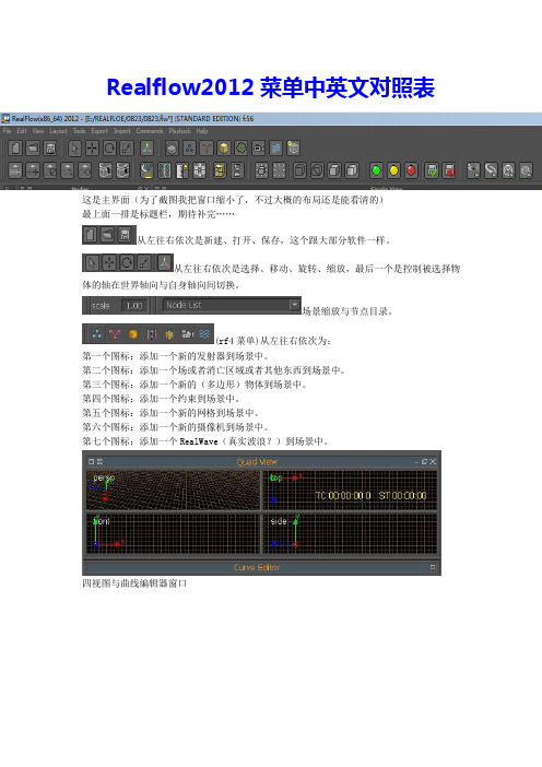
Realflow2012菜单中英文对照表这是主界面(为了截图我把窗口缩小了,不过大概的布局还是能看清的)最上面一排是标题栏,期待补完……从左往右依次是新建、打开、保存,这个跟大部分软件一样。
从左往右依次是选择、移动、旋转、缩放,最后一个是控制被选择物体的轴在世界轴向与自身轴向间切换。
场景缩放与节点目录。
(rf4菜单)从左往右依次为:第一个图标:添加一个新的发射器到场景中。
第二个图标:添加一个场或者消亡区域或者其他东西到场景中。
第三个图标:添加一个新的(多边形)物体到场景中。
第四个图标:添加一个约束到场景中。
第五个图标:添加一个新的网格到场景中。
第六个图标:添加一个新的摄像机到场景中。
第七个图标:添加一个RealWave(真实波浪?)到场景中。
四视图与曲线编辑器窗口Nodes(上左):节点Exclusive Links(上中):独有连接、单独连接Global Links(上右):总体连接、全局连接Node Params(下左):节点参数Messages(下右):信息时间控制区期待补完……动画控制区期待补完……发射器(emitter)篇Circle:圆形发射器Square:矩形发射器Sphere:球形发射器Linear:线形发射器Triangle:三角形发射器Spline:曲线发射器Cylinder:圆柱形发射器Bitmap:位图发射器Object emitter:物体发射器Fill Object:填充物体RW_Splash:RW飞溅RW_Particles:RW粒子Fibers:纤维发射器Binary Loader:NBinary Loader:节点参数菜单:公共参数:Node:节点Simulation:模拟Position:方位 Inactive:无效、不活动Rotation:旋转 Active:有效、活动Scale:缩放 Cache:缓存Pivot:枢轴、中心点Parent to:连接到父物体Color:颜色Xform particles:变换粒子 Yes/No:是/否(下文同)Initial state:初始状态Use initial state:使用初始状态Make initial state:生成初始状态Particles:粒子Type:类型 Gas:气体Resolution:分辨率Density:密度Int pressure:内压力Ext pressure:外压力Viscosity:粘性Temperature:温度Ext temperature:表面温度Heat capacity:热能Heat conductivity:热传导Compute vorticity:计算涡流Max particles:最大粒子数量Particles:粒子Type:类型 Liquid:液体Resolution:分辨率Density:密度Int pressure:内压力Ext pressure:外压力Viscosity:粘性Surface tension:表面张力Interpolation:插补 None:无Compute vorticity:计算涡流 Local:局部Max particles:最大粒子数量 Global:总体、全局Particles:粒子Type:类型 Dumb:哑、无声Resolution:分辨率Density:密度Max particles:最大粒子数量Particles:粒子Type:类型 Elastics:弹性体、橡皮带Resolution:分辨率Density:密度Spring:弹力Damping:阻尼Elastic limit:Break limit:Max particles:最大粒子数量Particles:粒子Type:类型 Custom:自定义Resolution:分辨率Density:密度Int pressure:内压力Ext pressure:外压力Viscosity:粘性Temperature:温度Max particles:最大粒子数量Edit:编辑Statistics:统计Existent particles:存在粒子数量Emitted particles:发射粒子数量Particle mass:粒子质量V min:V最小值V max:V最大值Display:显示Visible:可见性Point size:粒子点大小Show arrows:显示箭头Arrow length:箭头长度Property:属性Automatic range:自动距离Min range:最小距离 Velocity:速度Min range color:最小距离颜色 Velocity X:速度的X方向Max range:最大距离 Velocity Y:速度的Y方向Max range color:最大距离颜色 Velocity Z:速度的Z方向Pressure:压力Density:密度Vorticity:涡流Temperature:温度Constant:固定独立参数:Circle:圆形发射器Volume:体积Speed:速度V random:V随机H random:H随机Ring ratio:环形比例Side emission:边线发射Square:矩形发射器Volume:体积Speed:速度V random:V随机H random:H随机Side emission:边线发射Sphere:圆形发射器Speed:速度Randomness:随机Fill sphere:填充球体发射器Linear:线形发射器Height:高度Length:长度Speed:速度V random:V随机H random:H随机Triangle:三角形发射器Volume:体积Speed:速度V random:V随机H random:H随机Side emission:边线发射Bitmap:位图发射器Emission mask:发射面具File list:文件目录 Single:单帧Number of files:文件数目 Sequence-end:序列末端Affect:影响 Sequence-keep:保持序列Val min:最小值 Sequence-loop:循环序列Val max:最大值Volume:体积Speed:速度V random:V随机 None:无H random:H随机 Viscosity:可见Spline:曲线发射器Affect:影响Creation:创建Speed:速度 Force:力Randomness:随机 Velocity:速度Kill leaving:消除残留Edit:编辑Insert CP:插入CPDelete CP:删除CP@ CP index:CP索引 Axis:轴@ CP axial:CP轴向 Tube:圆管@ CP radial:CP放射 Edge:边@ CP vortex:CP涡流@ CP radius:CP半径@ CP rotation:CP旋转@ CP link:CP连接Cylinder:圆柱形发射器Speed:速度V random:V随机H random:H随机Object emitter:物体发射器Object:物体Parent velocity per:每父物体速度Distance threshold:距离起点Jittering:抖动Speed:速度Randomness:随机Smooth normals:平滑法线Use texture:使用纹理Select Faces:选择面Select Vertex:选择点Clear selection:清除选择Fill Object:填充物体Object:物体Fill Volume:填充体积Fill X radio:填充X半径Fill Y radio:填充Y半径Fill Z radio:填充Z半径Remove # layers:移除层Jittering:抖动@ seed:种子值Particle layer:粒子层RW_Splash:RW飞溅Object:物体Waterline mult:吃水线倍率@ H strength:H强度@ V strength:V强度@ Side emission:边线发射@ Normal speed:法线速度Underwater mult:水下倍率@ Depth threshold:深度起点Speed mult:速度倍率Parent Obj Speed:父物体速度Speed threshold:速度起点Speed variation:速度变化Drying speed:干燥速度RW_Particles:RW粒子Speed:速度Speed variation:速度变化Height for emission:发射高度Speed for emission:发射速度Fibers:纤维发射器Object:物体Length:长度Length variation:长度变化Threshold:起点Stiffness:硬度Fiber damping:纤维阻尼Interpolate:窜改Select Vertex:选择点Clear selection:清除选择Create:创建Mesh tube:网格圆管@ Mesh width:网格宽度@ Mesh width end:网格末端宽度@ Mesh section:网格切片Binary Loader:二进制装入程序BIN sequence:本系列Mode:形式方法Reverse:反向的Number of files:文件数Frame Offset:帧偏移Release particles:释放粒子Load particles:负荷粒子Reset xform:变换重置Subdivisions:分支机构@ Output sequence:输出序列NBinary Loader:****装载机BIN sequences:本序列Load Bin Seq:负载箱序列Remove Bin Seq:删除本条Mode:模式Reverse:反向的Number of files:文件数Frame offset:帧偏移Reset xform:变换重置力场与消亡区域(daemon)篇k Volume:体积消亡k Age:年龄消亡k Speed:速度消亡k Isolated:隔离消亡k Collision:碰撞消亡k Sphere:球形消亡Gravity:重力场Attractor:吸引器DSpline:曲线力场Wind:风力场Vortex:漩涡场Layered Vortex:分层漩涡Limbo:不稳定状态Tractor:牵引器Coriolis:向心力场Ellipsoid force:椭球力场Drag force:拖动力场Surface tension:表面张力Noise field:噪波场Heater:加热器Texture Gizmo:Magic:魔术Object field:物体场Color plane:色彩平面Scripted:脚本节点参数菜单:公共参数:(请参考发射器篇公共参数节点一栏,一模一样,在此省略)独立参数:k Volume:体积消亡Fit to object:适配到物体Fit to scene:适配到场景Inverse:翻转k Age:年龄消亡Iife:生命值Variation:变化Split:分裂@ # child:子物体数量k speed:速度消亡Min speed:最小速度Max speed:最大速度Limit & keep:限制与保持Split:分裂@ # child:子物体数量Bounded:边界Boundary:边界范围k Isolated:隔离消亡Isolated time:隔离时间k Collision:碰撞消亡All objects:所有物体Select objects:选择物体Split:分裂@ # child:子物体数量k Sphere:球形消亡Fit to object:适配到物体Fit to scene:适配到场景Radius:半径Inverse:翻转Gravity:重力场Affect:影响Strength:强度 Force:力Bounded:边界 Velocity:速度Underwater:水下No:无Box:立方体Plane:平面Push:扩展Attractor:吸引器Affect:影响Internal force:内力 Force:力Internal radius:内半径 Velocity:速度External force:外力External radius:外半径Attenuated:衰减Attractor type:吸引类型Planet radius:圆球半径 Spherical:球形Axial strength:轴向强度 Axial:轴向Bounded:边界 Planetary:不定向Dspline:曲线力场Affect:影响Vortex strength:涡流强度Axial strength:轴向强度 force:力Radial strength:辐射强度 velocity:速度Bounded:边界Edit:编辑Insert CP:插入CPDelete CP:删除CP@ CP index:CP索引@ CP axial:CP轴向@ CP radial:CP放射@ CP vortex:CP涡流@ CP radius:CP半径@ CP link:CP连接Wind:风力场Affect:影响Strength:强度Noise strength:噪波强度Noise scale:噪波缩放 Force:力Bounded:边界 Velocity:速度@ radius 1:半径1@ radius 2:半径2@ height:高度Vortex:漩涡场Affect:影响Rot strength:旋转强度 Force:力Central strength:中心强度 Velocity:速度Attenuation:衰减Bounded:边界Boundary:边界范围Vortex type:涡流类型Radius:半径 Linear:线性Bound Sup: Square:平方Bound Inf: Cubic:立方Classic:经典Complex:复合Layered Vortex:分层漩涡Affect:影响Num layers:分层数量Offset:偏移 Force:力Current Layer:当前层 Velocity:速度@ Vortex type:涡流类型@ Strength:强度@ Radius:半径@ Width:宽度 Classic:经典@ Bounded:边界 Complex:复合@ Boundary:边界范围Limbo:不稳定状态Affect:影响Width:宽度Strength 1:强度1 Force:力Attenuate 1:衰减1 Velocity:速度Strength 2:强度2Attenuate 2:衰减2Tractor:牵引器Affect:影响F1 Force:力F2 Velocity:速度F3F4Coriolis:向心力场Affect:影响 Force:力Strength:强度 Velocity:速度Ellipsoid force:椭球力场Min velocity:最小速度Min gain:最小增量Max velocity:最大速度Max gain:最大增量Clamp:钳紧Drag force:拖动力场Drag strength:拖动强度Shield effect:盾效果 No:无@ shield inverse:盾翻转 Square:正方形Force limit:力量限制 Sphere:圆形Bounded type:边界类型Attenuation:衰减 No:无Affect vertex:影响点 linear:线性Square:平方Cubic:立方Surface tension:表面张力Strength:强度balanced:平衡Noise field:噪波场Affect:影响Strength:强度 Force:力Scale Factor:缩放系数 Velocity:速度Bounded:边界Radius:半径多边形物体(object)篇Null:点Sphere:球体Hemisphere:半球体Cube:立方体Cylinder:圆柱体Vase:花瓶、杯子、碗Cone:圆锥体Plane:平面Torus:圆环体Rocket:火箭Capsule:胶囊Import:导入节点参数菜单:公共参数:Node:节点Simulation:模拟 Inactive:无效、不活动Dynamics:动力学 Active:有效、活动Position:方位 Cache:缓存Rotation:旋转Scale:缩放Pivot:枢轴、中心点Parent to:连接到父物体Color:颜色 No:无SD<->Curve:SD文件与曲线互转 Rigid body:刚体Initial state:初始状态Soft body:柔体Use initial state:使用初始状态Make initial state:生成初始状态Texture:纹理Load Texture:读取纹理WetDry texture:@ resolution:分辨率@ filter loops #:过滤循环@ filter strength:过滤强度@ pixel strength:像素浓度@ ageing:时效Display:显示Visible:可见性Show normals:显示法线Show particles:显示粒子Normal size:法线大小 Face:面Normal type:法线类型 Vertex:点Reverse normals:翻转法线 VtxFace:Show texture:显示纹理独立参数:无约束(constraint)篇Ball_socket:球形槽Hinge:铰链Slider:滑动Fixed:固定Rope:捆绑Path_follow:跟随路径Car_wheel:滚动Limb:网格(mesh)篇节点参数菜单:Mesh:网格Build:创建 Metaballs:变形球Type:类型 Mpolygons:Clone obj:复制物体 Clone obj:复制物体Polygon size:多边形大小@ Num Faces:面数LOD resolution:细节级别分辨率@ Camera:摄像机 No:无@ Min distance:最小距离 Camera:摄像机@ Min Polygon size:最小多边形大小@ Max distance:最大距离@ Max Polygon size:最大多边形大小Texture:纹理UVW Mapping:UVW贴图Load texture:读取纹理Tiling:贴砖Appy map now:现在应用贴图Speed info:速度信息 None:无Filters:过滤 UV particle:UV粒子Filter method:过滤方法 UV sprite:UV精灵Relaxation:松弛 Speed:速度Tension:张力、拉紧 Pressure:压力Steps:步数 Temperature:温度Clipping:限制、剪裁Clipping box:限制立方体Clipping objects:限制物体InOut clipping:内外限制Camera clipping:摄像机限制Camera:摄像机 Inside:内部Realwave clipping:Realwave限制 Outside:外部Optimize:优化Optimize:优化Camera:摄像机Merge Iterations:融合迭代次数@ Ite threshold:迭代阈值 No:无Face subdivision:表面细分 Curvature:曲率@ Sub threshold:细分阈值 Camera:摄像机Display:显示Color:颜色Transparency:透明度Back face culling:背面消隐与网格关联的粒子发射器(比如:)节点参数菜单:Field:区域Blend factor:融合系数Radius:半径Subtractive field:负(相反)区域Noise:噪波Fractal noise:分型噪波@ Amplitude:振幅@ Frequency:频率@ Octaves:倍频程Deformation:变形Speed stretching:拉伸速度Min str scale:最小拉伸缩放Max str scale:最大拉伸缩放Speed flattening:压扁速度Min flat scale:最小压扁速度Max flat scale:最大压扁速度Min speed:最小速度Max speed:最大速度摄像机(camera)篇Realwave篇节点参数菜单:显示网格流体菜单范围,领域发射体泡沫飞溅湿泡沫泼溅湿的下雨的泡沫船的吃水线雾水汽每段的飞溅每段的泡沫每段的雾菜单栏第二排(rf2012)1.transformations:变换2.position :位置3.scale :刻度尺度4.shear:剪切5.rotation :旋转6. 最近的侧面7.最近的侧面(拓展)8. 粒子工具9. 粒子的选择10. 测量工具11 创建数组12 破裂13. 回复时间模拟14 设置选定可见15 设置选定的隐藏16. 设置选定的包围盒17. 设置选定的线框18. 设置选定的闪光阴影19. 设置选定的平滑阴影20. 设置选定的活动21. 设置选定的缓存22. 设置选定的无效23.设置选定的出口数据24. 禁用数据输出选择25. 改变分辨率26.计算vorticiy27.正常年龄28. 建立网格右下角控制栏1.建立网格2. 硬化方法3. 可视化细节层次4. 发送给招聘经理5. 去上关键帧6. 去下个关键帧7. 设置一个关键帧中的当前位置图层1.可见物视程2. 模仿模拟3. 层4. 可见的已有的5. 显示模式6.增加新的层与选定的节点7.流体动力学对象的动态显示网格菜单粒子网格粒子网格(标准)网格网格显示的菜单单一的多样的。
Incomplete equilibrium in long-range interacting systems
a r X iv :c o n d -m a t /0603659v 2[c o n d -m a t.st a t-m e c h ]13S e p 2006Incomplete equilibrium in long-range interacting systemsFulvio Baldovin and Enzo Orlandini ∗Dipartimento di Fisica and Sezione INFN,Universit`a di Padova,Via Marzolo 8,I-35131Padova,Italy(Dated:February 6,2008)We use a Hamiltonian dynamics to discuss the statistical mechanics of long-lasting quasi-stationary states particularly relevant for long-range interacting systems.Despite the presence of an anomalous single-particle velocity distribution,we find that the Central Limit Theorem implies the Boltzmann expression in Gibbs’Γ-space.We identify the nonequilibrium sub-manifold of Γ-space characterizing the anomalous behavior and show that by restricting the Boltzmann-Gibbs approach to this sub-manifold we obtain the statistical mechanics of the quasi-stationary states.PACS numbers:05.20.-y,05.70.Ln,05.10.-aIn comparison with its equilibrium counterpart,nonequilibrium statistical mechanics does not rely on uni-versal notions,like the ensembles ones,through whichone can handle large classes of physical systems [1].In-complete (or partial)equilibrium states [2,3]are in thisrespect a remarkable exception,since in these cases con-cepts of equilibrium statistical mechanics can be usedto describe nonequilibrium situations.Incomplete equi-librium states arise when different parts of the systemthemselves reach a state of equilibrium long before theyequilibrate with each other [2].The classical understand-ing on how a system approaches equilibrium is based onthe short time-scale collisions mechanism which links anyinitial condition to the statistical equilibrium.For long-range interacting systems,this picture is not valid any-more since the time-scale for microscopic collisions di-verges with the range of the interactions.This impliesthat the Boltzmann equation must be substituted withother approximations such as the Vlasov or the Balescu-Lenard equations [4],where the interparticle correlationsare negligible or almost negligible and a nonequilibriuminitial configuration could stay frozen or almost frozenfor a very long time.This applies,e.g.,to gravitationalsystems,Bose-Einstein condensates and plasma physics[5].Due to the physical relevance of long-range interact-ing systems and to the privileged position of incompleteequilibrium states in nonequilibrium statistical mechan-ics,it is important to investigate whether the notion ofincomplete equilibrium plays an important role in under-standing the nonequilibrium properties of these systems.Recently we showed [6]that nonequilibrium statesin which the value of macroscopic quantities remainsstationary or quasi-stationary for reasonably long time(quasi-stationary states –QSSs)are important,e.g.,forexperiments,since they appear even when the long-rangesystem exchanges energy with a thermal bath (TB).Us-ing the same paradigmatic long-range interacting systemof Ref.[6],the Hamiltonian Mean Field (HMF)model[7],here we discuss the Gibbs’Γ-space statistical mechan-2+1Hamiltonian in Eq.(1)can be considered as an interest-ing“paradigm”for long-range interacting systems[12]. The TB introduced in[6]is characterized by N≫M equivalent spinsfirst-neighbors coupled along a chainH TB=N i=M+1l2ifor M=10),distinguishing the canonical QSSs from the microcanonical ones.We now address the main result of the paper,which is central to the discussion of the appropriate statistical mechanics approach for quasi-stationary nonequilibrium states in long-range systems and to the debate in[8,9,10,11].According to BG,the equilibrium PDF of the energyE for a system in contact with a TB at temperature T is p BG(E)=ω(E)e−E/T/Z,where Z is the partition function.Since the Hamiltonian simulations consent an empirical estimation of this PDF,it is possible to verify p BG(E)on dynamical basis[16].From the analytically known solution of the HMF model[7,12]one obtains the BG equilibrium caloric curve of the system T(E)(full line in Fig.2a).The integration of the thermodynamic relation∂lnω(E)/∂E=1/T(E),ln[ω(E)]−ln[ω(E0)]= E E0dE′1son with the dynamical simulations results.Specifically, we show below that T corresponds to twice the specific kinetic energy of the HMF.The HMF caloric curve atfixed m HMF= m HMF is given,for all m HMF ∈[0,1],by the straight lineE HMFT HMF, m (E HMF)=2。
Fluent中用户自定义函数应用举例
第10章应用举例本章包含了FLUENT中UDFs的应用例子。
10.1 边界条件10.2源项10.3物理属性10.4反应速率(Reacting Rates)10.5 用户定义标量(User_Defined Scalars)10.1边界条件这部分包含了边界条件UDFs的两个应用。
两个在FLUENT中都是作为解释式UDFs被执行的。
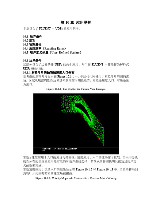
10.1.1涡轮叶片的抛物线速度入口分布要考虑的涡轮叶片显示在Figure 10.1.1中。
非结构化网格用于模拟叶片周围的流场。
区域从底部周期性边界延伸到顶部周期性边界,左边是速度入口,右边是压力出口。
Figure 10.1.1: The Grid for the Turbine Vane Example常数x速度应用于入口的流场与抛物线x速度应用于入口的流场作了比较。
当采用分段线性分布的型线的应用是有效的对边界型线选择,多项式的详细说明只能通过用户定义函数来完成。
常数速度应用于流场入口的结果显示在Figure 10.1.2和Figure 10.1.3中。
当流动移动到涡轮叶片周围时初始常速度场被扭曲。
Figure 10.1.2: Velocity Magnitude Contours for a Constant Inlet x VelocityFigure 10.1.3: Velocity Vectors for a Constant Inlet x Velocity现在入口x速度将用以下型线描述:这里变量y在人口中心是0.0,在顶部和底部其值分别延伸到0745。
这样x速度在.0入口中心为20m/sec,在边缘为0。
UDF用于传入入口上的这个抛物线分布。
C源代码(vprofile.c)显示如下。
函数使用了Section 5.3中描述的Fluent提供的求解器函数。
/***********************************************************************//* vprofile.c *//* UDF for specifying steady-state velocity profile boundary condition *//***********************************************************************/#include "udf.h"DEFINE_PROFILE(inlet_x_velocity, thread, position){real x[ND_ND]; /* this will hold the position vector */real y;face_t f;begin_f_loop(f, thread){F_CENTROID(x,f,thread);y = x[1];F_PROFILE(f, thread, position) = 20. - y*y/(.0745*.0745)*20.;}end_f_loop(f, thread)}函数,被命名为inlet_x_velocity,使用了DEFINE_PROFILE定义并且有两个自变量:thread 和position。
Can Short-Range Interactions Mediate a Bose Metal Phase in 2D
a r X i v :c o n d -m a t /0109269v 1 14 S e p 2001Can Short-Range Interactions Mediate a Bose Metal Phase in 2D?Philip Phillips 1and Denis Dalidovich 21Loomis Laboratory of PhysicsUniversity of Illinois at Urbana-Champaign 1100W.Green St.,Urbana,IL,61801-30802National High Magnetic Field LaboratoryFlorida State University,Talahasse,Florida,31301We show here based on a 1-loop scaling analysis that short-range interactions are strongly irrelevant perturbations near the insulator-superconductor (IST)quantum critical point.The lack of any proof that short-range interactions mediate physics which is present only in strong coupling leads us to conclude that short-range interactions are strictly irrelevant near the IST quantum critical point.Hence,we argue that no new physics,such as the formation of a uniform Bose metal phase can arise from an interplay between on-site and nearest-neighbour interactions.The standard model used to study [1–13]the insulator-superconductor transition in thin films is the commensu-rate Bose-Hubbard model or equivalently the charging model for an array of Josephson junctions.The Hamil-tonian for this modelˆH=12dτk˙φ(k )˙φ(−k)no restriction on the range of V ij.To simplify this action, wefirst decouple the charging term by introducing[4]an auxilliary real gaugefield,A0(k),through the identity exp −1V(k)˙φ(−k) = D A0exp −1e−2V(k)−1−12 d d xdτ |(∂τ−ieA0)ψ|2+|∇ψ|2+r|ψ|2+u 2 k,ωA0(k,ω)A0(−k,−ω)2 k,ωkσA0(k,ω)A0(−k,−ω),(7) which is the Fisher and Grinstein[4]result.What about short-range interactions?We simplify to the case considered by Das and Doniach[21]and truncate V(k)at the nearest-neighbour level:V(k)=V0+2V1(cos k x+cos k y).(8) It is crucial in our derivation that V0=0.As has been considered previously,when V0=0but V1=0,the na-ture of the T=0transition changes fundamentally when compared with the V0=0case.In the former case,that is,V0=0but V1=0,the T=0transition is of the Berezinskii-Kosterlitz-Thouless kind[23].In the long wavelength limit,V(k)=V0+2V1−V1k2,which is con-venient to write in the form,e2−V1k2where we have fixed the free parameter,e2=V0+2V1.Consequently, the pure gauge part of the action simplifies toS1=−e2k2.(9) Uponrescaling the gaugefield,A0(k,ω)→i e2A0(k,ω),we arrive at the working form for the action,S=12|ψ|4 +1k2A0(k,ω)(10)where the constant g= V1. Clearly,when V1=0,g=0and the rescaledfields, A0(k,ω),vanish leading to the standard on-site charging model.Hence,the relevance of short range interactions can be deduced entirely from the scaling properties of the coupling constant g.Performing the standard tree-level rescaling with the rescaling parameter b>1,wefind that the momentum and frequency scale as q′=qb andω′=ωb z,with z the dynamical exponent.At the tree level,z=1and the anomalous dimension exponent vanishes,η=0.Hence, theψand A0fields scale asA0=bµA′0,µ=d+z−22.(11) Combining these scaling relations with the rescaling of the momentum and the frequency arising from the inte-grations in the action,we arrive at our key resultg′=gbµ+λWe evaluate these diagrams using the standard frequency-momentum shell RG approach in which we in-tegrate out thefields A0(ω,k)andψ(ω,k)for momenta and frequencies satisfying the constraintΛb <k<Λwith the upper momentum and frequencycutoffsΛω=Λk=Λ=1.Setting b=eℓ,we obtain dgℓ2 gℓ−2Aℓgℓuℓ−Bℓg3ℓ(13) as the differential form for the scaling equation for g.The coefficients,Aℓand Bℓare given byAℓ=2K d(q2+1+rℓ)2 + 10dω(2π)d+1 10dqq d+11+2q2+2rℓ(1+ω2+rℓ)2 ,(15) where K d is the area of a d-dimensional unit sphere. These coefficients are positive and depend on the scal-ing lengthℓthrough the parameter rℓ.Hence,fromthestructureofthescaling equation,for gℓ,Eq.(13),wefindthat the g=0fixed point is stable through one-loop or-der.That is,there is no signature in weak coupling thatfinite g can drive a new critical point.This conclusionis consistent with the standard view that as long as thebroken symmetry state is rotationally and translation-ally invariant,the critical point is of the Wilson-Fishertype where it is well known that short-range interactionscannot lead to a new critical point.Because g∝√[1]S.Doniach,Phys.Rev.B24,5063,(1981).[2]M.P.A.Fisher,Phys.Rev.B36,1917(1987);[3]X.G.Wen and A.Zee,Int.J.Mod.Phys.B4,437(1990).[4]M.P.A.Fisher and G.Grinstein,Phys.Rev.Lett.60,208,(1988).[5]W.Zwerger,J.Low Temp.Phys.72,291(1988);ibid,Physica B152,236(1988).[6]S.Chakravarty,S.Kivelson,G.T.Zimanyi,and B.I.Halperin,Phys.Rev.B37,3283(1988).[7]A.Kampf and G.Sch¨o n,Phys.Rev.B36,3651(1987).[8]V.Ambegoakar,U.Eckern,and G.Sch¨o n,Phys.Rev.Lett.48,1745(1982).[9]K.Wagenblast,A.van Otterlo,G.Sch¨o n,and G.Zi-manyi,Phys.Rev.Lett.79,2730(1997).[10]A.van Otterlo,K.-H Wagenblast,R.Fazio,and G.Sch¨o n,Phys.Rev.B48,3316(1993).[11]M.C.Cha,M.P.A.Fisher,S.M.Girvin,M.Wallin,and A.P.Young,Phys.Rev.B44,6883(1991).[12]E.Frey and L.Balents,Phys.Rev.B55,1050(1997).[13]F.Hebert,G.G.Batrouni,R.T.Scalettar,G.Schmid,M.Troyer,and A.Dorneich,cond-mat/0105450.[14]N.Mason and A.Kapitulnik,Phys.Rev.Lett.82,5341(1999);ibid,cond-mat/0006138.[15]D.Ephron, A.Yazdani, A.Kapitulnik,and M.R.Beasley,Phys.Rev.Lett.76,1529(1996).[16]H.M.Jaeger,D.B.Haviland,B.G.Orr,and A.M.Goldman,Phys.Rev.B40,182(1989).[17]H.S.J.van der Zant,et.al.Phys.Rev.B54,10081,(1996).[18]D.Dalidovich and P.Phillips,Phys.Rev.B64,52507-1(2001).[19]E.Shimshoni,A.Auerbach,and A.Kapitulnik,Phys.Rev.Lett.80,3352(1998).[20]A.Kapitulnik,N.Mason,S. A.Kivelson,and S.Chakravarty,cond-mat/0009201.[21]D.Das and S.Doniach,Phys.Rev.B601261(1999).[22]See Eq.4.11in J.Cardy,Scaling and Renormalization inStatistical Physics,(Cambridge University Press,Cam-bridge,1996)p.71.[23]R.Fazio and G.Sch¨o n,Phys.Rev.43,5307(1991).[24]Jinwu Ye,Phys.Rev.B58,9450(1998).3。
Chapter 21. Modeling Solidification and Melting
This chapter describes how you can model solidification and melting in rmation is organized into the following sections:•Section21.1:Overview and Limitations of the Solidification/MeltingModel•Section21.2:Theory for the Solidification/Melting Model•Section21.3:Using the Solidification/Melting Model21.1Overview and Limitations of theSolidification/Melting Model21.1.1OverviewFLUENT can be used to solvefluidflow problems involving solidification and/or melting taking place at one temperature(e.g.,in pure metals)or over a range of temperatures(e.g.,in binary alloys).Instead of tracking the liquid-solid front explicitly,FLUENT uses an enthalpy-porosity for-mulation.The liquid-solid mushy zone is treated as a porous zone with porosity equal to the liquid fraction,and appropriate momentum sink terms are added to the momentum equations to account for the pressure drop caused by the presence of solid material.Sinks are also added to the turbulence equations to account for reduced porosity in the solid regions.FLUENT provides the following capabilities for modeling solidification and melting:•Calculation of liquid-solid solidification/melting in pure metals aswell as in binary alloysc Fluent Inc.November28,200121-1Modeling Solidification and Melting21.2Theory for the Solidification/Melting ModelModeling Solidification and Meltingif T solidus<T<T liquidus(21.2-3)T liquidus−T solidusEquation21.2-3is referred to as the lever rule.Other relationships be-tween the liquid fraction and temperature(and species concentrations) are possible,but are not considered here.The latent heat content can now be written in terms of the latent heat of the material,L:∆H=βL(21.2-4) The latent heat content can vary between zero(for a solid)and L(for a liquid).For solidification/melting problems,the energy equation is written as∂21.2Theory for the Solidification/Melting ModelA mush( v− v p)(21.2-6)(β3+ )whereβis the liquid volume fraction, is a small number(0.001)to prevent division by zero,A mush is the mushy zone constant,and v p is the solid velocity due to the pulling of solidified material out of the domain (also referred to as the pull velocity).The mushy zone constant measures the amplitude of the damping;the higher this value,the steeper the transition of the velocity of the mate-rial to zero as it solidifies.Very large values may cause the solution to oscillate.The pull velocity is included to account for the movement of the solidified material as it is continuously withdrawn from the domain in continuous casting processes.The presence of this term in Equation21.2-6allows newly solidified material to move at the pull velocity.If solidified mate-rial is not being pulled from the domain, v p=0.More details about the pull velocity are provided in Section21.2.4.21.2.3Turbulence EquationsSinks are added to all of the turbulence equations in the mushy and solidified zones to account for the presence of solid matter.The sink term is very similar to the momentum sink term(Equation21.2-6):(1−β)2S=Modeling Solidification andMelting mushy zone solidified shellpFigure 21.2.1:“Pulling”a Solid in Continuous CastingAs mentioned in Section 21.2.2,the enthalpy-porosity approach treats the solid-liquid mushy zone as a porous medium with porosity equal to the liquid fraction.A suitable sink term is added in the momentum equation to account for the pressure drop due to the porous structure of the mushy zone.For continuous casting applications,the relative velocity between the molten liquid and the solid is used in the momentum sink term (Equation 21.2-6)rather than the absolute velocity of the liquid.The exact computation of the pull velocity for the solid material is de-pendent on the Young’s modulus and Poisson’s ratio of the solid and the forces acting on it.FLUENT uses a Laplacian equation to approxi-mate the pull velocities in the solid region based on the velocities at the boundaries of the solidified region:21-6cFluent Inc.November 28,200121.2Theory for the Solidification/Melting Model(21.2-9)(l/k+R c(1−β))where T,T w,and l are defined in Figure21.2.2,k is the thermal conduc-tivity of thefluid,βis the liquid volume fraction,and R c is the contact resistance,which has the same units as the inverse of the heat transfer coefficient.c Fluent Inc.November28,200121-7Modeling Solidification and Melting21.3Using the Solidification/Melting ModelModeling Solidification and Melting21.3Using the Solidification/Melting ModelModeling Solidification and Melting21.3Using the Solidification/Melting ModelModeling Solidification and Melting。
The B-Supergiant Components of the Double-Lined Binary HD1383
a rXiv:as tr o-ph/64247v111Apr26The B-Supergiant Components of the Double-Lined Binary HD 1383T.S.Boyajian,D.R.Gies 1,M.E.Helsel 2,A.B.Kaye 1,M.V.McSwain 1,3,4,R.L.Riddle 1,5,D.W.Wingert 1Center for High Angular Resolution Astronomy and Department of Physics and Astronomy,Georgia State University,P.O.Box 4106,Atlanta,GA 30302-4106;tabetha@,gies@,marian.helsel@,anthony.kaye@,mcswain@,riddle@,wingert@ ABSTRACT We present new results from a study of high quality,red spectra of the massive binary star system HD 1383(B0.5Ib +B0.5Ib).We determined radial veloci-ties and revised orbital elements (P =20.28184±0.0002d)and made Doppler tomographic reconstructions of the component spectra.A comparison of these with model spectra from non-LTE,line blanketed atmospheres indicates that both stars have almost identical masses (M 2/M 1=1.020±0.014),temperatures (T eff=28000±1000K),gravities (log g =3.25±0.25),and projected rotational velocities (V sin i 30km s −1).We investigate a number of constraints on the radii and masses of the stars based upon the absence of eclipses,surface grav-ity,stellar wind terminal velocity,and probable location in the Perseus spiral arm of the Galaxy,and these indicate a range in probable radius and mass ofR/R ⊙=14−20and M/M ⊙=16−35,respectively.These values are consistentwith model evolutionary masses for single stars of this temperature and gravity.Both stars are much smaller than their respective Roche radii,so the systemis probably in a pre-contact stage of evolution.Afit of the system’s spectralenergy distribution yields a reddening of E(B−V)=0.55±0.05and a ratioof total-to-selective extinction of R=2.97±0.15.Wefind no evidence of Hαemission from colliding stellar winds,which is probably the consequence of thelow gas densities in the colliding winds zone.Subject headings:binaries:spectroscopic—stars:early-type—stars:evolution—stars:individual(HD1383)—supergiants—stars:winds,outflows1.IntroductionThe evolutionary paths of massive binaries depend critically on processes related to mass transfer and mass loss at the time when the initially more massive star begins tofill its Roche volume(Langer et al.2004;Petrovic,Langer,&van der Hucht2005).On the one hand,mass from the donor star may end up entirely in a rejuvenated mass gainer,but on the other hand a high mass transfer rate may cause the gainer to swell and bring the system into a common envelope phase,in which most of the donor’s mass is lost from the system entirely. Evidence of both outcomes is found among post-Roche lobe overflow systems(Langer et al. 2004;Petrovic et al.2005).We can better constrain the problem of the probable results of the interaction by studying binaries in an advanced evolutionary state just prior to Roche-filling.Those binaries of nearly identical masses are particularly interesting because we can usually observe the spectra of both components.Close pairs of nearly identical,evolved massive stars are quite rare.The HD1383system is the only such system found in Ninth Catalogue of Spectroscopic Binary Orbits(Pourbaix et al.2004)(with identical components of types B0.5Ib+B0.5Ib;Hill&Fisher1986).Another similar massive stellar system,HD152248,was previously classified as a O7I+O7I(Penny, Gies,&Bagnuolo1999),although a more thorough analysis by Sana et al.(2001)revised the classifications to O7.5III+O7III,deviating from the exact match of types found in HD1383.The HD152248system is eclipsing and the mass determinations made by Penny et al.(1999)and Sana et al.(2001)indicate that both stars are undermassive(by factors of 2and1.4,respectively,in the two studies)relative to the predicted evolutionary masses for single stars.Here we focus our attention on HD1383(BD+60◦25,HIP1466).The system was identified as a double-lined binary early on(Sanford&Merrill1938;Slettebak1956), but thefirst orbital elements were determined later by Hill&Fisher(1986)who found that the system consists of two nearly identical stars with an orbital period of20.3d.Morgan,Code,&Whitford(1955)originally adopted the system as a spectral standard for the B1II type,but Hill&Fisher(1986)revised the types slightly based upon detailed measurements of line equivalent widths of both components.The system is located in the sky in the vicinity of the Cas OB4association(Humphreys1978),which is located in the Perseus arm of the Galaxy.The star has played an important role in studies of the interstellar medium in this direction(see Cartledge et al.2004).Various distances have been estimated based upon the assumption that HD1383is a single,B1II star.Wakker et al.(1998)found a distance of 1.7kpc,which agrees well with Humphreys(1978)value of1.68kpc.Humphreys(1978) noted that HD1383might not be a member of the Cas OB4association,because the latter has a greater distance of2.88kpc.However,the fact that HD1383is a binary consisting of two stars with approximately equal brightness implies that it farther away from us than these previous estimates indicate and that it is closer to Cas OB4(Hill&Fisher1986offer a distance3.0kpc for HD1383).Here we present a study of a set of red spectra of HD1383that we obtained(§2)to re-analyze the orbital elements(§3)and to search for evidence of Hαemission related to colliding winds(Thaller1997;Sana et al.2001).We discuss the physical parameters of the stars from an analysis of their individual spectra obtained from a Doppler tomography reconstruction(§4).We then present a number of constraints on the radii and masses of the stars(§5)that lead us to conclude that both stars have radii smaller than their Roche radii and luminosities that are too small to power strong winds(explaining the lack of Hαemission from colliding winds).2.Observations and Radial VelocitiesThe optical spectra of HD1383were obtained with the Kitt Peak National Observatory 0.9m coud´e feed telescope during four observing runs between1999August and1999De-cember.Most of these spectra were obtained with the short collimator and grating RC181 (316grooves mm−1with a blaze wavelength of7500˚A;made infirst order with a GG495filter to block higher orders),which yielded an average resolving power of R=λ/δλ=4000 (see Gies et al.2002a for details of each observing run).The last four spectra were made with grating B(632grooves mm−1with a blaze wavelength of6000˚A in second order)and these have a much higher resolving power,R=λ/δλ=21300.Exposure times varied from 20to30minutes.These spectra all cover a common spectral range between6456˚A and 6728˚A,and they generally have a S/N≈340pixel−1in the continuum.The spectra wereextracted and calibrated using standard routines in IRAF6,and then each continuum rec-tified spectrum was transformed onto a uniform heliocentric wavelength grid for analysis. Atmospheric telluric lines were removed by division of modified versions of spectra of the rapidly rotating A-starζAql that we also observed(Gies et al.2002a).We measured radial velocities for HD1383using a templatefitting method(Gies et al. 2002b).The red spectrum of HD1383has few lines in the region observed.Hαwas not used in the radial velocity analysis because it is too broad and the components are generally blended.The lines of C IIλλ6578,6582and O IIλλ6641,6721are very weak and difficult to measure in individual spectra.Thus,we focused on the remaining,problem-free line of He Iλ6678for this radial velocity study.The individual component lines are quite narrow, symmetric,and comparable in shape to the instrumental broadening function,so we chose to represent each component’s profile as a Gaussian function.We selected appropriate shape parameters byfitting Gaussians to the best separated profiles of He Iλ6678,and we used the average values of the parameters to create separate Gaussian absorption line profiles to represent both the primary and secondary stars.We also obtained preliminary orbital veloc-ity curves based upon the Gaussianfits of the well separated spectra,and these were used to estimate the approximate velocities for all the times of observation.We then determined radial velocities for both components in all of our spectra by a non-linear,least-squaresfit of the composite profiles,and our results are collected in Table1,which lists the heliocentric Julian date of mid-exposure,orbital phase from the solution for the primary component, and the observed velocity plus the residual from thefit(observed minus calculated)for both components.3.Orbital Elements of HD1383Hill&Fisher(1986)found that HD1383is a double-lined spectroscopic binary with a period of20.2819days.We combined our radial velocities(Table1)with the compilation of radial velocity measurements from Hill&Fisher(1986)for a total101and77radial velocity measurements(spanning75y)of the primary and secondary components,ing a’dirty’discrete Fourier transform and CLEAN deconvolution algorithm(Roberts,Leh´a r, &Dreher1987),we constructed power spectra for both the primary and secondary using the time series of radial velocity measurements for each.The strongest signal in the powerspectra occurs at P=20.3days,which we then used as a starting value for the following orbital solutions.We used the non-linear,least-squaresfitting program from Morbey&Brosterhus(1974) to determine orbital elements.We found that our derived velocities were swapped between the primary and secondary for two observations when the components were thoroughly blended,and we assigned zero weight to these measurements in our orbitalfit.First,we determined the period of the primary and secondary independently using all the data avail-able,and then we determined a mean value of P=20.28184±0.00020d,which wefixed for both stars in the subsequent orbital solutions for HD1383.Then only the new radial velocity data presented in this paper were used to calculate independent orbital elements for the primary and secondary stars.The separate results for the primary and secondary are presented in Table2together with the original results from Hill&Fisher(1986),and the radial velocity curves and observations are plotted in Figure1.Wefind that the orbital elements for the primary and secondary are mainly consistent with each other and with the original determinations by Hill&Fisher(1986)with two interesting exceptions.First,the star identified as the“primary”by Hill&Fisher(1986)turns out to be the lower mass object in our solution because of a slight revision in the semiamplitudes.Rather than introducing more confusion about the stars’identities,we will retain the labels of primary and secondary given by Hill&Fisher(1986).Second,wefind that the eccentricity derived for the primary is approximately3σdifferent from that obtained for the secondary.Furthermore,the longitude of periastron values are suspiciously close to0◦and180◦,which suggests that the velocity curves may be distorted by subtle emission effects from circumstellar gas(the possible origin of the non-uniform distribution of longitude of periastron among massive binaries known as the Barr Effect;Batten&Ovenden1968;Fracastoro1979;Howarth1993).Given these difficulties,we decided not to force a joint solution with a common geometry and systemic velocity.4.Tomographic Reconstruction and Stellar ParametersOnce the orbital solution was found for HD1383,we used a tomographic reconstruction technique(Bagnuolo et al.1994)to separate the two individual spectra of the system.The method of tomographic reconstruction uses all the combined spectra and their associated radial velocities to determine the appearance of each star’s spectrum.The monochromatic flux ratio of the primary to the secondary was assumed to be1.0(Hill&Fisher1986). The ISM lines were removed from each spectrum prior to reconstruction to avoid spurious reconstructed features in their vicinity.Figure2shows a plot of the reconstructed spectrawith identifications of the principal lines.The two spectra are remarkably similar in the red spectral region.We made estimates of the effective temperatures,gravities,and projected rotational velocities through a comparison with model spectra from the codes TLUSTY and SYN-SPEC(Hubeny1988;Hubeny&Lanz1995;Hubeny,Heap,&Lanz1998).Lanz&Hubeny (2003)presented a grid of model spectra for O-type stars that use line blanketed,non-local thermodynamic equilibrium,plane-parallel,hydrostatic atmospheres,and fortunately,these models extend to cool enough temperatures(27500K)to be applicable to the the stars in HD1383.These models adopt afixed microturbulent velocity of10km s−1,a value which is appropriate for B-supergiants(Gies&Lambert1992).These models were also used by Dufton et al.(2005)in their spectral analysis of B-supergiants in the SMC.The projected rotational velocity,V sin i,for each star was measured by comparing the observed FWHM of an absorption line with that for model profiles for a range in assumed V sin i.The rotationally broadened profiles were calculated by a simple convolution of the zero-rotation model profiles with a rotational broadening function(Gray1992)using a linear limb darkening coefficientǫ=0.220(from the tabulated value for T eff=30000K,log g=3.0, andλ=6975˚A from Wade&Rucinski1985).The derived projected rotational velocities based upon the He Iλ6678profile are V sin i=76±6and72±6km s−1for the primary and secondary,respectively,in good agreement with the estimate of75±5km s−1for both stars from measurements of blue spectral lines by Hill&Fisher(1986).However,the weaker C II λλ6578,6582lines are distinctly narrower and their mean projected rotational velocities are V sin i=32±18and26±18km s−1for the primary and secondary,respectively(almost unresolved at our spectral resolution).Ryans et al.(2002)argue that the line broadening of B-supergiants is probably dominated by macroturbulence,so that the measured broadening only provides an upper limit on the actual rotational velocity.They alsofind a trend for stronger lines(like He Iλ6678)to display greater broadening than weaker lines(like C II λλ6578,6582),perhaps due to an increase in turbulent broadening with height in the at-mosphere.Thus,the true projected rotational velocities of the components of HD1383are probably less than≈30km s−1.We then compared rotationally broadened versions of the model solar abundance spectra from Lanz&Hubeny(2003)directly with the reconstructed spectra to estimate temperatures and gravities.The best matches were found with T eff=28000±1000K and log g=3.25±0.25 for both stars,and the model spectra for these parameters are shown in Figure2as dotted lines.This spectral region contains a number of features that are particularly sensitive to temperature and gravity.For example,at hotter temperatures the C II,O II,and He I lines weaken while new lines of Si IVλλ6667,6701and He IIλ6683appear that are clearly absentin the reconstructed spectra of HD1383.On the other hand,at cooler temperatures the C II doublet increases greatly in strength and the N IIλ6610linefirst appears(again absent in the reconstructed spectra).The wings of the Hαline provide a diagnostic of the gravity(wider due to greater linear Stark broadening in higher gravity models).We caution that the core of Hαappears to befilled in with residual emission from the stellar wind,and the TLUSTY models we used are based upon static atmospheres that do not account for wind outflow. However,we expect that the wind effects will be mainly confined to the higher opacity line core in relatively weak-wind stars like those in HD1383and that the gravity derived from the pressure-broadened line wings will be close to(or slightly less)than the actual gravity(see the discussion about the Hγline wings in Puls et al.1996).The observed C II lines appear to be somewhat weaker than predicted in the best matching model spectrum,which may reflect an underabundance of C caused by mixing of CNO-processed gas into the atmosphere. McErlean,Lennon,&Dufton(1999)also observed this effect in other B-supergiants.They give modelfitting results for two galactic B0.5Ib stars,HD192422and HD213087,and their derived temperatures and gravities are in reasonable agreement with our adopted values for HD1383.We found that the generally good match between the model and observed spectra indicates that the monochromaticflux ratio is1.0±0.1.5.DiscussionWe can use our results to place some general constraints on the evolutionary status of the binary system.These various limits are summarized in a radius–mass diagram for the secondary star shown in Figure3(the corresponding diagram for the primary would appear almost the same).The system is not a known eclipsing binary,and we confirmed the lack of eclipses(or any other orbital phase-related variations)by plotting the available photometry from Hipparcos(Perryman1997)as a function of orbital phase.If we assume that the stars have the same radius R(as indicated by their temperatures and the observedflux ratio), then the upper limit on the orbital inclination i set by the lack of eclipses is found fromtan i=a sin i1+e cosν.(1)We considered both conjunctions,ν=90◦−ωand270◦−ω2,with the derived eccentricities for the primary and secondary tofind the minimum inclination for a given radius and hence a lower limit on the mass of the secondary from M2sin3i(Table2),and the resulting radius–mass relationships are plotted as dashed lines in Figure3.The acceptable solution space is restricted to the region above these lines(at lower i).The next constraint comes from the gravity determination found byfitting the Hαline wings,and the solid lines in Figure3show the relations for log g=3.25±0.25.If weak stellar wind emission is biasing this measurement,then the actual log g may be somewhat larger than our estimate.We can use the stellar wind properties tofind additional limitations.Theoretical and observational studies of the winds of massive stars show that the wind terminal velocity v∞is generally proportional to the escape velocity v esc among stars of comparable temperature (Prinja,Barlow,&Howarth1990;Lamers,Snow,&Lindholm1995;Kudritzki&Puls2000; Evans et al.2004;Crowther,Lennon,&Walborn2006).Prinja et al.(1990)have made the most complete study of this relationship among the B-supergiants,and theyfind that v∞=(1.96±0.60)v esc for B0-B3I stars.We measured the terminal velocity to be v∞= 1100±120km s−1according to the short wavelength absorption minimum point in the profile of the C IVλ1550P Cygni line in a high dispersion spectrum of HD1383from the archive of the International Ultraviolet Explorer Satellite(made at orbital phaseφ=0.21, near conjunction).This terminal velocity is somewhat lower than the mean for the B0.5 supergiants of1405km s−1but it is well within the range of terminal velocities for this group(Prinja et al.1990).We show the resulting radius–mass functions from the mean and ±1σlimits of the v∞/v esc relation in Figure3(triple dot-dashed line).Note that the larger values of this ratio found in recent studies(Evans et al.2004;Crowther et al.2006)are probably more appropriate for much more luminous stars and would lead to unrealistically large radii in the case of HD1383.Finally,we can obtain one more constraint by considering the radius–distance rela-tionship that is established fromfits of the reddened stellarflux distribution.We show in Figure4the observed spectral energy distribution for HD1383based upon low dispersion UV spectroscopy from IUE,Johnson U,B,V magnitudes(Haug1970;Colina,Bohlin,&Castelli 1996),and2MASS J,H,K infrared magnitudes(Cohen,Wheaton,&Megeath2003;Cutri et al.2003).Wefit thisflux distribution using a model spectrum from Lanz&Hubeny (2003)for two identical stars of T eff=28000K and log g=3.25,which we transformed using the Galactic extinction curve from Fitzpatrick(1999).The bestfit parameters for the extinction curve are a reddening of E(B−V)=0.55±0.05and a ratio of total-to-selective extinction of R=2.97±0.15.The normalization of the model spectrum yields the limb darkened angular diameter of one star,θLD=54±7microarcsec,and therefore the stellar radius is related to the distance d(measured in kpc)byR/R⊙=(5.8±0.8)d.(2) The binary is too distant to obtain a reliable parallax from Hipparcos measurements (Schr¨o der et al.2004).Our view through the plane of the Galaxy in the direction of HD1383 (l=119.◦02,b=−0.◦89)traversesfirst the nearer Perseus arm(d=2.4−3.5kpc)and then the more distant Cygnus arm(d 3.9kpc)(Kimeswenger&Weinberger1989;Negueruela&Marco2003).We suspect that HD1383resides in the closer Perseus arm.It is very close in the sky to BD+60◦39(spectral classification of O9V),which has an identical reddening and which Garmany&Stencel(1992)assign to the Cas OB4association(at a distance of 2.8kpc).There is a considerable amount of differential Galactic rotation along this line of sight,and we can estimate at what distance the systemic velocity of the binary matches the expected radial velocity difference between the Sun and the remote local standard of rest. We used the procedure described by Berger&Gies(2001)tofind the distance–radial velocity relation along this line of sight,and the binary’s systemic velocity places it at a distance of3.2kpc(although if we allow a±10km s−1deviation in motion from the local standard of rest,then the acceptable range is between2.3and4.2kpc).Both lines of evidence are consistent with a location in the Perseus arm,and we have plotted the corresponding stellar radius range as a solid line in the bottom of Figure3.The combination of all these constraints indicates that the parameter ranges are prob-ably R/R⊙=14−20and M/M⊙=16−35.This range is consistent with the masses predicted by single star evolutionary tracks for the temperature and gravity of the compo-nents in HD1383(illustrated in Figure3as a dotted line,from the evolutionary tracks for non-rotating,solar metallicity stars of T eff=28000K;Schaller et al.1992).The radii are much smaller than the Roche lobe radii(approximately44R⊙for masses of25M⊙),so the system is probably still observed in a pre-contact phase in which both stars have evolved like single objects.We originally selected HD1383as a possible target for exhibiting Hαemission from colliding winds(Thaller1997).However,our spectra show no obvious signs of such Hαemission.We show in Figure5the Hαprofiles arranged as a function of orbital phase,and the variations appear to be entirely consistent with the motion of the photospheric Hαlines of both components.Sana et al.(2001)found evidence of a weak,broad,and stationary Hαemission feature in their spectra of the similar colliding winds binary HD152248,and they argue that the emission forms in a planar collision zone between the stars.The lack of Hαcolliding winds emission in the spectrum of HD1383is probably due to three significant differences between these binary systems.First,the mass loss rates are lower in HD1383 compared to HD152248.We can estimate approximately the mass loss rates using the wind momentum relation for hot stars,log(˙Mv∞(R/R⊙)1/2)=log D0+x log(L/L⊙)(3) where D0and x are constants and L is the stellar luminosity(Kudritzki&Puls2000;Vink, de Koter,&Lamers2000).If we adopt T eff=28000K,R/R⊙=14−20,and v∞=1100 km s−1,then the predicted mass loss rate is log˙M=−6.3±0.4(units of M⊙y−1)according to the model of Vink et al.(2000),which is about six times lower than the mass loss ratesof the stars in HD152248(Sana et al.2004).Second,the binary separation is about twice as large in HD1383compared to HD152248(Sana et al.2004),and hence the wind density in the regions near the collision zone will be much lower.Third,the collision zone itself may cool less efficiently and may avoid the formation of high density gas fragments that are predicted to occur according to hydrodyanmical simulations of the winds of HD152248 (Sana et al.2004).Stevens,Blondin,&Pollock(1992)show how the gas dynamics of the colliding winds zone depends on the ratio of the cooling timescale to the gasflow timescale,χ≈v48d12/˙M−7,where v8is the wind velocity in units of1000km s−1,d12is the distance from the star to the contact surface in units of107km,and˙M−7is the mass loss rate in units of10−7M⊙y−1.This ratio is about1.1for HD1383,indicating that the collision zone remains hot over dimensions comparable to those of the binary system(an adiabatic wind zone),but the ratio is much smaller(0.1)in the case of HD152248where efficient cooling (in a radiative colliding wind)leads to the fragmentation of the shock front into knots of cool gas(Sana et al.2004).Since Hαemission is a recombination process that depends on the square of the gas density and since the colliding wind density will be much lower in HD1383compared to HD152248for all of the reasons outlined above,the apparent lack of Hαemission in the spectrum of HD1383is not surprising.Our results indicate that HD1383is a wide enough system that the components have avoided direct interaction or mass exchange.According to the models of Schaller et al. (1992),this state may last for another0.5Myr(for masses of25M⊙).However,after that time both stars will quickly grow in radius and reach contact within the last104y before they explode as supernovae.Their brief interaction phase then may result in a common envelope stage leading to a shorter period system containing an O-supergiant and neutron star(like the massive X-ray binary system HD153919/4U1700–37;Ankay et al.2001)or in a wider binary consisting of a rapidly evolving B-A supergiant transferring mass at a tremendous rate to a collapsed companion surrounded by a super-Eddington accretion disk(like SS433; Hillwig et al.2004).Either way,HD1383is destined to become an extraordinarily energetic interacting binary for a brief instant in the Galaxy’s future.We thank Daryl Willmarth and the staffof KPNO for their assistance in making these observations possible.We are also grateful to the referee,Dr.Hughes Sana,for his insight and helpful comments on this study.This work was supported by the National Science Foundation under Grant No.AST-0205297.Institutional support has been provided from the GSU College of Arts and Sciences and from the Research Program Enhancement fund of the Board of Regents of the University System of Georgia,administered through the GSU Office of the Vice President for Research.REFERENCESAnkay,A.,Kaper,L.,de Bruijne,J.H.J.,Dewi,J.,Hoogerwerf,R.,&Savonije,G.J.2001, A&A,370,170Bagnuolo,W.G.,Jr.,Gies,D.R.,Hahula,M.E.,Wiemker,R.,&Wiggs,M.S.1994,ApJ, 423,446Batten,A.H.,&Ovenden,M.W.1968,PASP,80,85Berger,D.H.,&Gies,D.R.2001,ApJ,555,364Cartledge,S.I.B.,Lauroesch,J.T.,Meyer,D.M.,&Sofia,U.J.2004,ApJ,613,1037 Cohen,M.,Wheaton,W.A.,&Megeath,S.T.2003,AJ,126,1090Colina,L.,Bohlin,R.,&Castelli,F.1996,HST Instrument Science Report CAL/SCS-008 (Baltimore:STScI)Crowther,P.A.,Lennon,D.J.,&Walborn,N.R.2006,A&A,446,279Cutri,R.M.,et al.2003,The2MASS All-Sky Catalog of Point Sources(Pasadena: IPAC/Cal.Inst.Tech.)Dufton,P.L.,Ryans,R.S.I.,Trundle,C.,Lennon,D.J.,Hubeny,I.,Lanz,T.,&Allende Prieto,C.2005,A&A,434,1125Evans,C.J.,Lennon,D.J.,Trundle,C.,Heap,S.R.,&Lindler,D.J.2004,ApJ,607,451 Fitzpatrick,E.L.1999,PASP,111,63Fracastoro,M.G.1979,A&A,78,112Garmany,C.D.,&Stencel,R.E.1992,A&AS,94,211Gies,D.R.,&Lambert,D.L.1992,ApJ,387,673Gies,D.R.,McSwain,M.V.,Riddle,R.L.,Wang,Z.,Wiita,P.J.,&Wingert,D.W.2002a,ApJ,566,1069Gies,D.R.,Penny,L.R.,Mayer,P.,Drechsel,H.,&Lorenz,R.2002b,ApJ,574,957 Gray,D.F.1992,The Observation and Analysis of Stellar Photospheres(2nd ed.)(Cam-bridge:Cambridge Univ.Press)。
instruction(完成)
– One operand can be memory.
Load-store architectures
– All operands are registers (except for load/store) 3
Four Architecture Classes
Instructions for Control Flow
Instruction Format
The Role of Compilers
The MIPS Architecture
Conclusion
CDA 5155 – Spring 2012
Copyright © 2012 Prabhat Mishra
Some architectures support a decimal format
Packed decimal or binary-coded decimal (BCD)
Why?
(0.10)10 = (?)2 Answers
0.10 0.0001 0.1010 0.000110011
Some decimal fractions does not have exact representation in binary.
SPEC CPU2000 on Alpha
Sign bit is not counted
© 2003 Elsevier Science (USA). All rights reserved.
12
Addressing Mode for FFT
FFTs start or end their processing with data shuffled in a particular order.
- 1、下载文档前请自行甄别文档内容的完整性,平台不提供额外的编辑、内容补充、找答案等附加服务。
- 2、"仅部分预览"的文档,不可在线预览部分如存在完整性等问题,可反馈申请退款(可完整预览的文档不适用该条件!)。
- 3、如文档侵犯您的权益,请联系客服反馈,我们会尽快为您处理(人工客服工作时间:9:00-18:30)。
(4) Analogously, for
as easily obtained from eq.(3) for the hamiltonian G ≡ H ≡ ih ¯ ∂t . the current density one can write: −
within the brackets.
It is easy to see, and remarkable, that this operator definition for G(x) is equivalent to the real part of the so-called dual representation for bilinear operators, sometimes utilized in the literature.[8−10] In the ordinary approaches, such operators are commonly, even if implicitly only, employed for obtaining the probability densities of various quantities entering the Schr¨ odinger, Klein–Gordon or Dirac wave-equations. In this sense, one can say that definition (3) agrees with the theoretical apparatus of ordinary wavemechanics. In connection with the first two mentioned wave-equations (and in the Dirac case, when confining ourselves to the translational–convective part of the well-known Gordon decomposition[11]), the energy density may be put into the following form:
2
In the Pauli Algebra the local value of G may be expressed as follows: G(x) = where
0
ψ Gψ † ψψ †
0
,
(2)
indicates the scalar part of the Clifford product of the quantities appearing Let us translate eq.(2) into the ordinary tensorial language: G(x) = Re [ψ †Gψ ] . ψ †ψ (3)
†
Work partially supported by INFN, CNR, MURST, and by CNPq.
1
1. – Hydrodynamical observables in quantum theory
The Multivector or Geometric Algebras are essentially due to the work of great mathematicians of the nineteenth century as Hamilton (1805–1863), Grassmann (1809– 1877) and mainly Clifford (1845–1879). More recently, starting from the sixties, some authors, and in particular Hestenes,[1−3] did sistematically study various interesting physical applications of such algebras, and especially of the Real Dirac Algebra I R1,3, often renamed Space-Time Algebra (STA).[4−6] Rather interesting appear, in microphysics, the applications to space-time [O(3), Lorentz] transformations, to gauge [SU(2), SU(5), strong and electroweak isospin] transformations, to chiral [SU(2)L ] transformations, to the Maxwell equations, magnetic monopoles,[7] and so on. But the most rich and rigorous application is probably the formal and conceptual analysis of the geometrical, kinematical and hydrodynamicalirac equations, performed by means of the Real Pauli and Real Dirac Algebras, respectively. We
ABSTRACT — Starting from the formal expressions of the hydrodynamical (or “local”) quantities employed in the applications of Clifford Algebras to quantum mechanics, we introduce —in terms of the ordinary tensorial framework— a new definition for the field of a generic quantity. By translating from Clifford into tensor algebra, particle. This we also propose a new (non-relativistic) velocity operator for a spin 1 2 operator is the sum of the ordinary part p/m describing the mean motion (the motion of the center-of-mass), and of a second part associated with the so-called zitterbewegung, which is the spin “internal” motion observed in the center-of-mass frame. This spin component of the velocity operator is non-zero not only in the Pauli theoretical framework, i.e. in presence of external magnetic fields and spin precession, but also in the Schr¨ odinger case, when the wave-function is a spin eigenstate. In the latter case, one gets a decomposition of the velocity field for the Madelung fluid into two distinct parts: which constitutes the non-relativistic analogue of the Gordon decomposition for the Dirac current. We find furthermore that the zitterbewegung motion involves a velocity field which is solenoidal, and that the local angular velocity is parallel to the spin vector. In presence of a non-constant spin vector (Pauli case) we have, besides the component normal to spin present even in the Schr¨ odinger theory, also a component of the local velocity which is parallel to the rotor of the spin vector.
↔ ih ¯ 1 † [ψ †(∇ψ ) − (∇ψ † )ψ ] ≡ ψ (−ih ¯ ∇)ψ , 2m 2m
(5)
as required by eq.(3) if G ≡ p/m; G ≡ −ih ¯ ∇/m.
↔ ↔
Therefore, the use of the bilinear
VELOCITY FIELD AND OPERATOR FOR SPINNING PARTICLES IN (NON-RELATIVISTIC) QUANTUM MECHANICS† Giovanni SALESI Dipartimento di Fisica, Universit` a Statale di Catania, 95129–Catania, Italy; and INFN–Sezione di Catania, Catania, Italy. and Erasmo RECAMI Facolt` a di Ingegneria, Universit` a Statale di Bergamo, 24044–Dalmine (BG), Italy; INFN–Sezione di Milano, Milan, Italy; and Dept. of Applied Math., State University at Campinas, Campinas, Brazil.