ANSYS电磁场入门实例一
ansys workbench电磁场仿真完整例子
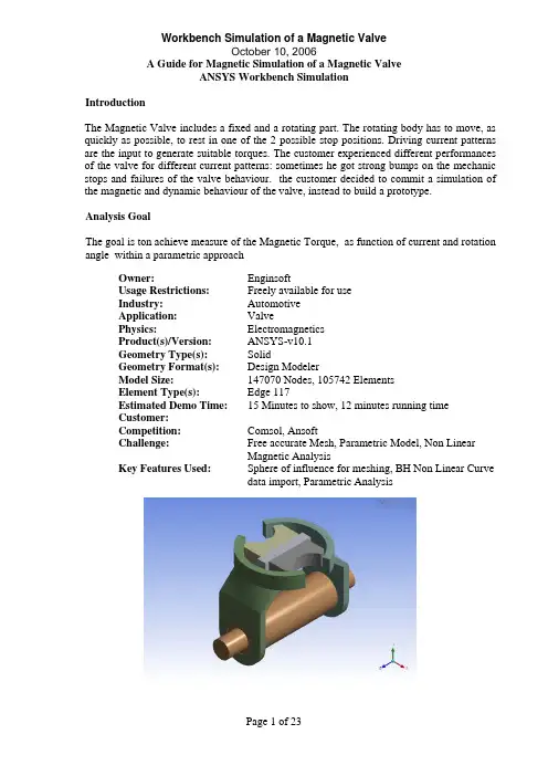
IntroductionThe Magnetic Valve includes a fixed and a rotating part. The rotating body has to move, as quickly as possible, to rest in one of the 2 possible stop positions. Driving current patterns are the input to generate suitable torques. The customer experienced different performances of the valve for different current patterns: sometimes he got strong bumps on the mechanic stops and failures of the valve behaviour. the customer decided to commit a simulation of the magnetic and dynamic behaviour of the valve, instead to build a prototype.Analysis GoalThe goal is ton achieve measure of the Magnetic Torque, as function of current and rotation angle within a parametric approachOwner:EnginsoftUsage Restrictions:Freely available for useIndustry:AutomotiveApplication:ValvePhysics:ElectromagneticsProduct(s)/Version:ANSYS-v10.1Geometry Type(s):SolidGeometry Format(s): Design ModelerModel Size:147070 Nodes, 105742 ElementsElement Type(s): Edge 117Estimated Demo Time:15 Minutes to show, 12 minutes running timeCustomer:Competition:Comsol,AnsoftChallenge:Free accurate Mesh, Parametric Model, Non LinearMagnetic AnalysisKey Features Used:Sphere of influence for meshing, BH Non Linear Curvedata import, Parametric AnalysisSteps and Points to Convey.Picture Guide.Start ANSYS Workbench Environment, and choose “New Geometry”.Importing of external geometrySet the desired length unit: meters.01) Click “File > Open > Import External Geometry File”.02) Click on “Generate” in order to confirm the importation of the geometry.The geometry regards a magnetic valve.Steps and Points to Convey.Picture Guide.Create a Parametric, Relative Rotation between two groups of bodies01) Create a local coordinate system (plane 4) by clicking on the “New Plane” icon in the tool bar.02) In “Details of Plane4 >. Type” choose from face in order to select the surface of interest. 03) Choose the space to the right of “Base Face” in Details of Plane4 and select the surface indicated in light blue in the plot at right.The local coordinate system “Plane 4” is now visible, centered on a face vertex04) In “Details of Plane4 >. Transform 1 (RMB)” insert an offset along X axis of –0.00825 m.05) In “Details of Plane4 >. Transform 1 (RMB)” insert an offset along Y axis of 0.0015 m.06) Click Generate to create Plane4Create another plane (Plane5).07) In “Details of Plane5 > Type” choose from plane. Base plane should be set to Plane4.08) In “Details of Plane5 >. Transform 1 (RMB)” insert a rotation about Z axis of 30°. 09) Click Generate to create Plane5.Steps and Points to Convey. Picture Guide.The local coordinate system “Plane 5” is now visible.10) From the tool bar menu, select “Tools > Freeze”.The freezing operation is indicated when bodies are displayed with transparency.11) From the tool bar menu, select “Create > Body Operation” set “Type” to “Move” click on the box to the right of Bodies.12) Select the bodies highlighted at right (use the Ctrl button to select multiple entities) and click Apply.Steps and Points to Convey.Picture Guide.13) In “Details of BodyOp1” choose the box to the right of “Source Plane” and pick on Plane4 in the Tree Outline.14) In a similar fashion, set “Destination Plane” to Plane5.Then click on “Generate” to move the parts as shown at right.ENCLOSURE definition01) From the tool bar menu, select “Tools >Enclosure” in order to insert a control volume cylindrically shaped and aligned to Y axis. Set the Cushion to 0.0375 m and set “Merge Parts?” to “Yes”.02) Click Generate to create the enclosureIn the “Outline” tree the just created enclosure is now visible.Steps and Points to Convey Picture GuideEnclosure is visible in the “Model View”window.CREATE the WINDING COIL01) In the Tree Outline, Open “1 Part, 7 Bodies > Part”. RMB on the last Solid in the list and choose “Hide Body” in the drop down menu. This will allow access to the surfaces of the imported geometry for forthcoming picking operations.02) Create a new plane (Plane6)03) In “Details of Plane6 >. Type” choose “From Face”.04) Click on the box to the right of “Base Face” and select the surface shown at right.05) In “Details of Plane6 >. Transform 1 (RMB)” insert an offset along Z axis of –0.0231 m.Click on Generate to create Plane6.06) With Plane6 now active, go to the tool bar and choose “New Sketch”.07) Select “Sketch1” in the “Tree Outline”.Steps and Points to Convey Picture Guide Sketching mode for winding coil generation08) Pick the Sketching tab at the bottom of theTree Outline09) Select “Circle” in the “Draw” window andchoose the center (origin of Plane6) and anarbitrary poin some distance away from thecenter to create a circle.10) Pick the Dimensions button at the bottom ofthe Sketching Toolboxes pane and choose“Radius”.11) Click on the circle and another arbitrarylocation for the radial dimension marker.12) In “Details of Sketch1”, modify the radiusR1 to be 0.00775 m.The sketch is now visible in the “Graphics”window.13) From the tool bar select “Concept > LineFrom Sketches”. Choose the circle and clickApply in the box to the right of “Base Objects”in “Details of Line1”. “Operation” should be setto “Add Material”.Click Generate.14) Choose the Line Body in the Tree Outline.15) In “Details of Line Body” set:•“Winding Body > Yes”•“Number of Turns” = 1•“CS Length” = 0.022 m•“CS Length” = 0.00375 mSteps and Points to ConveyPicture Guide16) From the tool bar, select “View > Show Cross Sections Solids”. The new winding body should appear as it does in the figure to the right.ANGLE as PARAMETER01) In the “Tree Outline” select “Plane5”02) Make the rotation about Z axis as parameter by clicking on the box to the left of “FD1, Value 1”.03) Rename the parameter as “angle”.Steps and Points to Convey.Picture Guide.04) From the tool bar, select “Tools > Options>Common Settings>Geometry Import”. Remove “DS” from the field to the right of “Personal Parameter Key” to remove the DS prefix naming convention restriction for importing parameters. Click OK.GO IN SIMULATIONIn the “[Project]” window, select “New Simulation”.In the “[Simulation]” window, the “Outline” tree should be as in figure.Steps and Points to ConveyPicture GuideMaterials Properties DefinitionSelect “Data” in the tool bar to open the “[Engineering Data]” window.Materials Properties Definitionchange defaults of STRUCTURAL STEEL01) Select “Structural Steel” and click on “Add/Remove Properties” in the “Electromagnetics” field and unselect the following items:- “Relative Permeability” - “Resistivity”02) Check the box to the left of “B-H curve” and click OK.03) Say “Yes” to the “Remove Material Properties” box that appears.04) Open excel file “bh1.xls” and copy the two data columns (highlight them with the mouse cursor and type Cntl-C).Steps and Points to ConveyPicture Guide05) Click the icon depicting an xy plot to the right of “B-H Curve”06) LMB on the 2 (second row) of the “Magnetic Flux Density vs. Magnetic Field Intensity” table and press “Ctrl +V” to paste the two column data from the .xls file.07) Click on the B-H Curve icon at the lower right.The curve should appear as shown at right.NEW Material definition IRONRMB on “Materials (2)” in the tree and choose “Insert New Material”. RMB on “New Material”, choose Rename and change the name of the new material to Iron. Define BH data as before but this time use data from “bh2.xls” file.NEW Material definition NEODYMIUM01) Define a New material named “Neodymium”.02) Among Electromagnetics properties let active just: “Linear Hard Material”: 03) Insert the following data:• Cohercive Force: 7.9577 e5 A/m • Residual Induction 1.2 T01) Return to the Simulation Tab02) In the Outline Tree, open Geometry>Part and use the Cntl button to select both of the RIC9512_105 items. The parts should be highlighted as shown at right.03) In Details of “Multiple Selection”, changematerial from “Structural Steel” to “Iron”Steps and Points to ConveyPicture Guide04) Select the part shown at right.05) Change material from “Structural Steel” to “Neodymium”MESH01) Select the coil support solid (see figure)02) RMB on “Mesh” on the tree to insert a sizing control: Element Size 2e-303) Insert another sizing control , 1e-3, referred to 5 bodies as in the following picture. It may help to hide the 4th solid (the “air enclosure) in the Outline tree to simplify selecting these parts.Steps and Points to ConveyPicture Guide5 bodies for sizing setting n.204) In the Outline tree, RMB on Model and insert a “Coordinate Systems” branch. RMB on the Coordinate Systems branch and insert (define) a new Coordinate System. Choose “Origin” in the Details of “Coordinate System” pane, select the surface shown at right, and click Apply.05) RMB on Mesh in the Outline to insert a third sizing control:For “Type”, choose “Sphere of Influence”• Sphere Center: Coordinate System (defined just before) • Radius 1.5e-2 • Element size 5e-4Areas to be applied are the following (10 areas)Steps and Points to ConveyPicture Guide10 Areas where to apply the Sphere of Influence sizing control06) Click on Mesh -> Preview MeshThe Mesh should result as in figure, if the “Air” solid enclosure body is hideLOADSSet the Conductor Current value in details window related to “Conductor Winding Body”: 1000 ABOUNDARY CONDITIONSRMB on Environment in the tree and insert a Magnetic Flux Parallel object. Use the Cntl button to select the 3 exterior surfaces of the enclosure and click Apply.Steps and Points to Convey.Picture Guide.POSTPROCESSING SETTINGS01) Insert under the “Solution” tree the following output requests: • Total Flux Density • Total Flux Intensity 02) Select 3 bodies as in figure03) Insert a “Directional Force/Torque” output request with details:• In Details of “Directional Force/Torque” pane, change “Global Coordinate System” to “Coordinate System” (this is the user-defined coordinate system centered on the top surface of the permanent magnet).• Set Orientation to Y Direction (rotation axis)04) repeat Directional Force/Torque Request for both X and Z axis direction05) By a right click under the Solution Tree Insert a “Solution Information” request to monitor the run during the solutionSOLVE01) Highlight the Environment tree tosee/check all Boundary & Loads previously defined.02) Click on the “SOLVE” Icon to launchthe run.Solution times takes about 12 minutes on a 2.8 Ghz single processor 32bit PCSteps and Points to ConveyPicture GuideREVIEW RESULTS01) See the Total Flux of Magnetic results 02) Set up a Vector Image of the MagneticField03) After Vector Image settings show a Vector Plot of Magnetic Field03)See the Magnetic Force distribution, Yaxis direction, on the requested parts. 04)The same for X, Z directions05)Activate the view from Y Global Axis06)Define a “Slice Plane”07)Draw the slice plane trace at nearlyalong the Y global direction08)View from the X Global direction09)Activate “show elements” and show themagnetic fieldSteps and Points to Convey Picture GuideSET UP A PARAMETRIC ANALYSIS01) Click on “Model”02) Click on CAD Parameters Detail toactivate the “angle” as a parameter. Thiswill be the first INPUT parameter.03) Click on Environment and Duplicate byright click04) Activate the Conductor Current Value asparameter. This is the second INPUTparameter n.2.05) Activate the Torque value in Y directionas OUTPUT parameter (ThirdParameter)06)Click on “Solution” of Environment 2and then click on Parameter Manager 07)Set up many cases as you like, forexample with 4 current values, 3 values other than the previously solved.。
ANSYS电磁场分析指南第一章磁场分析概述
第一章磁场分析概述1.1磁场分析对象利用ANSYS/Emag或ANSYS/Multiphysics模块中的电磁场分析功能,ANSYS 可分析计算下列的设备中的电磁场,如:·电力发电机·磁带及磁盘驱动器·变压器·波导·螺线管传动器·谐振腔·电动机·连接器·磁成像系统·天线辐射·图像显示设备传感器·滤波器·回旋加速器在一般电磁场分析中关心的典型的物理量为:·磁通密度·能量损耗·磁场强度·磁漏·磁力及磁矩· S-参数·阻抗·品质因子Q·电感·回波损耗·涡流·本征频率存在电流、永磁体和外加场都会激励起需要分析的磁场。
1.2ANSYS如何完成电磁场分析计算ANSYS以Maxwell方程组作为电磁场分析的出发点。
有限元方法计算的未知量(自由度)主要是磁位或通量,其他关心的物理量可以由这些自由度导出。
根据用户所选择的单元类型和单元选项的不同,ANSYS计算的自由度可以是标量磁位、矢量磁位或边界通量。
1.3静态、谐波、瞬态磁场分析利用ANSYS可以完成下列磁场分析:·2-D静态磁场分析,分析直流电(DC)或永磁体所产生的磁场,用矢量位方程。
参见本书“二维静态磁场分析”·2-D谐波磁场分析,分析低频交流电流(AC)或交流电压所产生的磁场,用矢量位方程。
参见本书“二维谐波磁场分析”·2-D瞬态磁场分析,分析随时间任意变化的电流或外场所产生的磁场,包含永磁体的效应,用矢量位方程。
参见本书“二维瞬态磁场分析”·3-D静态磁场分析,分析直流电或永磁体所产生的磁场,用标量位方法。
参见本书“三维静态磁场分析(标量位方法)”·3-D静态磁场分析,分析直流电或永磁体所产生的磁场,用棱边单元法。
ansys workbench电磁场仿真完整例子

IntroductionThe Magnetic Valve includes a fixed and a rotating part. The rotating body has to move, as quickly as possible, to rest in one of the 2 possible stop positions. Driving current patterns are the input to generate suitable torques. The customer experienced different performances of the valve for different current patterns: sometimes he got strong bumps on the mechanic stops and failures of the valve behaviour. the customer decided to commit a simulation of the magnetic and dynamic behaviour of the valve, instead to build a prototype.Analysis GoalThe goal is ton achieve measure of the Magnetic Torque, as function of current and rotation angle within a parametric approachOwner:EnginsoftUsage Restrictions:Freely available for useIndustry:AutomotiveApplication:ValvePhysics:ElectromagneticsProduct(s)/Version:ANSYS-v10.1Geometry Type(s):SolidGeometry Format(s): Design ModelerModel Size:147070 Nodes, 105742 ElementsElement Type(s): Edge 117Estimated Demo Time:15 Minutes to show, 12 minutes running timeCustomer:Competition:Comsol,AnsoftChallenge:Free accurate Mesh, Parametric Model, Non LinearMagnetic AnalysisKey Features Used:Sphere of influence for meshing, BH Non Linear Curvedata import, Parametric AnalysisSteps and Points to Convey.Picture Guide.Start ANSYS Workbench Environment, and choose “New Geometry”.Importing of external geometrySet the desired length unit: meters.01) Click “File > Open > Import External Geometry File”.02) Click on “Generate” in order to confirm the importation of the geometry.The geometry regards a magnetic valve.Steps and Points to Convey.Picture Guide.Create a Parametric, Relative Rotation between two groups of bodies01) Create a local coordinate system (plane 4) by clicking on the “New Plane” icon in the tool bar.02) In “Details of Plane4 >. Type” choose from face in order to select the surface of interest. 03) Choose the space to the right of “Base Face” in Details of Plane4 and select the surface indicated in light blue in the plot at right.The local coordinate system “Plane 4” is now visible, centered on a face vertex04) In “Details of Plane4 >. Transform 1 (RMB)” insert an offset along X axis of –0.00825 m.05) In “Details of Plane4 >. Transform 1 (RMB)” insert an offset along Y axis of 0.0015 m.06) Click Generate to create Plane4Create another plane (Plane5).07) In “Details of Plane5 > Type” choose from plane. Base plane should be set to Plane4.08) In “Details of Plane5 >. Transform 1 (RMB)” insert a rotation about Z axis of 30°. 09) Click Generate to create Plane5.Steps and Points to Convey. Picture Guide.The local coordinate system “Plane 5” is now visible.10) From the tool bar menu, select “Tools > Freeze”.The freezing operation is indicated when bodies are displayed with transparency.11) From the tool bar menu, select “Create > Body Operation” set “Type” to “Move” click on the box to the right of Bodies.12) Select the bodies highlighted at right (use the Ctrl button to select multiple entities) and click Apply.Steps and Points to Convey.Picture Guide.13) In “Details of BodyOp1” choose the box to the right of “Source Plane” and pick on Plane4 in the Tree Outline.14) In a similar fashion, set “Destination Plane” to Plane5.Then click on “Generate” to move the parts as shown at right.ENCLOSURE definition01) From the tool bar menu, select “Tools >Enclosure” in order to insert a control volume cylindrically shaped and aligned to Y axis. Set the Cushion to 0.0375 m and set “Merge Parts?” to “Yes”.02) Click Generate to create the enclosureIn the “Outline” tree the just created enclosure is now visible.Steps and Points to Convey Picture GuideEnclosure is visible in the “Model View”window.CREATE the WINDING COIL01) In the Tree Outline, Open “1 Part, 7 Bodies > Part”. RMB on the last Solid in the list and choose “Hide Body” in the drop down menu. This will allow access to the surfaces of the imported geometry for forthcoming picking operations.02) Create a new plane (Plane6)03) In “Details of Plane6 >. Type” choose “From Face”.04) Click on the box to the right of “Base Face” and select the surface shown at right.05) In “Details of Plane6 >. Transform 1 (RMB)” insert an offset along Z axis of –0.0231 m.Click on Generate to create Plane6.06) With Plane6 now active, go to the tool bar and choose “New Sketch”.07) Select “Sketch1” in the “Tree Outline”.Steps and Points to Convey Picture Guide Sketching mode for winding coil generation08) Pick the Sketching tab at the bottom of theTree Outline09) Select “Circle” in the “Draw” window andchoose the center (origin of Plane6) and anarbitrary poin some distance away from thecenter to create a circle.10) Pick the Dimensions button at the bottom ofthe Sketching Toolboxes pane and choose“Radius”.11) Click on the circle and another arbitrarylocation for the radial dimension marker.12) In “Details of Sketch1”, modify the radiusR1 to be 0.00775 m.The sketch is now visible in the “Graphics”window.13) From the tool bar select “Concept > LineFrom Sketches”. Choose the circle and clickApply in the box to the right of “Base Objects”in “Details of Line1”. “Operation” should be setto “Add Material”.Click Generate.14) Choose the Line Body in the Tree Outline.15) In “Details of Line Body” set:•“Winding Body > Yes”•“Number of Turns” = 1•“CS Length” = 0.022 m•“CS Length” = 0.00375 mSteps and Points to ConveyPicture Guide16) From the tool bar, select “View > Show Cross Sections Solids”. The new winding body should appear as it does in the figure to the right.ANGLE as PARAMETER01) In the “Tree Outline” select “Plane5”02) Make the rotation about Z axis as parameter by clicking on the box to the left of “FD1, Value 1”.03) Rename the parameter as “angle”.Steps and Points to Convey.Picture Guide.04) From the tool bar, select “Tools > Options>Common Settings>Geometry Import”. Remove “DS” from the field to the right of “Personal Parameter Key” to remove the DS prefix naming convention restriction for importing parameters. Click OK.GO IN SIMULATIONIn the “[Project]” window, select “New Simulation”.In the “[Simulation]” window, the “Outline” tree should be as in figure.Steps and Points to ConveyPicture GuideMaterials Properties DefinitionSelect “Data” in the tool bar to open the “[Engineering Data]” window.Materials Properties Definitionchange defaults of STRUCTURAL STEEL01) Select “Structural Steel” and click on “Add/Remove Properties” in the “Electromagnetics” field and unselect the following items:- “Relative Permeability” - “Resistivity”02) Check the box to the left of “B-H curve” and click OK.03) Say “Yes” to the “Remove Material Properties” box that appears.04) Open excel file “bh1.xls” and copy the two data columns (highlight them with the mouse cursor and type Cntl-C).Steps and Points to ConveyPicture Guide05) Click the icon depicting an xy plot to the right of “B-H Curve”06) LMB on the 2 (second row) of the “Magnetic Flux Density vs. Magnetic Field Intensity” table and press “Ctrl +V” to paste the two column data from the .xls file.07) Click on the B-H Curve icon at the lower right.The curve should appear as shown at right.NEW Material definition IRONRMB on “Materials (2)” in the tree and choose “Insert New Material”. RMB on “New Material”, choose Rename and change the name of the new material to Iron. Define BH data as before but this time use data from “bh2.xls” file.NEW Material definition NEODYMIUM01) Define a New material named “Neodymium”.02) Among Electromagnetics properties let active just: “Linear Hard Material”: 03) Insert the following data:• Cohercive Force: 7.9577 e5 A/m • Residual Induction 1.2 T01) Return to the Simulation Tab02) In the Outline Tree, open Geometry>Part and use the Cntl button to select both of the RIC9512_105 items. The parts should be highlighted as shown at right.03) In Details of “Multiple Selection”, changematerial from “Structural Steel” to “Iron”Steps and Points to ConveyPicture Guide04) Select the part shown at right.05) Change material from “Structural Steel” to “Neodymium”MESH01) Select the coil support solid (see figure)02) RMB on “Mesh” on the tree to insert a sizing control: Element Size 2e-303) Insert another sizing control , 1e-3, referred to 5 bodies as in the following picture. It may help to hide the 4th solid (the “air enclosure) in the Outline tree to simplify selecting these parts.Steps and Points to ConveyPicture Guide5 bodies for sizing setting n.204) In the Outline tree, RMB on Model and insert a “Coordinate Systems” branch. RMB on the Coordinate Systems branch and insert (define) a new Coordinate System. Choose “Origin” in the Details of “Coordinate System” pane, select the surface shown at right, and click Apply.05) RMB on Mesh in the Outline to insert a third sizing control:For “Type”, choose “Sphere of Influence”• Sphere Center: Coordinate System (defined just before) • Radius 1.5e-2 • Element size 5e-4Areas to be applied are the following (10 areas)Steps and Points to ConveyPicture Guide10 Areas where to apply the Sphere of Influence sizing control06) Click on Mesh -> Preview MeshThe Mesh should result as in figure, if the “Air” solid enclosure body is hideLOADSSet the Conductor Current value in details window related to “Conductor Winding Body”: 1000 ABOUNDARY CONDITIONSRMB on Environment in the tree and insert a Magnetic Flux Parallel object. Use the Cntl button to select the 3 exterior surfaces of the enclosure and click Apply.Steps and Points to Convey.Picture Guide.POSTPROCESSING SETTINGS01) Insert under the “Solution” tree the following output requests: • Total Flux Density • Total Flux Intensity 02) Select 3 bodies as in figure03) Insert a “Directional Force/Torque” output request with details:• In Details of “Directional Force/Torque” pane, change “Global Coordinate System” to “Coordinate System” (this is the user-defined coordinate system centered on the top surface of the permanent magnet).• Set Orientation to Y Direction (rotation axis)04) repeat Directional Force/Torque Request for both X and Z axis direction05) By a right click under the Solution Tree Insert a “Solution Information” request to monitor the run during the solutionSOLVE01) Highlight the Environment tree tosee/check all Boundary & Loads previously defined.02) Click on the “SOLVE” Icon to launchthe run.Solution times takes about 12 minutes on a 2.8 Ghz single processor 32bit PCSteps and Points to ConveyPicture GuideREVIEW RESULTS01) See the Total Flux of Magnetic results 02) Set up a Vector Image of the MagneticField03) After Vector Image settings show a Vector Plot of Magnetic Field03)See the Magnetic Force distribution, Yaxis direction, on the requested parts. 04)The same for X, Z directions05)Activate the view from Y Global Axis06)Define a “Slice Plane”07)Draw the slice plane trace at nearlyalong the Y global direction08)View from the X Global direction09)Activate “show elements” and show themagnetic fieldSteps and Points to Convey Picture GuideSET UP A PARAMETRIC ANALYSIS01) Click on “Model”02) Click on CAD Parameters Detail toactivate the “angle” as a parameter. Thiswill be the first INPUT parameter.03) Click on Environment and Duplicate byright click04) Activate the Conductor Current Value asparameter. This is the second INPUTparameter n.2.05) Activate the Torque value in Y directionas OUTPUT parameter (ThirdParameter)06)Click on “Solution” of Environment 2and then click on Parameter Manager 07)Set up many cases as you like, forexample with 4 current values, 3 values other than the previously solved.。
ANSYS有限元案例分析之磁场分布仿真案例
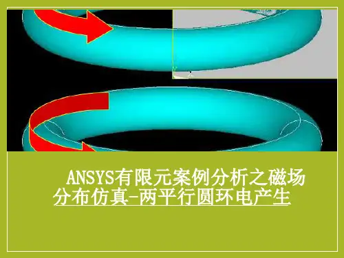
ANSYS有限元案例分析-两平行圆环电产生磁场分布仿真
二,前处理
•3 创建模型
2)生成四分之一圆,圆心(0,0)半径20: Main Menu:Preprocessor>Modeling>Create
>Areas>Circle>Partial Annulus。Rad-1 输入20 ;Theta-2输入90;点击OK。
中选择Axisymmetric;同理选择type2做如上操作。
ANSYS有限元案例分析-两平行圆环电产生磁场分布仿真
一,前处理
• 2定义材料特性
1)相对磁导率 Main Menu: Preprocessor > Material Props >Relative Permeability>Constant
ANSYS有限元案例分析之磁场 分布仿真-两平行圆环电产生
ANSYS有限元案例分析-两平行圆环电产生磁场分布仿真
一,前处理前的操作
•1 文件路径,工作名称和工作标题的设定。
1)文件路径:Utility Menu:File>Change Directory 2)工作名称:Utility Menu:File>Change Jobname 3)工作标题:Utility Menu:File>Change Title
ANSYS有限元案例分析-两平行圆环电产生磁场分布仿真
四,求解
• 7 往路径上映射变量的数值: Main Menu>General Postproc>Path Operation>Map onto Path。左边一栏选择Flux&gradient,右边选择 MagFluxDens BSUM,点击OK。
AnsysMaxwell在工程电磁场中的应用1——二维分析技术
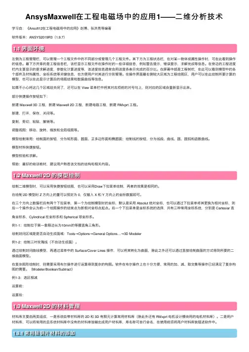
AnsysMaxwell在⼯程电磁场中的应⽤1——⼆维分析技术学习⾃:《Ansoft12在⼯程电磁场中的应⽤》赵博、张洪亮等编著软件版本:ANSYS2019R3(1.9.7)1.1 界⾯环境左侧为⼯程管理栏,可以管理⼀个⼯程⽂件中的不同部分或管理⼏个⼯程⽂件。
其下⽅为⼯程状态栏,在对某⼀物体或属性操作时,可在此看到操作的信息。
最下⽅并排的是⼯程信息栏,该栏显⽰⼯程⽂件在操作时的⼀些详细信息,例如警告提⽰,错误提⽰,求解完成等信息。
在旁边的⼯程进度栏内主要显⽰的是求解进度,参数化计算进度等,该进度信息通常会⽤进度条表⽰完成的百分⽐。
在屏幕中部是⼯程树栏,在此可以看到模型中的各个部件及材料属性、坐标系统等关键信息,也⽅便⽤户对其进⾏分别管理。
在操作界⾯最右侧较⼤区域为⼯程绘图区,⽤户可以在此绘制所要计算的模型,也可以在此显⽰计算后的场图结果和数据曲线等信息。
如果不⼩⼼将这⼏个区域给关闭了,还可以在 View 菜单栏中将其对应项前的对号勾上,则对应的区域会重新显⽰出来。
部分快捷操作按钮如下:新建 Maxwell 3D ⼯程,新建 Maxwell 2D ⼯程,新建电路⼯程,新建 RMxprt ⼯程。
新建,打开,保存,关闭等。
复制,剪切,粘贴,撤销等。
调整视图:移动、旋转、缩放和全局视图等。
模型绘制常⽤:绘制⾯的按钮,分为矩形⾯、圆⾯、正多边形⾯和椭圆⾯;绘制线的按钮,分为线段、曲线、圆、圆弧和函数曲线。
模型材料快捷按钮。
模型校验和求解。
帮助:最好的培训教材,建议⽤户熟悉该⽂档的结构和相关内容。
1.2 Maxwell 2D 的模型绘制绘制⼆维模型时,可以采⽤快捷按钮绘图,也可以采⽤Draw下拉菜单绘制,两者的效果是相同的。
在绘制 2D 模型时 Z ⽅向上的量可以恒定为 0,仅输⼊ X 和 Y ⽅向上的坐标数据即可。
在三个⽅向上数据栏后有两个下拉菜单,第⼀个为绘制模型时的坐标,默认是采⽤ Absolut 绝对坐标,也可以通过下拉菜单将其更换为相对坐标,则后⼀个操作会认为前⼀个绘图操作的结束点为新相对坐标点起点。
ANSYS_Workbench_电磁场分析例子

– Simulation
© 2004 ANSYS, Inc.
ANSYS, Inc. Proprietary
Winding Bodies & Tool
• Feature: Design Modeler (DM) includes two new tools to allow a user to easily create current carrying coils: – Winding Bodies: Used to represent wound coils for source excitation. The advantage of these bodies is that they are not 3D CAD objects, and hence simplify modeling/meshing of winding structures. – Upon “attach to Simulation”, Winding Bodies are assigned as Conductor bodies. – Winding Tool: Used to create more complex coils for motor windings. The Winding Tool uses a Worksheet table format to drive the creation of multiply connected Winding Bodies. Or a user can read in a text file created by MSExcel.
ANSYS Workbench 9.0 Electromagnetics
Paul Lethbridge
© 2004 ANSYS, Inc.
ANSYSWorkbench电磁场分析例子共38页
ANSYS, Inc. Proprietary
Contents
Workbench Electromagnetics
– Workbench Emag Roadmap
– Design Modeler
• Enclosure Symmetry • Winding bodies • Winding Tool
• Workbench v9.0 is the first release with electromagnetic analysis capability. – Support solid and stranded (wound) conductors – Automated computations of force, torque, inductance, and coil flux linkage. – Easily set up simulations to compute results as a function of current, stroke, or rotor angle.
– Up to 3 three symmetry planes can be specified. – Full or partial models can be included in the Enclosure. – During the model transfer from DesignModeler to Simulation, the enclosure feature with symmetry planes forms two kinds of named selections:
– Winding Bodies: Used to represent wound coils for source excitation. The advantage of these bodies is that they are not 3D CAD objects, and hence simplify modeling/meshing of winding structures.
ANSYS电磁场教程电磁模拟
THANKS FOR WATCHING
感谢您的观看
03Байду номын сангаас
本文介绍了ANSYS电磁场教程的基本内容和应用实例,包括静电场、静磁场和 时变电磁场的模拟分析,旨在帮助读者更好地理解和掌握ANSYS在电磁场分析 中的应用。
展望
随着科技的不断进步和应用需求的不断增加,电磁模拟技 术将越来越受到重视,ANSYS作为该领域的领先软件,将 继续发挥重要作用。
未来,ANSYS将不断更新和完善其功能和工具,以更好地 满足用户的需求,包括提高模拟精度、增加新的分析模块 和优化计算效率等。
后处理
分析结果、可视化展示等。
03 电磁场模拟案例分析
案例一:简单电场模拟
建立模型
创建一个简单的二维电场模型, 包括两个电极板和空气区域。
求解设置
选择合适的求解器类型和迭代 次数,进行电场模拟。
总结词
通过ANSYS软件进行简单电场 模拟,了解电场分布和电势分 布。
边界条件
设置电极板为电势边界条件, 设置空气区域为零电势边界条 件。
结果分析
查看电场分布云图和电势分布 云图,分析电场强度和电势的 变化趋势。
案例二:磁场模拟
总结词
通过ANSYS软件进 行磁场模拟,了解磁 场分布和磁感应强度 分布。
建立模型
创建一个简单的三维 磁场模型,包括一个 永磁体和空气区域。
边界条件
设置永磁体为磁化方 向边界条件,设置空 气区域为零磁感应强 度边界条件。
结果分析实例
磁场分布
通过后处理技术,将模拟得 到的磁场分布进行可视化展 示,并与理论值进行对比分 析。
ANSYSWorkbench电磁场分析例子
Paul Lethbridge
© 2004 ANSYS, Inc.
ANSYS, Inc. Proprietary
Contents
Workbench Electromagnetics
– Workbench Emag Roadmap
– Design Modeler
• Enclosure Symmetry • Winding Bodies • Winding Tool
– Simulation
© 2004 ANSYS, Inc.
ANSYS, Inc. Proprietary
Workbench Emag Roadmap
• LF Emag capability will be exposed over several release cyc – 3D Current conduction (10.0) – 3D Electrostatics Circuit elements – Time transient & 2D
ANSYS, Inc. Proprietary
Fill Feature
• The Fill feature create a new frozen body to fill the space occupied by a hole or cavity.
• Useful for interior cavity electromagnetic applications.
• Enclosure tool: Released at 8.0. This tool is used to completely enclose the bodies of a model in a material typically required for an Emag analysis.
ansysworkbench电磁场仿真完整例子
IntroductionThe Magnetic Valve includes a fixed and a rotating part. The rotating body has to move, as quickly as possible, to rest in one of the 2 possible stop positions. Driving current patterns are the input to generate suitable torques. The customer experienced different performances of the valve for different current patterns: sometimes he got strong bumps on the mechanic stops and failures of the valve behaviour. the customer decided to commit a simulation of the magnetic and dynamic behaviour of the valve, instead to build a prototype.Analysis GoalThe goal is ton achieve measure of the Magnetic Torque, as function of current and rotation angle within a parametric approachOwner:EnginsoftUsage Restrictions:Freely available for useIndustry:AutomotiveApplication:ValvePhysics:ElectromagneticsProduct(s)/Version:ANSYS-v10.1Geometry Type(s):SolidGeometry Format(s): Design ModelerModel Size:147070 Nodes, 105742 ElementsElement Type(s): Edge 117Estimated Demo Time:15 Minutes to show, 12 minutes running timeCustomer:Competition:Comsol, AnsoftChallenge:Free accurate Mesh, Parametric Model, Non LinearMagnetic AnalysisKey Features Used:Sphere of influence for meshing, BH Non Linear Curvedata import, Parametric AnalysisSteps and Points to Convey. Picture Guide. Start ANSYS Workbench Environment, andchoose “New Geometry”.Importing of external geometrySet the desired length unit: meters.01) Click “File > Open > Import ExternalGeometry File”.02) Click on “Generate” in order to confirm theimportation of the geometry.The geometry regards a magnetic valve.Steps and Points to Convey. Picture Guide. Create a Parametric, Relative Rotationbetween two groups of bodies01) Create a local coordinate system (plane 4)by clicking on the “New Plane” icon in the toolbar.02) In “Details of Plane4 >. Type” choose fromface in order to select the surface of interest.03) Choose the space to the right of “Base Face” in Details of Plane4 and select the surfaceindicated in light blue in the plot at right.The local coordinate system “Plane 4” is nowvisible, centered on a face vertex04) In “Details of Plane4 >. Transform 1(RMB)” insert an offset along X axis of –0.00825 m.05) In “Details of Plane4 >. Transform 1(RMB)” insert an offset along Y axis of 0.0015m.06) Click Generate to create Plane4Create another plane (Plane5).07) In “Details of Plane5 > Type” choose fromplane. Base plane should be set to Plane4.08) In “Details of Plane5 >. Transform 1(RMB)” insert a rotation about Z axis of 30°.09) Click Generate to create Plane5.Steps and Points to Convey. Picture Guide. The local coordinate system “Plane 5” is nowvisible.10) From the tool bar menu, select “Tools >Freeze”.The freezing operation is indicated when bodiesare displayed with transparency.11) From the tool bar menu, select “Create >Body Operation” set “Type” to “Move” click onthe box to the right of Bodies.12) Select the bodies highlighted at right (usethe Ctrl button to select multiple entities) andclick Apply.Steps and Points to Convey. Picture Guide.13) In “Details of BodyOp1” choose the box tothe right of “Source Plane” and pick on Plane4in the Tree Outline.14) In a similar fashion, set “Destination Plane” to Plane5.Then click on “Generate” to move the parts asshown at right.ENCLOSURE definition01)From the tool bar menu, select “Tools >Enclosure” in order to insert a controlvolume cylindrically shaped and alignedto Y axis. Set the Cushion to 0.0375 mand set “Merge Parts?” to “Yes”.02)Click Generate to create the enclosureIn the “Outline” tree the just created enclosure isnow visible.Steps and Points to Convey Picture Guide Enclosure is visible in the “Model View” window.CREATE the WINDING COIL01) In the Tree Outline, Open “1 Part, 7 Bodies> Part”. RMB on the last Solid in the list andchoose “Hide Body” in the drop down menu.This will allow access to the surfaces of theimported geometry for forthcoming pickingoperations.02) Create a new plane (Plane6)03) In “Details of Plane6 >. Type” choose“From Face”.04) Click on the box to the right of “Base Face” and select the surface shown at right.05) In “Details of Plane6 >. Transform 1(RMB)” insert an offset along Z axis of –0.0231 m.Click on Generate to create Plane6.06) With Plane6 now active, go to the tool barand choose “New Sketch”.07) Select “Sketch1” in the “Tree Outline”.Steps and Points to Convey Picture Guide Sketching mode for winding coil generation08) Pick the Sketching tab at the bottom of theTree Outline09) Select “Circle” in the “Draw” window andchoose the center (origin of Plane6) and anarbitrary poin some distance away from thecenter to create a circle.10) Pick the Dimensions button at the bottom ofthe Sketching Toolboxes pane and choose“Radius”.11) Click on the circle and another arbitrarylocation for the radial dimension marker.12) In “Details of Sketch1”, modify the radiusR1 to be 0.00775 m.The sketch is now visible in the “Graphics” window.13) From the tool bar select “Concept > LineFrom Sketches”. Choose the circle and clickApply in the box to the right of “Base Objects” in “Details of Line1”. “Operation” should be setto “Add Material”.Click Generate.14) Choose the Line Body in the Tree Outline.15) In “Details of Line Body” set:?“Winding Body > Yes” ?“Number of Turns” = 1?“CS Length” = 0.022 m?“CS Length” = 0.00375 mSteps and Points to Convey Picture Guide 16) From the tool bar, select “View > ShowCross Sections Solids”. The new winding bodyshould appear as it does in the figure to the right.ANGLE as PARAMETER01) In the “Tree Outline” select “Plane5” 02) Make the rotation about Z axis as parameterby clicking on the box to the left of “FD1, Value1”.03) Rename the parameter as “angle”.Steps and Points to Convey. Picture Guide.04) From the tool bar, select “Tools >Options>Common Settings>Geometry Import”.Remove “DS” from the field to the right of“Personal Parameter Key” to remove the DSprefix naming convention restriction forimporting parameters. Click OK.GO IN SIMULATIONIn the “[Project]” window, select “NewSimulation”.In the “[Simulation]” window, the “Outline” treeshould be as in figure.Steps and Points to Convey Picture GuideMaterials Properties DefinitionSelect “Data” in the tool bar to open the“[Engineering Data]” window.Materials Properties Definitionchange defaults of STRUCTURAL STEEL01) Select “Structural Steel” and click on“Add/Remove Properties” in the“Electromagnetics” field and unselect thefollowing items:-“Relative Permeability” -“Resistivity” 02) Check the box to the left of “B-H curve” andclick OK.03) Say “Yes” to the “Remove MaterialProperties” box that appears.04) Open excel file “bh1.xls” and copy the twodata columns (highlight them with the mousecursor and type Cntl-C).Steps and Points to Convey Picture Guide 05) Click the icon depicting an xy plot to theright of “B-H Curve”06) LMB on the 2 (second row) of the“Magnetic Flux Density vs. Magnetic FieldIntensity” table and press “Ctrl +V” to paste thetwo column data from the .xls file.07) Click on the B-H Curve icon at the lowerright.The curve should appear as shown at right.NEW Material definition IRONRMB on “Materials (2)” in the tree and choose“Insert New Material”. RMB on “NewMaterial”, choose Rename and change the nameof the new material to Iron. Define BH data asbefore but this time use data from “bh2.xls” file.NEW Material definition NEODYMIUM01) Define a New material named“Neodymium”.02) Among Electromagnetics properties letactive just: “Linear Hard Material”:03) Insert the following data:?Cohercive Force: 7.9577 e5 A/m?Residual Induction 1.2 TAssign MAT PROPS to parts01) Return to the Simulation Tab02) In the Outline Tree, open Geometry>Partand use the Cntl button to select both of theRIC9512_105 items. The parts should behighlighted as shown at right.03) In Details of “Multiple Selection”, change material from “Structural Steel” to “Iron” Steps and Points to Convey Picture Guide04) Select the part shown at right.05) Change material from “Structural Steel” to “Neodymium” MESH01) Select the coil support solid (see figure)02) RMB on “Mesh” on the tree to insert asizing control:Element Size 2e-303) Insert another sizing control , 1e-3, referredto 5 bodies as in the following picture. It mayhelp to hide the 4th solid (the “air enclosure) inthe Outline tree to simplify selecting these parts.Steps and Points to Convey Picture Guide 5 bodies for sizing setting n.204) In the Outline tree, RMB on Model andinsert a “Coordinate Systems” branch. RMB onthe Coordinate Systems branch and insert(define) a new Coordinate System. Choose“Origin” in the Details of “Coordinate System” pane, select the surface shown at right, and clickApply.05) RMB on Mesh in the Outline to insert a thirdsizing control:For “Type”, choose “Sphere of Influence” ?Sphere Center: Coordinate System(defined just before)?Radius 1.5e-2?Element size 5e-4Areas to be applied are the following (10 areas)Steps and Points to Convey Picture Guide 10 Areas where to apply the Sphere of Influencesizing control06) Click on Mesh -> Preview MeshThe Mesh should result as in figure, if the “Air” solid enclosure body is hideLOADSSet the Conductor Current value in detailswindow related to “Conductor Winding Body”:1000 ABOUNDARY CONDITIONSRMB on Environment in the tree and insert aMagnetic Flux Parallel object. Use the Cntlbutton to select the 3 exterior surfaces of theenclosure and click Apply.Steps and Points to Convey. Picture Guide.POSTPROCESSING SETTINGS01) Insert under the “Solution” tree thefollowing output requests:?Total Flux Density?Total Flux Intensity02) Select 3 bodies as in figure03) Insert a “Directional Force/Torque” outputrequest with details:?In Details of “Directional Force/Torque” pane, change “Global CoordinateSystem” to “Coordinate System” (this isthe user-defined coordinate systemcentered on the top surface of thepermanent magnet).?Set Orientation to Y Direction (rotationaxis)04) repeat Directional Force/Torque Requestfor both X and Z axis direction05) By a right click under the Solution TreeInsert a “Solution Information” request tomonitor the run during the solutionSOLVE01)Highlight the Environment tree tosee/check all Boundary & Loadspreviously defined.02)Click on the “SOLVE” Icon to launchthe run.Solution times takes about 12 minutes on a 2.8 Ghz single processor 32bit PCSteps and Points to Convey Picture GuideREVIEW RESULTS01)See the Total Flux of Magnetic results02)Set up a Vector Image of the MagneticField03) After Vector Image settings show aVector Plot of Magnetic Field03)See the Magnetic Force distribution, Yaxis direction, on the requested parts.04)The same for X, Z directions05)Activate the view from Y Global Axis06)Define a “Slice Plane” 07)Draw the slice plane trace at nearlyalong the Y global direction08)View from the X Global direction09)Activate “show elements” and show themagnetic fieldSteps and Points to Convey Picture GuideSET UP A PARAMETRIC ANALYSIS01)Click on “Model” 02)Click on CAD Parameters Detail toactivate the “angle” as a parameter. Thiswill be the first INPUT parameter.03)Click on Environment and Duplicate byright click04)Activate the Conductor Current Value asparameter. This is the second INPUTparameter n.2.05)Activate the Torque value in Y directionas OUTPUT parameter (ThirdParameter)06)Click on “Solution” of Environment 2and then click on Parameter Manager07)Set up many cases as you like, forexample with 4 current values, 3 valuesother than the previously solved.。
- 1、下载文档前请自行甄别文档内容的完整性,平台不提供额外的编辑、内容补充、找答案等附加服务。
- 2、"仅部分预览"的文档,不可在线预览部分如存在完整性等问题,可反馈申请退款(可完整预览的文档不适用该条件!)。
- 3、如文档侵犯您的权益,请联系客服反馈,我们会尽快为您处理(人工客服工作时间:9:00-18:30)。
2.1-1 2.2-1 2.3-1 2.4-1 2.5-1
3.1-1 3.2-1
4.1-1 4.2-1 4.3-1 4.4-1 4.5-1 5-1
第一章
教程综述
• • •
ANSYS/EMAG能用于模拟工业电磁装 能用于模拟工业电磁装 置 电磁装置当然是3维 电磁装置当然是 维,但可简化 为2维模 维模 型。 模拟可考虑为: 模拟可考虑为: – 稳态 – 交流(谐波) 交流(谐波) – 时变瞬态 • 阶跃电压 • PWM(脉宽调制) 脉宽调制) 脉宽调制 (Pulse Width Modulation) • 任意
目录
第一章 电磁场仿真简介……………………………………….... 电磁场仿真简介……………………………………….... …….... …….... …….... …….... 第二章 二维静态分析 1节 第1节……………………………………………………………………………..… 第2节……………………………………………………………….……….……… 节 第3节…………………………………………………………………….….……… 节 第4节…………………………………………………………………………..…… 节 第5节……………………………………………………………………………..… 节 第三章 二维谐波和瞬态分析 第1节…………………………………………………………………………….…. 节 第2节…………………………………………………………………...………….. 节 第四章 三维电磁场分析 第1节…………………………………………………………………………...….… 节 第2节…………………………………………………………………….……….... 节 第3节………………………………………………………………….…..…….…. 节 第4节………………………………………………………………….……...……. 节 第5节…………………………………………………………………….…...……. 节 第五章 耦合场分析概况…………………………………………………………………………….. ………………………………………………子设计 致动器的一个实例 – 衔铁旋转 – 衔铁气隙可变化 完整模型由2个独立部件组成 完整模型由 个独立部件组成 – 衔铁模块 – 定子模块
•
执行: 执行 solen3d.avi看动画 看动画
模拟过程概述
• 利用如下方式观察装置 – 2D与3D 与 – 平面与轴对称 – 利用轴对称平面简化模型 定义物理区域 – 空气,铁,永磁体等等 空气, – 绞线圈,块导体 绞线圈, – 短路,开路 短路, 为每个物理区定义材料 – 导磁率(常数或非线性) 导磁率(常数或非线性) – 电阻率 – 矫顽磁力,剩余磁感应 矫顽磁力, 衔铁
•
• 在叠片条件下,利用磁通密度计算铁芯损失特定实例(以铁芯损失密度数 在叠片条件下,利用磁通密度计算铁芯损失特定实例( 据表示) 据表示)
叠片铁心 损耗数据
磁通密度
铁损 (W)
•
线圈
锭子 实体模型
•
• • •
建实体模型 给模型赋予属性以模拟物理区 赋予边界条件 – 线圈激励 – 外部边界 – 开放边界 实体模型划分网格 加补充约束条件(如果有必要) 加补充约束条件(如果有必要) – 周期性边界条件 – 连接不同网格 有限元网格
• •
• •
进行模拟 观察结果 – 某指定时刻 – 整个时间历程 后处理 – 磁力线 – 力 – 力矩 – 损耗 – MMF(磁动势) (磁动势) – 电感 – 特定需要