(完整)ANSYS传热分析实例汇总,推荐文档
ANSYS之杯具热分析
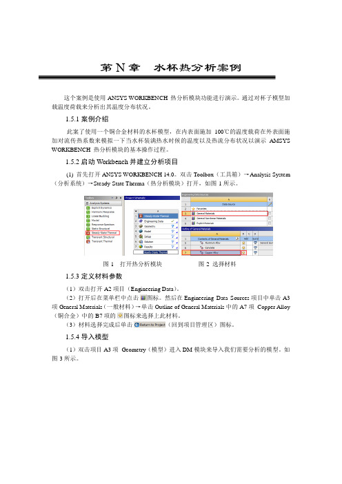
第N章水杯热分析案例这个案例是使用ANSYS WORKBENCH 热分析模块功能进行演示。
通过对杯子模型加载温度荷载来分析出其温度分布状况。
1.5.1案例介绍此案了使用一个铜合金材料的水杯模型,在内表面施加100℃的温度载荷在外表面施加对流传热系数来模拟一下当水杯装满热水时候的温度以及热流分布状况以演示AMSYS WORKBENCH 热分析模块的基本操作过程。
1.5.2启动Workbench并建立分析项目(1) 首先打开ANSYS WORKBENCH 14.0。
双击Toolbox(工具箱)→Analysis System (分析系统)→Steady-State Therma(热分析模块)打开,如图-1所示。
图-1 打开热分析模块图-2 选择材料1.5.3定义材料参数(1)双击打开A2项目(Engineering Data)。
(2)打开后在菜单栏中点击图标。
然后在Engineering Data Sources项目中单击A3项General Materials(一般材料)→单击Outline of General Materials中的A7项Copper Alloy(铜合金)中的B7项的图标来选择上此材料。
(3)材料选择完成后单击(回到项目管理区)图标。
1.5.4导入模型(1)双击项目A3项Geometry(模型)进入DM模块来导入我们需要分析的模型。
如图-3所示。
图-3 打开DM模块图-5 导入模型(2)单击File(文件)→Import External Geometry File(导入模型文件)。
如图-5所示。
(3)找到模型文件单击选择后单击“打开”按钮。
如图-6所示。
图-6 打开模型图-7 划分网格1.5.5划分网格(1)双击项目文件A4项Model(网格)。
如图-7所示。
打开的模型如图-8所示。
图-8 杯子的模型图-9 刷新网格(2)我们先使用程序自动划分网格,通过查看网格质量再决定是否进行网格控制。
ansys瞬态热分析教程及实例
大家好
QUST
18
自动时间步长选项 命令:AUTOTS GUI:Main Menu > Solution > Analysis Type
> Sol'n Controls 打开后求解过程中将自动调整时间步长。
大家好
QUST
19
时间积分选项 命令:TIMINT GUI:Main Menu > Solution > Load Step
QUST
6
大家好
5. 瞬态传热分析
均匀初始温度:如果整个模
型的初始温度为均匀且非0
2
,使用下列菜单指定:
3 4 1
QUST
7
大家好
1
2 3
5. 瞬态传热分析
非均匀的初始温度
如果模型的初始温度分布
已知但不均匀,使用这些
菜单将初始条件施加在特
4
定节点上
5
QUST
8
大家好
5. 瞬态传热分析
ANSYS 瞬态传热分析的主要步骤 1.建立有限元模型 2.施加载荷并求解 3.求解 4.查看分析结果
QUST
5
大家好
5. 瞬态传热分析
在瞬态分析中,载荷步和子步的定义与非线性稳态分 析十分类似。载荷定义的每个载荷步的终点,并可以 随时间阶跃或渐进的施加。
每个载荷步的求解是在子步上得到。子步长根据时间 积分步长得到。
自动时间步 (ATS) 同样适用于瞬态分析,可以简化 ITS选择。 ITS选择将影响到瞬态分析的精度和非线性收敛性 (如果存在)。
Restart
大家好
QUST
10条件分为两种情况:其一, 初始温度场已知;其二,初始温度场未知。
Ansys 共轭传热分析实例

图3操作项设置面板
设置流体域介质为air,固体域介质为默认的AL。
按图1所示边界条件设置计算域边界。
创建交界面,如图4所示进行设置。
图4设置交界面
4、初始化计算
设置初始化温度293K,如图5所示。
图5初始化面板
设置自动保存选项与动画录制项。
设置时间步长0.1s,时间步数100,内迭代次数20
图5简化模型
图6仿真模型
这幅图中可以看得更清楚,经过模型简化后,流体部分的外轮廓线是比较简洁的。注意这部分必须与齿轮箱贴合,这样以后计算热固耦合的时候,可以传递这个面上的温度场数据,如下图所示。这部分内容本帖中不涉及,本案例在流体外部用fluent的虚拟壁厚技术模拟一个壳体。
一些基础几何参数:
图7仿真模型与箱体示意图
我们首先来分析齿轮箱的结构,齿轮箱机械结构由壳体、端盖、大小齿轮、轴承、轴以及其他附件构成,我们首先要搞清楚分析的对象。壳体的温度是否是我们关注的要点?在本例中不是,那么我们的分析对象就是壳体中的所有元素,壳体只作为仿真的外边界。轴承和轴在仿真中的意义也不明显,因此我们都予以简化。
分析传热模型,齿轮摩擦生热是热源,这些热量通过几种方式传播:
网格划分完毕的效果如图:
图9整体网格
图10 局部网格
以上网格都是四面体单元,方便进行动网格设置。如不要求精确解,我们可以减小网格数目,采取以下这种单元数目较少的网格。可以看出,body之间的网格节点不共享。
图11简化网格
一些和网格划分有关的细节,可以按照这个表格去进行具体设置。这里的Advanced sizing功能一定要打开,否则在边角处生成的网格质量很差。表中用颜色标出了影响较大的设置项。
共轭传热计算
ansys瞬态热分析教程及实例
命令:ET,1,PLANE55
大家好
QUST
26
(2) 定义材料属性
首先进入Define Material Model Behavior 对话框,操作如下:
GUI:Main Menu > Preprocessor > Material Props
命令:TIME GUI:Main Menu > Solution > Analysis Type >
Sol'n Controls > basic 4)写入载荷步文件 命令:LSWRITE GUI:Main Menu > Solution > Load Step Opts >
Write LS File 或先求解:
大家好
QUST
37
(2)定义初始条件
板的初始温度为20℃,设置初始温度操作 如下:
GUI:Main Menu > Solution > Define Loads > Apply > Initial Condit'n > Define
在弹出的拾取对话框中,单击Pick All。弹 出Define Initial Conditions对话框,
14
3. 设定非均匀的初始温度 命令:IC GUI:Main Menu > Solution > Define Loads
> Apply > Initial Condit'n > Define
在瞬态传热分析中,节点温度可以通过此项设 定为不同的值。
大家好
QUST
(最新整理)ANSYS热分析详解
(完整)ANSYS热分析详解编辑整理:尊敬的读者朋友们:这里是精品文档编辑中心,本文档内容是由我和我的同事精心编辑整理后发布的,发布之前我们对文中内容进行仔细校对,但是难免会有疏漏的地方,但是任然希望((完整)ANSYS热分析详解)的内容能够给您的工作和学习带来便利。
同时也真诚的希望收到您的建议和反馈,这将是我们进步的源泉,前进的动力。
本文可编辑可修改,如果觉得对您有帮助请收藏以便随时查阅,最后祝您生活愉快业绩进步,以下为(完整)ANSYS热分析详解的全部内容。
第一章简介一、热分析的目的热分析用于计算一个系统或部件的温度分布及其它热物理参数,如热量的获取或损失、热梯度、热流密度(热通量〕等。
热分析在许多工程应用中扮演重要角色,如内燃机、涡轮机、换热器、管路系统、电子元件等。
二、ANSYS的热分析•在ANSYS/Multiphysics、ANSYS/Mechanical、ANSYS/Thermal、ANSYS/FLOTRAN、ANSYS/ED五种产品中包含热分析功能,其中ANSYS/FLOTRAN不含相变热分析。
•ANSYS热分析基于能量守恒原理的热平衡方程,用有限元法计算各节点的温度,并导出其它热物理参数。
•ANSYS热分析包括热传导、热对流及热辐射三种热传递方式.此外,还可以分析相变、有内热源、接触热阻等问题。
三、ANSYS 热分析分类•稳态传热:系统的温度场不随时间变化•瞬态传热:系统的温度场随时间明显变化四、耦合分析•热-结构耦合•热-流体耦合•热-电耦合•热-磁耦合•热-电-磁-结构耦合等第二章 基础知识一、符号与单位 W/m 2—℃ 二、传热学经典理论回顾热分析遵循热力学第一定律,即能量守恒定律:● 对于一个封闭的系统(没有质量的流入或流出〕PE KE U W Q ∆+∆+∆=-式中: Q —— 热量;W -- 作功;∆U ——系统内能;∆KE ——系统动能;∆PE —-系统势能;●对于大多数工程传热问题:0==PE KE ∆∆; ●通常考虑没有做功:0=W , 则:U Q ∆=; ● 对于稳态热分析:0=∆=U Q ,即流入系统的热量等于流出的热量;●对于瞬态热分析:dt dU q =,即流入或流出的热传递速率q 等于系统内能的变化。
ANSYS热分析指南——ANSYS稳态热分析word精品文档59页

ANSYS热分析指南(第三章)第三章稳态热分析3.1稳态传热的定义ANSYS/Multiphysics,ANSYS/Mechanical,ANSYS/FLOTRAN和ANSYS/Professional这些产品支持稳态热分析。
稳态传热用于分析稳定的热载荷对系统或部件的影响。
通常在进行瞬态热分析以前,进行稳态热分析用于确定初始温度分布。
也可以在所有瞬态效应消失后,将稳态热分析作为瞬态热分析的最后一步进行分析。
稳态热分析可以计算确定由于不随时间变化的热载荷引起的温度、热梯度、热流率、热流密度等参数。
这些热载荷包括:对流辐射热流率热流密度(单位面积热流)热生成率(单位体积热流)固定温度的边界条件稳态热分析可用于材料属性固定不变的线性问题和材料性质随温度变化的非线性问题。
事实上,大多数材料的热性能都随温度变化,因此在通常情况下,热分析都是非线性的。
当然,如果在分析中考虑辐射,则分析也是非线性的。
3.2热分析的单元ANSYS和ANSYS/Professional中大约有40种单元有助于进行稳态分析。
有关单元的详细描述请参考《ANSYS Element Reference》,该手册以单元编号来讲述单元,第一个单元是LINK1。
单元名采用大写,所有的单元都可用于稳态和瞬态热分析。
其中SOLID70单元还具有补偿在恒定速度场下由于传质导致的热流的功能。
这些热分析单元如下:表3-1二维实体单元表3-2三维实体单元表3-3辐射连接单元表3-4传导杆单元表3-5对流连接单元表3-6壳单元表3-7耦合场单元表3-8特殊单元3.3热分析的基本过程ANSYS热分析包含如下三个主要步骤:前处理:建模求解:施加荷载并求解后处理:查看结果以下的内容将讲述如何执行上面的步骤。
首先,对每一步的任务进行总体的介绍,然后通过一个管接处的稳态热分析的实例来引导读者如何按照GUI路径逐步完成一个稳态热分析。
最后,本章提供了该实例等效的命令流文件。
ANSYS 热传分析(Thermal)

wq§÷è wq¤§÷è°ùYC Main Menu:Preprocessor>Material Props >Materia1Models.
KXX é¤J 160e-3 ±sC Toolbar:SAVE DB
éê Mode1) ¤
X¨°_ , uO¤èé
(Soiid (Mesh)
, ]u-n§Q Top-down üONiH cX , -n±q_¤ù (fin) ¤}l , ¤@ù , ¨lH s¤è§Y iC Main Menu:Preprocessor>Modeling >Create >Volumes >Block >By 2Comers &Z
H¤Wz{H¤R¤è °×X¤R Field Analysis) C°¤FPcX¤R~ cBqP , Ohz{HXC X kiH¤°¨ , ¤@° Sequential Method , t¤@° Direct MethodA SequentIal Method O X¨¤@z{H¤RGí§@t¤@R ±ó , ¤p¤O , Xפ§GAHפ§G X¤O ;Direct Method h ObP¤@R¤N±NU¤P z{H¤@X , ¤èAXbíUz{ H |¤vT¨ , d¨±Nud Sequential Method C -n¤O-±N¨¤c¤ , ¨ Prcprocessor>Element Type >Switch Elm Type...
, s|¤@¨±NGêg¤J , N-nOdG –Jobname.rth \¨|±o_ °ó¨Sb-±¤W]w±ó ¤R¤¨S]w±ó-n§Yí-±nyq ° 0, ]w Nq¤]í¨× HNqOP , ¨ê¤W¨¤]L kb¤R ¤§¨ì]w\à C
ansys热分析实例教程
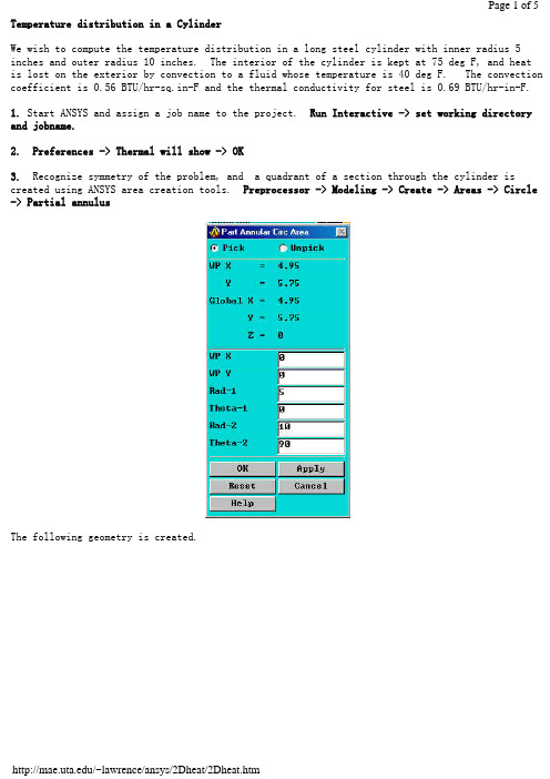
Temperature distribution in a CylinderWe wish to compute the temperature distribution in a long steel cylinder with inner radius 5 inches and outer radius 10 inches. The interior of the cylinder is kept at 75 deg F, and heatis lost on the exterior by convection to a fluid whose temperature is 40 deg F. The convection coefficient is 0.56 BTU/hr-sq.in-F and the thermal conductivity for steel is 0.69 BTU/hr-in-F.1. Start ANSYS and assign a job name to the project. Run Interactive -> set working directory and jobname.2. Preferences -> Thermal will show -> OK3. Recognize symmetry of the problem, and a quadrant of a section through the cylinder is created using ANSYS area creation tools. Preprocessor -> Modeling -> Create -> Areas -> Circle -> Partial annulusThe following geometry is created.4. Preprocessor -> Element Type -> Add/Edit/Delete -> Add -> Thermal Solid -> Solid 8 node 77 -> OK -> Close5. Preprocessor -> Material Props -> Isotropic -> Material Number 1 -> OKEX = 3.E7 (psi)DENS = 7.36E-4 (lb sec^2/in^4)ALPHAX = 6.5E-6PRXY = 0.3KXX = 0.69 (BTU/hr-in-F)6. Mesh the area and refine using methods discussed in previous examples.7. Preprocessor -> Loads -> Apply -> Temperatures -> NodesSelect the nodes on the interior and set the temperature to 75.8. Preprocessor -> Loads -> Apply -> Convection -> LinesSelect the lines defining the outer surface and set the convection coefficient to 0.56 and the fluid temp to 40.9. Preprocessor -> Loads -> Apply -> Heat Flux -> LinesTo account for symmetry, select the vertical and horizontal lines of symmetry and set the heat flux to zero.10. Solution -> Solve current LS11. General Postprocessor -> Plot Results -> Nodal Solution -> TemperaturesThe temperature on the interior is 75 F and on the outside wall it is found to be 45. These results can be checked using results from heat transfer theory.BackThermal Stress of a Cylinder using Axisymmetric ElementsA steel cylinder with inner radius 5 inches and outer radius 10 inches is 40 inches long and has spherical end caps. The interior of the cylinder is kept at 75 deg F, and heat is lost on the exterior by convection to a fluid whose temperature is 40 deg F. The convection coefficient is 0.56 BTU/hr-sq.in-F. Calculate the stresses in the cylinder caused by the temperature distribution.The problem is solved in two steps. First, the geometry is created, the preference set to'thermal', and the heat transfer problem is modeled and solved. The results of the heat transfer analysis are saved in a file 'jobname.RTH' (Results THermal analysis) when you issue a save jobname.db command.Next the heat transfer boundary conditions and loads are removed from the mesh, the preference is changed to 'structural', the element type is changed from 'thermal' to 'structural', and the temperatures saved in 'jobname.RTH' are recalled and applied as loads.1. Start ANSYS and assign a job name to the project. Run Interactive -> set working directory and jobname.2. Preferences -> Thermal will show -> OK3. A quadrant of a section through the cylinder is created using ANSYS area creation tools.4. Preprocessor -> Element Type -> Add/Edit/Delete -> Add -> Solid 8 node 77 -> OK ->Options -> K3 Axisymmetric -> OK5. Preprocessor -> Material Props -> Isotropic -> Material Number 1 -> OKEX = 3.E7 (psi)DENS = 7.36E-4 (lb sec^2/in^4)ALPHAX = 6.5E-6PRXY = 0.3KXX = 0.69 (BTU/hr-in-F)6. Mesh the area using methods discussed in previous examples.7. Preprocessor -> Loads -> Apply -> Temperatures -> NodesSelect the nodes on the interior and set the temperature to 75.8. Preprocessor -> Loads -> Apply -> Convection -> LinesSelect the lines defining the outer surface and set the coefficient to 0.56 and the fluid temp to 40.9. Preprocessor -> Loads -> Apply -> Heat Flux -> LinesSelect the vertical and horizontal lines of symmetry and set the heat flux to zero.10. Solution -> Solve current LS11. General Postprocessor -> Plot Results -> Nodal Solution -> TemperatureThe temperature on the interior is 75 F and on the outside wall it is found to be 43.12. File -> Save Jobname.db13. Preprocessor -> Loads -> Delete -> Delete All -> Delete All Opts.14. Preferences -> Structural will show, Thermal will NOT show.15. Preprocessor -> Element Type -> Switch Element Type -> OK (This changes the element to structural)16. Preprocessor -> Loads -> Apply -> Displacements -> Nodes(Fix nodes on vertical and horizontal lines of symmetry from crossing the lines of symmetry.)17. Preprocessor -> Loads -> Apply -> Temperature -> From Thermal AnalysisSelect Jobname.RTH (If it isn't present, look for the default 'file.RTH' in the root directory)18. Solution -> Solve Current LS19. General Postprocessor -> Plot Results -> Element Solution - von Mises StressThe von Mises stress is seen to be a maximum in the end cap on the interior of the cylinder and would govern a yield-based design decision.Back。
- 1、下载文档前请自行甄别文档内容的完整性,平台不提供额外的编辑、内容补充、找答案等附加服务。
- 2、"仅部分预览"的文档,不可在线预览部分如存在完整性等问题,可反馈申请退款(可完整预览的文档不适用该条件!)。
- 3、如文档侵犯您的权益,请联系客服反馈,我们会尽快为您处理(人工客服工作时间:9:00-18:30)。
实例1:某一潜水艇可以简化为一圆筒,它由三层组成,最外面一层为不锈钢,中间为玻纤隔热层,最里面为铝层,筒内为空气,筒外为海水,求内外壁面温度及温度分布。
几何参数:筒外径30 feet总壁厚 2 inch不锈钢层壁厚0.75 i nch玻纤层壁厚 1 inch铝层壁厚0.25 i nch筒长200 feet导热系数不锈钢8.27 B TU/hr.ft.o F玻纤0.028 BTU/hr.ft.o F铝117.4 BTU/hr.ft.o F边界条件空气温度70 o F海水温度44.5 o F空气对流系数 2.5 BTU/hr.ft2.o F海水对流系数80 BTU/hr.ft2.o F沿垂直于圆筒轴线作横截面,得到一圆环,取其中1度进行分析,如图示。
以下分别列出log文件和菜单文件。
/filename, Steady1/title, Steady-state thermal analysis of submarine/units, BFTRo=15 !外径(ft)Rss=15-(0.75/12) !不锈钢层内径ft)Rins=15-(1.75/12) !玻璃纤维层内径(ft)Ral=15-(2/12) !铝层内径(ft)Tair=70 !潜水艇内空气温度Tsea=44.5 !海水温度Kss=8.27 !不锈钢的导热系数(BTU/hr.ft.oF)Kins=0.028 !玻璃纤维的导热系数(BTU/hr.ft.oF) Kal=117.4 !铝的导热系数(BTU/hr.ft.oF)Hair=2.5 !空气的对流系数(BTU/hr.ft2.oF)Hsea=80 !海水的对流系数(BTU/hr.ft2.oF)/prep7et,1,plane55 !定义二维热单元mp,kxx,1,Kss !设定不锈钢的导热系数mp,kxx,2,Kins !设定玻璃纤维的导热系数mp,kxx,3,Kal !设定铝的导热系数pcirc,Ro,Rss,-0.5,0.5 !创建几何模型pcirc,Rss,Rins,-0.5,0.5pcirc,Rins,Ral,-0.5,0.5aglue,allnumcmp,arealesize,1,,,16 !设定划分网格密度lesize,4,,,4lesize,14,,,5lesize,16,,,2eshape,2 !设定为映射网格划分mat,1amesh,1mat,2amesh,2mat,3amesh,3/SOLUSFL,11,CONV,HAIR,,TAIR !施加空气对流边界SFL,1,CONV,HSEA,,TSEA !施加海水对流边界SOLVE/POST1PLNSOL !输出温度彩色云图finish菜单操作:1.U tility Menu>File>change jobename, 输入Steady1;2.U tility Menu>File>change title,输入Steady-state thermal analysis of submarine;3.在命令行输入:/units, BFT;4.M ain Menu: Preprocessor;5.M ain Menu: Preprocessor>Element Type>Add/Edit/Delete,选择PLANE55;6.M ain Menu: Preprocessor>Material Prop>-Constant-Isotropic,默认材料编号为1,在KXX框中输入8.27,选择APPL Y,输入材料编号为2,在KXX框中输入0.028,选择APPL Y,输入材料编号为3,在KXX框中输入117.4;7.M ain Menu: Preprocessor>-Modeling->Create>-Areas-Circle>By Dimensions ,在RAD1中输入15,在RAD2中输入15-(.75/12),在THERA1中输入-0.5,在THERA2中输入0.5,选择APPL Y,在RAD1中输入15-(.75/12),在RAD2中输入15-(1.75/12),选择APPL Y,在RAD1中输入15-(1.75/12),在RAD2中输入15-2/12,选择OK;8.M ain Menu: Preprocessor>-Modeling->Operate>-Booleane->Glue>Area,选择PICK ALL;9.M ain Menu: Preprocessor>-Meshing-Size Contrls>-Lines-Picked Lines,选择不锈钢层短边,在NDIV框中输入4,选择APPL Y,选择玻璃纤维层的短边,在NDIV框中输入5,选择APPL Y,选择铝层的短边,在NDIV框中输入2,选择APPL Y,选择四个长边,在NDIV中输入16;10.Main Menu: Preprocessor>-Attributes-Define>Picked Area,选择不锈钢层,在MAT框中输入1,选择APPL Y,选择玻璃纤维层,在MA T框中输入2,选择APPL Y,选择铝层,在MAT框中输入3,选择OK;11.Main Menu: Preprocessor>-Meshing-Mesh>-Areas-Mapped>3 or 4 sided,选择PICK ALL;12.Main Menu: Solution>-Loads-Apply>-Thermal-Convection>On lines,选择不锈钢外壁,在V ALI框中输入80,在V AL2I框中输入44.5,选择APPL Y,选择铝层内壁,在V ALI框中输入2.5,在V AL2I框中输入70,选择OK;13.Main Menu: Solution>-Solve-Current LS;14.Main Menu: General Postproc>Plot Results>-Contour Plot-Nodal Solu,选择Temperature。
对流换热系数定义:流体与固体表面之间的换热能力,比如说,物体表面与附近空气温差1℃,单位时间单位面积上通过对流与附近空气交换的热量。
单位为W/(m^2·℃)。
表面对流换热系数的数值与换热过程中流体的物理性质、换热表面的形状、部位、表面与流体之间的温差以及流体的流速等都有密切关系。
物体表面附近的流体的流速愈大,其表面对流换热系数也愈大。
如人处在风速较大的环境中,由于皮肤表面的对流换热系数较大,其散热(或吸热)量也较大。
对流换热系数可用经验公式计算,通常用巴兹公式计算。
的大致量级:空气自然对流 5 ~25 ,气体强制对流 20 ~100。
实例2:一钢铸件及其砂模的横截面尺寸如图所示:铸钢的热物理性能如下表所示:初始条件:铸钢的温度为2875o F,砂模的温度为80o F;砂模外边界的对流边界条件:对流系数0.014Btu/hr.in2.o F,空气温度80o F;求3个小时后铸钢及砂模的温度分布。
/Title, Casting Solidification!进入前处理/prep7et,1,plane55 !定义单元mp,dens,1,0.254 !定义砂模热性能mp,kxx,1,0.025mp,c,1,0.28mptemp,1,0,2643,2750,2875 !定义铸钢的热性能mpdata,kxx,2,1.44,1.54,1.22,1.22mpdata,enth,2,0,128.1,163.8,174.2mpplot,kxx,2mpplot,enth,2save!创建几何模型k,1,0,0,0k,2,22,0,0k,3,10,12,0k,4,0,12,0/pnum,kp,1/pnum,line,1/pnum,area,1/Triad,ltopkplota,1,2,3,4saverectng,4,22,4,8aplotaovlap,alladele,3aplotsave!划分网格esize,1amesh,5mat,2aplotamesh,4eplot/pnum,elem/number,1save!进入加载求解/SOLUantype,trans !设定为瞬态分析esel,s,mat,,2 !设定铸钢的初始温度nsle,s/replotic,all,temp,2875esel,inve !设定砂模的初始温度nsle,s/replotic,all,temp,80allselsavelplotsfl,1,CONV,0.014,,80 !设定砂模外边界对流sfl,3,CONV,0.014,,80sfl,4,CONV,0.014,,80/psf,conv,2time,3 !设定瞬态分析时间kbc,1 !设定为阶越的载荷autots,on !打开自动时间步长deltim,0.01,0.001,0.25 !设定时间步长timint,on !打开时间积分tintp,,,,1 !将THETA设定为1 outres,all,all !输入每个子步的结果solve!进入后处理/post26/pnum,node,1/number,0eplotnsol,2,204,temp,center !设定铸钢中心点温度随时间的变量plvar,2 !绘制温度~时间曲线savefinish菜单操作:1.Utility Menu>File>Change Title, 输入Casting Solidification;2.定义单元类型:Main Menu>Preprocessor>Element Type>Add/Edit/Delete, Add, Quad 4node55;3.定义砂模热性能:Main Menu>Preprocessor>Material Props>Isotropic, 默认材料编号1, 在Density(DENS)框中输入0.054, 在Thermal conductivity (KXX)框中输入0.025, 在Specific heat(C)框中输入0.28;4.定义铸钢热性能温度表:Main Menu>Preprocessor>Material Props>-Temp Dependent->TempTable, 输入T1=0,T2=2643, T3=2750, T4=2875;5.定义铸钢热性能:Main Menu>Preprocessor>Material Props>-Temp Dependent ->Prop Table,选择Th Conductivity,选择KXX, 输入材料编号2,输入C1=1.44, C2=1.54, C3=1.22, C4=1.22,选择Apply, 选择Enthalpy,输入C1=0, C2=128.1, C3=163.8, C4=174.2;6.创建关键点:Main Menu>Preprocessor>-Modeling->Create>Keypoints>In Active CS,输入关键点编号1,输入坐标0,0,0, 输入关键点编号2, 输入坐标22,0,0, 输入关键点编号3, 输入坐标10,12,0, 输入关键点编号4, 输入坐标0,12,0;7.创建几何模型:Main Menu>Preprocessor>-Modeling->Create>-Areas->Arbitrary>ThroughKPs,顺序选取关键点1,2,3,4;8.Main Menu>Preprocessor>-Modeling->Create>-Areas->Rectangle>By Dimension,输入X1=4,X2=22,Y1=4,Y2=8;9.进行布尔操作:MainMenu>Preprocessor>-Modeling->Operate>-Booleans->Overlap>Area,Pick all;10.删除多余面:Main Menu>Preprocessor>-Modeling->Delete>Area and Below,311.保存数据库:在Ansys Toolbar中选取SA VE_DB;12.定义单元大小:Main Menu>Preprocessor>-Meshing->Size Cntrls>-Global->Size, 在Element edge length框中输入1;13.对砂模划分网格:Main Menu>Preprocessor>-Meshing->Mesh>-Areas->Free,选择砂模;14.对铸钢划分网格:Main Menu>Preprocessor>-Attributes->Define>Default Attribs, 在Material number菜单中选择2;15.Main Menu>Preprocessor>-Meshing->Mesh>-Areas->Free,选择铸钢;16.定义分析类型:Main Menu>Solution>-Analysis Type->New Analysis, 选择Transient;17.选择铸钢上的节点:Utility Menu>Select>Entities, 选择element,mat,输入2,选择Apply,选择node, attached to element,选择OK;18.定义铸钢的初始温度:Main Menu>Solution>-Loads->Apply>Initial Condit’n>Define, 选择Pick all,选择temp, 输入2875, OK;19.选择砂模上的节点:Utility Menu>Select>Entities,Nodes, inverse20.定义砂模的初始温度:Main Menu>Solution>-Loads->Apply>Initial Condit’n>Define, 选择Pick all, 选择temp, 输入80, OK;21.Utility Menu>Select>Everything;22.Utility Menu>Plot>Lines;23.定义对流边界条件:Main Menu>Solution>-Loads->Apply>-Thermal->Converction>OnLines,选择砂模的三个边界1,3,4, 在file coefficent框中输入80, 在Bulk temperature框中输入, 80;24.设定瞬态分析时间选项:Main Menu>Solution>Load Step Opts>Time/Frequenc>Time-Time Step,Time at end of load step 3Time Step size 0.01Stepped or ramped b.c. SteppedAutomatic time stepping onMinimun time Step size 0.001Maximum time step size 0.2525.设置输出:Main Menu>Solution>Load Step Opts>Output Ctrls>DB/Results File, 在Filewrite frequency框中选择Every substep;26.求解:Main Menu>Solution>-Solve->Current LS;27.进入后处理: Main Menu>Timehist Postproc;28.定义铸钢中心节点的温度变量:Main Menu>Timehist Postproc>Define Variables, Add,Nodal DOF result,2,204;29.绘制节点温度随时间变化曲线:Main Menu>Timehist Postproc>Graph Variable,2。