ESA矢量分析软件操作手册
ESA数控折弯系统S540550中文操作手册v
1.3.1 要绘制的上模 ................................................................................................... 1.9
1.3.2 预设上模
...................................................................................................1.14
1.4如何输入一个新的上模 .....................................................................................................1.15 1.4.1 要绘制的下模............................. ........................................................................1.17 1.4.2 预设下模 ..........................................................................................................1.24
2.11.2 如何使用校正系数 ................................ .........................................................2.35
2.12 半自动模式校正 ................................ ..........................................................................2.36
ESA测温仪操作教程资料

3
4
3. Power(电源)指示灯:
测温仪连接电脑后,此指示灯点亮,红色灯 表示充电中,绿色表示充电完成。
2 6
4. Data(数据)指示灯:
测温仪中的数据状态指示灯。亮红灯表示存在数据;亮绿灯表示测试数据中。
5. Status(状态)指示灯:
测温仪的状态指示灯。熄灭时,表示测温仪在休眠状态,长亮绿灯表示待机状态。
测温仪资料下载流程
常规下载模式
测温仪资料下载流程图标,确定与该笔测试数据相关的产品资讯,客户及 炉子特性及设定资讯,可以方便的将曲线按客户、产品、生产线及工艺配 方进行分类管理及设定,具体如何设定或填写以上资料资讯。
对新建分类 需7步可下载
对已存在分类 需4步便可 下载
Reflow Process Won't Be Unsearchable Any More
五. 使用USB数据线连接测温仪至电脑;
出炉仪器温度较高,请 注意高温烫伤
停止数据记录
六. 打开Esamber Profiler测温仪软体, 在顶部工具栏内点击 “下载数据图 标,进行下载。
下载流程图标
具体下载流程请参考软件操作说明 Reflow Process Won't Be Unsearchable Any More
常规下载模式扩展
测温完毕,仪器冷却好后接USB连至电脑进行数据下载。
在功能选择区点击 ‘下载数据’项进 行下载。 新产品需填写3、4、 5、6项。 填写‘选择/建立工 艺规格’项可选择 历史‘参考规格’。 下载前要准备好产 品质料、锡膏资料、 工艺规格、焊炉资 料。
Reflow Process Won't Be Unsearchable Any More
ArcGIS 9.3 矢量数据分析工具使用说明书

Exercise 2: Working with Vector Data in ArcGIS 9.3Step1: Start ArcMap with a new project. Add the following data layers located in c:\REM402\idaho_utmData Layer Description Source Scale Boundary Idaho boundary Inside IdahoCounty Counties of Idaho Inside Idaho Road_100 Highways, roads and trails USGS 1:100,000 Stream_100 Streams USGS 1:100,000 idstwrd_utm Idaho ownership GAP data 1:100,000We will use this base data to create a GIS dataset for the Craig Mountain WildlifeManagement Area located south of Lewiston, Idaho north of the confluence of the Snake and Salmon River.Step 2: Add the Craig Mountain boundary to ArcMap. The boundary is a shape file located in the folder c:\REM402\Craig and named craig_bnd.shpClipCLIP operation: Clip one layer based on another. The CLIP operation works like acookie-cutter. In this exercise we will clip streams, roads and ownership to the boundary of Craig Mountain.Step 5: Use the Clip function to clip out streams (stream_100) and then ownership (idstwrd_utm) using the Craig Mountain boundary as the clip-layer.After you have created the subset layers of roads, streams and ownership you can remove the statewide layers from the project by right-clicking on the layer and select remove. This removes the layer from the map project, however the data file still resides in c:\REM402\Idaho_utm on your computer.Remember to save your work periodically!Xtools extensionXtools is a ‘third party’ extension (not created by ESRI) that can be downloaded at no cost from ESRI(/). Xtools is already on the GIS lab computers. Search on Xtools.After the search is done, select to download Xtools Pro 3.0.The downloaded file is compressed (zip) and must be uncompressed using the WinZip software. You can download WinZip for free from (search on WinZip) if you don’t have this software on your computer.Install the Xtools Pro 3.0 software on your computer.Create a summary table in ArcMapStep 6: Open the theme table for the ownership layer for the Craig Mountain ownership layer. Make sure the area has been updated according to above instructions. The attribute OWNERNAME designates the land-managing entity (BLM, Forest Service, Private etc.) for each one of the over 200 polygons in the table. In the next step you will create a summary table that summarizes the area for each owner category.IntersectThe INTERSECT operation is an overlay analysis between two vector data layers that creates an output data layer that contains the spatial and attribute information from both the input layers.For example, if we intersect the Craig Mountain ownership layer with the Idaho counties we create a layer that contains both the information about ownership and what county each polygon belongs to.Step 8: Use the ArcToolbox Analysis Tools to intersect the Craig Mountain ownership layer with the Idaho counties. Select Analysis Tools – Overlay – Intersect in ArcToolbox.Step 10: Notice how the arcs from the county layer have been incorporated into the ownership layer. The polygons along the county boundary have been split in two – one that resides in Lewis County and one that resides in Nez Perce County.The attribute table for the resulting theme contains information about both ownership and what county each polygon resides in.Proximity AnalysisIn natural resource applications proximity analysis (buffering) is often used to estimate area of riparian zone and habitat along streams. Roads, shorelines and legal boundaries are other features commonly buffered.Point locations can also be buffered. In analyses of wildlife habitat it is often of interest to determine what habitats are within a certain distance of animal observation locations such as nests, foraging areas, etc.In the following exercise you will buffer the streams on Craig Mountain and calculate how much area is within 30 m of a stream.Step 12: Select Analysis Tools – Proximity – Buffer in ArcToolbox. Buffer the streams on Craig Mountain with a 30 m buffer (make sure to buffer the streams on Craig Mountain rather than all of the streams in Idaho!!).Step 13: Use Xtools to update the area for the stream buffer. How much area on Craig Mountain is within 30 m of a stream?Save the project. You will be using this project in the next lesson!Deliverables Lesson 21. A map displaying the land owner categories on Craig Mountain. Also include roads and streams on the map. Include a legible legend, scalebar, northarrow etc.2. The summary table of area in different land ownership created as part of this lab.3. An estimate for how much area is within 30 meters of a stream on Craig Mountain. Please compile all deliverables in ONE document before submitting in Blackboard!。
ESPS用户操作手册
ESPS用户操作手册目录一、键盘介绍 (2)二、主菜单屏幕选项简介 (2)三、帮助菜单具体介绍 (3)四、操作菜单功能具体介绍 (8)4.1编辑运行范围 (8)4.2报警极限设置 (14)4.3反电晕工作方式 (16)4.4脉冲供电方式 (19)4.5变压器/整流器额定设置 (21)4.6微火花响应模式 (25)4.7密码设置 (26)五、操作屏幕状态显示 (27)5.1主状态显示 (27)5.2一次电流、电压和SCR 控制角 (30)5.3二次电流、电压 (31)5.4二次电流的衰减 (32)5.5波形分析显示 (32)5.6观察模拟输入和6 分钟的平均功率KW (33)5.7被测主线频率 (33)一、键盘介绍数字键——<0-9>数字键用以输入数据和选择菜单功能。
(0和1键为双重功能键)上、下箭头键——用来屏幕显示翻页左、右箭头键——输入数据时打空格键——用来存储数据或者锁存显示键——此键将回复到菜单设置状态1/RUN键——此键为绿色。
在输入数据时,它为数值1;在正常的ESP-S1操作中,当操作屏幕显示时,此键将启动ESP-S1的运行。
如ESP-S1已经处在工作状态,此键将重新启动斜率搜索。
HALT键——此键为红色。
在输入数据时,它为数值0;在正常ESP-S1操作中,当操作屏幕显示时,按下此键将会使火花消失,从而使ESP-S1操作停止,如ESP-S1已经处于报警停滞状态,按此键可消除报警。
键——在输入数据时,此键用来储存输入的数据和设置。
在正常ESP-S1操作中,按此键将锁存主要状态显示《DISPLAY HOLD》30秒钟,以便于操作人员记录读数。
运行中按此键将不会影响控制系统的工作。
二、主菜单屏幕选项简介ESP-S1共有三个主菜单屏幕,操作人员可以获取所有的控制功能和帮助菜单。
在主菜单显示的情况下,按下相应的数字键即可进入不同的操作。
我们先对每个操作选项加以简单的介绍。
系统通电后在键盘按下键,即可从主菜单进入第一主菜单(ESP-S1 Main Menu 1),此菜单具体选项如下:1、帮助菜单(Help Menu)——进入帮助菜单显示,这里可以帮助您解决在实际操作应用中遇到的个中问题。
Agilent ESA-L Series 电磁波分析器数据手册说明书
AgilentESA-L Series Spectrum AnalyzersData SheetAvailable frequency rangesE4411B 9 kHz to 1.5 GHzE4403B 9 kHz to 3.0 GHzE4408B 9 kHz to 26.5 GHzAs the lowest cost ESA option, these basic analyzersare ideal for cost conscious bench-top or manufacturingenvironments.Customers looking for a more portable solution wouldbenefit from the new Agilent N9340B handheld RFspectrum analyzer.Customers looking for a lower cost alternative to theESA-L should consider the Agilent N9320B handheldRF spectrum analyzer.1981The ESA-L Series spectrum analyzers are tested to ensure they will meet their warranted performance. Unless otherwise stated, all specifications are valid over 0 to55 °C. Supplemental characteristics, shown in italics, are intended to provide additional information that is useful in using the instrument. These typical (expected) or nominal performance parameters are not warranted but represent performance that 80 percent of the units tested exhibit with 95 percent confidence at room temperature (20 to 30 °C). This data sheet is intended as a quick reference to ESA-L spectrum analyzer specifications, and is by no means complete. Please refer to the ESA-L specification guide for full information and specifications, publication number: E4403-90036.Table of ContentsDefinition of Specifications (2)ESA-L Express Analyzer Option BAS or BTG (3)Frequency Specifications (4)Amplitude Specifications (7)Tracking Generator Specifications (12)General Specifications (13)23Receive faster delivery and a favorable price when you order the ESA-L express analyzer Option BAS or BTG. This express analyzer is confi gured based on the most frequently ordered ESA-L confi guration and most popular options. The express analyzer options simplify the ordering process while maintaining the fl exibility of the ESA platform.Customers looking for a more portable solution would benefi t from the new handheld spectrum analyzer N9340B./fi nd/N9340BCustomers looking for a lower cost alternative to the ESA should consider the /fi nd/N9320BChoose your frequency range:E4411B9 kHz to 1.5 GHz E4403B 9 kHz to 3.0 GHz E4408B9 kHz to 26.5 GHzChoose your express option:BAS Includes IF/sweep port (A4J) and GPIB connection (A4H)BTG Includes BAS, plus tracking generator functionalityAnd receive the following advantages:• 1.1 dB overall amplitude accuracy • +7.5 dBm TOI• 1 kHz minimum RBW•100 Hz minimum RBW with Option 1DNThe BAS or BTG express option can be combined with Option 1DN, narrow resolution bandwidth.ESA-L Express Analyzer Option BAS or BTGFrequency Specifications6Offset from CW signal ≥ 10 kHz –93, –95 dBc/Hz –100, –105 dBc/Hz –106, –112 dBc/Hz –118, –122 dBc/Hz –100, –102 dBc/Hz –104, –106 dBc/Hz –113, –116 dBc/Hz–90, –94 dBc/Hz ≥ 20 kHz ≥ 30 kHz ≥ 100 kHzResidual FM (peak-to-peak)StabilityNoise sidebands offset from CW signal with 1 kHz RBW, 30 Hz VBW and sample detector Specification and typical dBc/Hz applies to all frequencies ≤ 6.7 GHz a, bItalics indicate typical performance ≥ 30 kHz offset from carrier CW signalSystem related sidebands≤ –65 dBc + 20logN b 1 kHz RBW,1 kHz VBW (measurement time)≤ 150 Hz x N b (100 ms)≤ 30 Hz x N b (20 ms), Option 1DRE4411BE4403B/08Ba. Add 20log(N) for frequencies > 6.7 GHz.b. N = LO harmonic mixing number.Frequency Specifications (continued)E4411B E4403B E4408B Frequency1 - 10 MHz10 - 500 MHz500 MHz - 1 GHz1 - 1.5 GHz1.5 - 2 GHz2 -3 GHz3 - 6 GHz 6 - 12 GHz 12 - 22 GHz N/AN/A22 - 26.5 GHz –123, –129–123, –130–124, –129–127, –131–125, –130–125, –130–124, –130–122, –130–121, –128–120, –128–118, –127–115, –124–109, –122–126–129Displayed average noise level (dBm) (input terminated, 0 dB attenuation, sample detector) specificationItalics indicate typical performanceConditions100 Hz RBW; 1 Hz VBW (Option 1DR);810Tracking Generator SpecificationsFrequency rangeE4411BOption 1DN, (50 Ω) 9 kHz to 1.5 GHzOption 1DQ, (75 Ω ) 1 MHz to 1.5 GHzRBW range 1 kHz to 5 MHzOutput power level rangeE4411BOption 1DN 0 to –70 dBmOption 1DQ +42.75 to –27.25 dBmVOutput vernier rangeE4411B 10 dBOutput attenuator rangeE4411B 0 to 60 dB, 10 dB stepsOutput flatnessE4411BOption 1DN, (50 W)9 kHz to 10 MHz ±2.0 dB10 MHz to 1.5 GHz ±1.5 dBOption 1DQ, (75 W)1 to 10 MHz ±2.5 dB10 MHz to 1.5 GHz ±2.0 dBEffective source match (characteristic)E4411B < 2.5:1Spurious outputHarmonic spursE4411B(0 dBm output)9 kHz to 20 MHz < –20 dBc20 MHz to 1.5 GHz < –25 dBcNon-Harmonic spursE4411B < –35 dBcDynamic range Maximum output power – displayed average noise level Output power sweep rangeE4411BOption 1DN (–15 to 0 dBm) - (source attenuator setting)Option 1DQ (+27.75 to +42.75 dBmV) - (source attenuator setting) 1214Front panel Input 50 Ω type N (f); 75 Ω BNC (f) (Option 1DP); 50 Ω APC 3.5 (m) (Option BAB) RF out50 Ω type N (f); 75 Ω BNC (f) (Option 1DQ)Probe power +15 Vdc, –12.6 Vdc at 150 mA maximum (characteristic)External keyboard 6-pin mini-DIN, PC keyboards (for entering screen titles and file names) Headphone Front panel knob controls volume Power output0.2 W into 4 Ω (characteristic) AMPT REF out50 Ω BNC (f) (nominal) IF INPUT (Option AYZ)50 Ω SMA (f) (nominal) LO OUTPUT (Option AYZ)50 Ω SMA (f) (nominal)Rear panel10 MHz REF OUT 50 Ω BNC (f), > 0 dBm (characteristic)10 MHz REF IN50 Ω BNC (f), –15 to +10 dBm (characteristic) GATE TRIG/EXT TRIG IN BNC (f), 5 V TTL GATE /HI SWP OUT BNC (f), 5 V TTLVGA OUTPUTVGA compatible monitor, 15-pin mini D-SUB, (31.5 kHz horizontal, 60 Hz vertical sync rates, non-interlaced analog RGB 640 x 480)IF, sweep and video ports (Option A4J or AYX)AUX IF OUT BNC (f), 21.4 MHz, nominal –10 to –70 dBm (uncorrected) AUX VIDEO OUT BNC (f), 0 to 1 V, characteristic (uncorrected) HI SWP IN BNC (f), low stops sweep, (5 V TTL) HI SWP OUT BNC (f), (5 V TTL) SWP OUT BNC (f), 0 to +10 V ramp GPIB interface (Option A4H)IEEE-488 bus connector Serial interface (Option 1AX)RS-232, 9-pin D-SUB (m)Parallel interface (Option A4H or 1AX)25-pin D-SUB (f) printer port only Dimensions and weight for the ESA family of analyzers. Width to outside of instrument handle 416 mm (16.4 in) Width to outside of the shipping cover 373 mm (14.7 in) Overall height222 mm (8.75 in) Depth from front frame to rear frame409 mm (16.1 in) Depth with instrument handle rotated horizontal 516 mm (20.3 in)E4411BInstrument weight 13.2 kg (29.1 lbs) Shipping weight 25.1 kg (55.4 lbs) E4403BInstrument weight 15.5 kg (34.2 lbs) Shipping weight 27.4 kg (60.4 lbs) E4408BInstrument weight 17.1 kg (37.7 lbs) Shipping weight 31.9 kg (70.3 lbs)I/O connectivity software IO libraries suite (/find/iosuite/data-sheet )General Specifications (continued)For More InformationFor the latest information on the Agilent ESA-L Series see our Web page at:/find/esa/fi nd/emailupdatesGet the latest information on theproducts and applications you select./fi nd/agilentdirectQuickly choose and use your testequipment solutions with confi dence.Agilent Email UpdatesAgilent DirectRemove all doubtOur repair and calibration services will get your equipment back to you, performing like new, when prom-ised. You will get full value out of your Agilent equipment through-out its lifetime. Your equipment will be serviced by Agilent-trained technicians using the latest factory calibration procedures, automated repair diagnostics and genuine parts. You will always have the utmost confi dence in your measurements. Agilent offers a wide range of ad-ditional expert test and measure-ment services for your equipment, including initial start-up assistance, onsite education and training, as well as design, system integration, and project management.For more information on repair andcalibration services, go to:/fi nd/open Agilent Open simplifi es the process of connecting and programming test systems to help engineers design, validate and manufacture electronic products. Agilent offers open connectivity for a broad range of system-ready instruments, open industry software, PC-standard I/O and global support, which are combined to more easily integrate test system development.Agilent Open/fi nd/removealldoubt/find/esaFor more information on Agilent T echnologies’ products, applications or services, please contact your local Agilent office. The complete list is available at:/fi nd/contactusAmericasCanada (877) 894-4414 Latin America 305 269 7500United States (800) 829-4444Asia Pacifi c Australia 1 800 629 485China 800 810 0189Hong Kong 800 938 693India 1 800 112 929Japan 0120 (421) 345Korea 080 769 0800Malaysia 1 800 888 848Singapore 180****8100Taiwan 0800 047 866Thailand 1 800 226 008 Europe & Middle EastAustria 01 36027 71571Belgium 32 (0) 2 404 93 40 Denmark 45 70 13 15 15Finland 358 (0) 10 855 2100France 0825 010 700* *0.125 €/minute Germany 07031 464 6333****0.14 €/minuteIreland 1890 924 204Israel 972-3-9288-504/544Italy 39 02 92 60 8484Netherlands 31 (0) 20 547 2111Spain 34 (91) 631 3300Sweden 0200-88 22 55Switzerland 0800 80 53 53United Kingdom 44 (0) 118 9276201Other European Countries: /fi nd/contactusRevised: July 17, 2008Product specifi cations and descriptions in this document subject to change without notice.© Agilent Technologies, Inc. 2008Printed in USA, September 12, 20085989-9556EN。
Agilent_频谱分析仪使用手册.

f
2f
3f
非线性引起失真信号变化规律
失真信号/输入功率比(dBc)
失真信号幅度与混频器工作电平的关系
0
.
-20
二二阶阶
-40
-60
-80
三三阶阶
-100
-60
-30
混频器工作电平
0 TOI SHI +30
混频器工作电平 = 输入信号电平 - 衰减器设值
为减小频谱分析仪内部失真,混频器应工作在尽量低电平,应加大衰减器设值
=
相位误差
I
(average error magnitude) x 100%
(maximum symbol magnitude)
调制信号精度分析过程
解调
被测信号
标准参考信号 001110
调制器
误差信号
调制信号精度测试
ESA的数字调制信号分析能力
ESA-E Series Spectrum Analyzer
频谱分析仪性能指标 ------内部失真
< -50 dBc
< -40 dBc
< -50 dBc
三阶交调测试
各次谐波测试
频谱分析仪典型测试应用
频谱分析仪产生内部失真的原因
混频器非线性作用
混频信号
被测信号
混频器输出信号
混频器产生失真成分
各阶非线性失真变化规律
高阶失真信号幅度比基波信号变化速度快
3
Power in dB
频谱仪噪声会影响被测信号功率测试
Apparent Signal
Actual S/N
Displayed
S/N 频谱仪显示信号=输入信号+内部噪声
arcgis矢量化基本操作全解
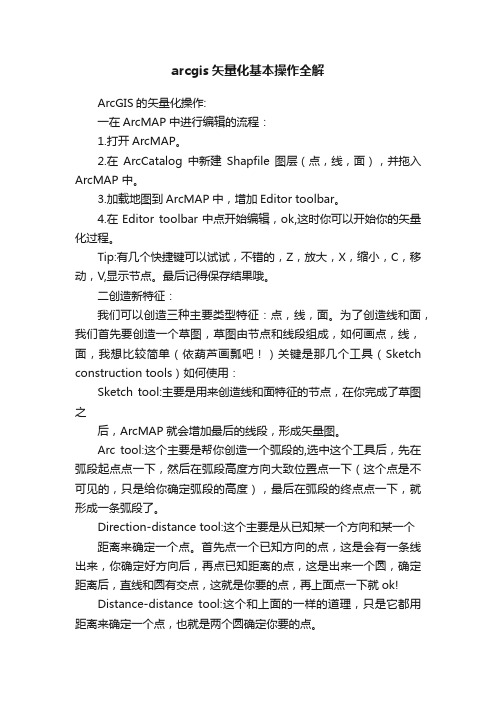
arcgis矢量化基本操作全解ArcGIS的矢量化操作:一在ArcMAP中进行编辑的流程:1.打开ArcMAP。
2.在ArcCatalog中新建Shapfile图层(点,线,面),并拖入ArcMAP 中。
3.加载地图到ArcMAP中,增加Editor toolbar。
4.在Editor toolbar中点开始编辑,ok,这时你可以开始你的矢量化过程。
Tip:有几个快捷键可以试试,不错的,Z,放大,X,缩小,C,移动,V,显示节点。
最后记得保存结果哦。
二创造新特征:我们可以创造三种主要类型特征:点,线,面。
为了创造线和面,我们首先要创造一个草图,草图由节点和线段组成,如何画点,线,面,我想比较简单(依葫芦画瓢吧!)关键是那几个工具(Sketch construction tools)如何使用:Sketch tool:主要是用来创造线和面特征的节点,在你完成了草图之后,ArcMAP就会增加最后的线段,形成矢量图。
Arc tool:这个主要是帮你创造一个弧段的,选中这个工具后,先在弧段起点点一下,然后在弧段高度方向大致位置点一下(这个点是不可见的,只是给你确定弧段的高度),最后在弧段的终点点一下,就形成一条弧段了。
Direction-distance tool:这个主要是从已知某一个方向和某一个距离来确定一个点。
首先点一个已知方向的点,这是会有一条线出来,你确定好方向后,再点已知距离的点,这是出来一个圆,确定距离后,直线和圆有交点,这就是你要的点,再上面点一下就ok!Distance-distance tool:这个和上面的一样的道理,只是它都用距离来确定一个点,也就是两个圆确定你要的点。
Endpoint arc tool:这也是创造弧段用的,与Arc tool 工具不同的是,它是先在弧段的起点点一下,然后在弧段的终点点一下,再点一个点确定弧段的半径。
个人认为这个工具要比Arc tool工具更精确些。
矢量网络分析仪使用步骤

2014-12-5
Vanchip Confidential
Confidential
示例矢量网络分析仪型号
示例用的仪器型号是Agilent E5071C ,该 仪器是双端口网分(9K~6.5GHz)。
(下文简称矢量网路分析仪为网分) 使用仪器示范: 第一步:校准仪器(包括固定线缆部分) 第二步:校准延长线 第三步:待测对象测量 第四步:阻抗匹配
1端口
2端口
Vanchip Confidential
Confidential
1端口延长线缆(同轴半硬线)
第1焊点, 就近焊接在待测位 置,就近接地(特别重要)!
硬线刚性较强,容易拉坏 PCB上的小焊盘,使用时 特别小心。
第2加固焊点, PCB板上加强焊接 ,避免1焊点在用力时拉掉焊盘。
Vanchip Confidential
Confidential
自动补偿的损耗值(延长线的实际损耗)
Vanchip Confidential
Confidential
延长线缆补偿状态SAVE
Vanchip Confidential
Confidential
第三步:待测对象测量
Vanchip Confidential
Confidential
Vanchip Confidential
Confidential
校准状态储存SAVE和Recall
按Save键,存储校准好的 状态。便于以后调用。
按Recall键,调用之前存 储好的校准状态。
Vanchip Confidential
Confidential
储存为自建文件---可长期使用
存储为自建文件名
- 1、下载文档前请自行甄别文档内容的完整性,平台不提供额外的编辑、内容补充、找答案等附加服务。
- 2、"仅部分预览"的文档,不可在线预览部分如存在完整性等问题,可反馈申请退款(可完整预览的文档不适用该条件!)。
- 3、如文档侵犯您的权益,请联系客服反馈,我们会尽快为您处理(人工客服工作时间:9:00-18:30)。
ESA-E4402B 矢量分析软件操作手册一、计算机、硬件的I/O连接及矢量分析软件安装本软件主要是利用ESA收集到的信号资源通过数字信息的方式与电脑之间进行传输,然后利用电脑的强大计算能力将收集的信号数字信息进行矢量分析及相关操作。
首先要安装I/O软件,放入相应光盘,点击“安装软件”即可自动进入安装程序,安装完毕后,桌面会出现“Agilent Connection Expert”,点击后即进入I/O接口软件界面:点击“USB/GPIB(GPIB0)”选项,即出现:表示硬件还没有连接上计算机,这是需要将ESA和计算机USB口的连接线拿出,在ESA处于关机状态时(连接线请勿热拔插),将ESA和计算机进行连接,连接线连接完成后,启动ESA,然后点击“”,即出现更新窗口,当更新完成后,图标前的小红叉即会变成绿色小钩,表示连接完成!下面介绍本矢量分析软件的安装:首先将相应的光盘放进光驱,出现安装界面后,点击“安装Agilent 89600 VSA”进入正式安装。
安装完成后会在桌面出现“Vector Signal Analyzer”“Spectrum Analyzer”两个图标。
点击第一个即可进入操作软件界面:二、功能按键详解软件操作分为11大项:FILE 、EDIT 、CONTROL 、SOURCE 、INPUT 、MEAS-SETUP 、DISPLAY 、TRACE 、MARKERS 、UTILITIES 、HELP。
①FILE其界面如下:Recall 调用Preset 重新设定Save保存数据,界面如下:Recall:Preset:Save:其中:三项菜单的前四项分别为:(调用/重设/保存)设置、(调用/重设/保存)菜单工具栏、(调用/重设/保存)颜色、字体等外观显示、(调用/重设/保存)光谱图的颜色显示。
State Definitions (State Defs…):规定精确度Recall Recording调出保存的信号图像Preset All将所有设置均重置,恢复原始设置。
Save Recording 保存信号图像。
Copy Trace 为拷贝正处于活动状态(ACTIVE)的某一信号轨迹Remove Register 清除数据寄存器的登陆、注册Print 、Print Setup 、Print Options 为常用打印菜单,打印正处于活动状态ACTIVE轨迹Exit 关闭矢量分析软件②EDIT其界面如下:Undo 取消最后一个已经应用的动作(后退)Copy Trace Data 将当前的轨迹数据写入剪切版Copy Text 将当前文字框里的内容写入剪切版Copy Markers 将当前标记点的数据写入剪切版③CONTROL 其界面如下:Restart 开始一项新测试活动Pause/Single. 暂停/单步执行某一测试Stop 停止当前的测试Disconnect 切断矢量分析软件和硬件之间的通讯联系Record 播放记录的信号Player 打开波形重放特写面板,界面如下:Sweep 切换间断扫描或者连续扫描④SOURCE其界面如下:⑤INPUT其界面如下:Channels 选择1或2输入通道(E4402B只有1个输入通道)Range 为输入信道设定输入范围Coupling 选择交流或直流耦合方式,其总界面如下:其中:Connection 线路种类Reference Impedance 参考阻抗值Trigger 选择触发信号的种类,其界面如下:Data From 选择输入信道信号或者记录的信号:Recording 设置记录参数,界面如下:(图中为记录时需要设置的参数)⑥MeasSetup其界面如下:Frequency Bands 选择合适的频带,有2种方式选择(一般我们选择36MHz-6GHz):Frequency 设置中心频率、带宽的方式;或者是起始频率的方式,界面如下:其中:Frequency step 频率步距Auto Frequency Step 为设置自动设定频率步距,为频带宽度的1/10。
Full Span 设置带宽为最大值From Spec Analyzer 设置矢量分析软件(Vector Signal Analyzer application)的频率参数与频谱分析软件(Spectrum Analyzer)软件相匹配Signal Track 选择根据输入信道的信号频率飘移而自动改变中心频率Time Data 选择在开始频率为0Hz的时候启动分析器的数字本机震荡器,默认为不启动。
(Zoom为启动;Baseband为关闭)Mirror Frequency 当需要的检测的信号为镜像时,可通过此设置将其还原。
ResBW 设定参考带宽及窗口参数,界面如下:其中:ResBW 设定参考带宽ResBW Mode 包含两种模式(1-3-10和arbitrary),1)1-3-10模式中ResBW 的数值只能设会1×10^或者3×10^的倍数;2)Arbitrary模式中ResBW的数值可以任意设置。
ResBW Couple 决定参考带宽与频带宽度如何结合(3种方式选择)1)Auto 当改变带宽时,在测量速度与频率参考之间自动找到平衡点2)Offset 当改变带宽时,保持参考带宽与带宽之间的固定比率3)Fixed 当改变带宽时,不改变参考带宽Window Type 观察并改变频谱测量中运用的窗口函数,界面如下1)Uniform 矩形窗函数2)Hanning 汉宁窗函数3)Gaussian Top 高斯窗函数(高度动态范围)4)Flat Top 平顶窗函数(快速傅立叶变换的默认函数)Frequency Points 频率扫描点数,默认值为801。
Time 设定时间及时间门控的参数其中:Main Time Length为主时间长度Auto Time Resolution 设置自动时间跟踪Average 设置平均参数,界面如下:Average Type 选择平均计算函数,有六种函数选择:1)RMS (Video) 减小各点之间的数量级差异,有利于对于底部白噪音的滤波。
2)RMS (Video) Exponential 同上者,额外运用了指数平均数的方法3)Time 作用于时域,显示于下阶段分组图表4)Time Exponential 同上者,额外运用了指数平均数的方法5)Continuous Peak-Hold 只记录每个点上数值最大的那个时刻的点Count 指定要执行平均的数目Repeat Average 只对线形平均类型有效,(完成平均后分析软件不会停止,依旧在继续执行) Fast Average 加速平均的速度Update Rate 更新速度Demodulator 控制并调节解调及检波的种类其中:Demod Off 关闭解调功能Analog Demodulator 相似解调器,设定后,显示窗口为:Analog Demod Properties:可以选择AM 、FM、PM三种调制方式(AM单位可以选择am 或者%)FM 、PM可以选择1)Auto Carrier Phase自动载波相位调整2)Auto Carrier Frequency自动载波频率调整★Digital Demodulator 数字解调器,设定后,显示窗口为:★Digital Demod Properties:★Format tab 格式栏其中Preset to Standard 指定标准的数字通讯系统,自动设置参数(注:测试数字电视信号,一般可以选用DVB64的方式)Format 选择格式:其中:1)D8 PSK 8进制周期相位键控2)BPSK 2进制周期相位键控3)DQPSK 微积分周期相位键控4)D8PSK 微分8周期相位键控5)DVB QAM 数字电视广播的QAM信号6)EDGE 基于GSM增强型数据率传输7)FSK 频率键控8)MSK 最小化键控9)Offset QPSK 偏移积分周期相位键控10)QAM 正交幅度调制11)QPSK 积分周期相位键控12)VSB 残余边带View State Definitions 显示规定格式的定义:Symbol Rate 符号率Result length 结果长度,决定显示符号的个数Points/Symbol 每个符号分多少点显示(point per symbol)Filter tab 选择解调信号滤波,界面如下:其中:Measurement Filter 测量滤波器,有如下选择:1)Rect Filter 矩形波滤波器2)Root Raised Cosine Filter 分布式滤波器3)Gaussian Filter 高斯滤波器(主要应用于MSK 和FSK 信号)4)User-defined Filters 用户自定义滤波器5)Low Pass Filter (for FSK) 低通滤波器6)IS-95 Base EQ 美国CDMA标准7)Raised Cosine Filter 升余弦滤波器Reference Filter 参考滤波器(选项解释同上)Data Register 数据寄存器Alpha/BT 设置耐奎斯特滤波器(Alpha)和高斯滤波器(BT)的滤波器特性英文介绍:Allowable values, non-Gaussian filters: .05 to 1Allowable values, Gaussian filters: .05 to 100Minimum increment: .01Increment using arrow keys or mouse wheel: .05 Search tab 设置脉冲查询或同步查询Pulse Search 脉冲查询Sync Search 同步查询Search Length 查询长度Search Offset 查询偏移量Search Pattern 查询图案Compensate tab 调节数字解调器的参数,界面如下:其中:Clock Adjust 时钟调节,决定数字解调器何时取样I/Q轨线。
最小值: -0.5 symbols最大值: +0.5 symbols Rotation 设置旋转角度IQ Normalize IQ规格化Mirror Frequency Spectrum (Digital Demodulation) 频谱镜像Equalization Filter 均衡滤波器Filter Length 滤波长度(3-99 symbols)Convergence 收敛度确定均衡滤波器的会聚程度Adaptive Equalization均衡适应化消除线性误差,并应用一个前馈修正滤波器(RUN 开始HOLD 停止)3G Cellular 3G信号调制,分四种:(介绍略)Wireless Networking 无线网络调制,分为(介绍略)Broadband Wireless Access 带宽无线通道调制:⑦DISPLAY 其界面如下:其中:Menu/Toolbars 定制显示菜单及工具栏的现显选项,其界面如下:Toolbars 制定工具栏及菜单的现示Tools 选择项目添加到菜单或工具栏里Options 设置软件里的全面显示选项Appearance 设置显示外观(颜色、字体、轨迹位置等)Layout 设置排版(显示窗口的排版)Active Trace 选择活动的窗口轨迹View/Overlay Traces 选择所要观察的窗口轨迹⑧TRACE 其界面如下:其中:Data选择测试结果的显示方式,界面如下:其中:Auto Correlation两个信号的相关性测量CCDF 互补积累分布函数CDF 积累分布函数Correction 补偿硬件和软件处理方面产生的误差Gate Time 时间门函数(当起用数字解调器或模拟解调器时无效)Inst Main Time 瞬间时域数据Inst Spec 瞬间频域数据Main Time 主体时间记录信号PDF 密度函数(数字解调时无效)PSD 功率谱密度函数Raw Main Time 未处理的硬件输入信号Spectrum 频谱信号Math 数学函数的结果显示Register 显示选择的数据存储器的内容Marker - ACPR 标记处的邻信道功率比Marker - OBW 标记处占有频率带宽Format 设定匹配Y轴,界面如下:其中:Format 界面如下:Log Mag(dB)对数显示形式Linear Mag 线形显示形式Real (I) 数字解调中显示I/Q波形中的I部分Imag (Q) 数字解调中显示I/Q波形中的Q部分Wrap Phase 限制相位显示(-180 到+180)Unwrap Phase 自由相位显示Group Delay 群延时显示I-Q (Digital Demodulation) IQ图表显示,(极矢量显示I显示于X轴Q显示于Y轴)Constellation (Digital Demodulation) 星座图(IQ图中符合符号时钟周期的点)Q-Eye (Digital Demodulation) Q眼图I-Eye (Digital Demodulation) I眼图Trellis-Eye (Digital Demodulation) 显示时间在X轴;显示展开相位在Y轴。