ansys workbench电磁场仿真完整例子
ansys workbench电磁场仿真完整例子
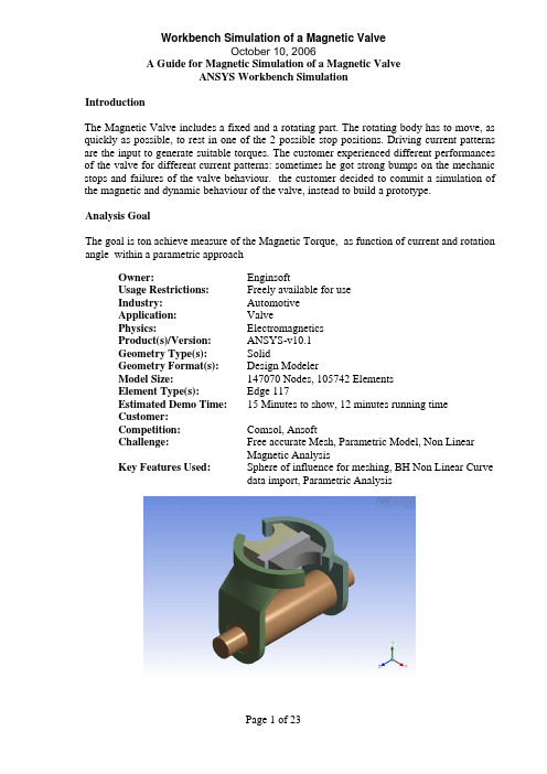
IntroductionThe Magnetic Valve includes a fixed and a rotating part. The rotating body has to move, as quickly as possible, to rest in one of the 2 possible stop positions. Driving current patterns are the input to generate suitable torques. The customer experienced different performances of the valve for different current patterns: sometimes he got strong bumps on the mechanic stops and failures of the valve behaviour. the customer decided to commit a simulation of the magnetic and dynamic behaviour of the valve, instead to build a prototype.Analysis GoalThe goal is ton achieve measure of the Magnetic Torque, as function of current and rotation angle within a parametric approachOwner:EnginsoftUsage Restrictions:Freely available for useIndustry:AutomotiveApplication:ValvePhysics:ElectromagneticsProduct(s)/Version:ANSYS-v10.1Geometry Type(s):SolidGeometry Format(s): Design ModelerModel Size:147070 Nodes, 105742 ElementsElement Type(s): Edge 117Estimated Demo Time:15 Minutes to show, 12 minutes running timeCustomer:Competition:Comsol,AnsoftChallenge:Free accurate Mesh, Parametric Model, Non LinearMagnetic AnalysisKey Features Used:Sphere of influence for meshing, BH Non Linear Curvedata import, Parametric AnalysisSteps and Points to Convey.Picture Guide.Start ANSYS Workbench Environment, and choose “New Geometry”.Importing of external geometrySet the desired length unit: meters.01) Click “File > Open > Import External Geometry File”.02) Click on “Generate” in order to confirm the importation of the geometry.The geometry regards a magnetic valve.Steps and Points to Convey.Picture Guide.Create a Parametric, Relative Rotation between two groups of bodies01) Create a local coordinate system (plane 4) by clicking on the “New Plane” icon in the tool bar.02) In “Details of Plane4 >. Type” choose from face in order to select the surface of interest. 03) Choose the space to the right of “Base Face” in Details of Plane4 and select the surface indicated in light blue in the plot at right.The local coordinate system “Plane 4” is now visible, centered on a face vertex04) In “Details of Plane4 >. Transform 1 (RMB)” insert an offset along X axis of –0.00825 m.05) In “Details of Plane4 >. Transform 1 (RMB)” insert an offset along Y axis of 0.0015 m.06) Click Generate to create Plane4Create another plane (Plane5).07) In “Details of Plane5 > Type” choose from plane. Base plane should be set to Plane4.08) In “Details of Plane5 >. Transform 1 (RMB)” insert a rotation about Z axis of 30°. 09) Click Generate to create Plane5.Steps and Points to Convey. Picture Guide.The local coordinate system “Plane 5” is now visible.10) From the tool bar menu, select “Tools > Freeze”.The freezing operation is indicated when bodies are displayed with transparency.11) From the tool bar menu, select “Create > Body Operation” set “Type” to “Move” click on the box to the right of Bodies.12) Select the bodies highlighted at right (use the Ctrl button to select multiple entities) and click Apply.Steps and Points to Convey.Picture Guide.13) In “Details of BodyOp1” choose the box to the right of “Source Plane” and pick on Plane4 in the Tree Outline.14) In a similar fashion, set “Destination Plane” to Plane5.Then click on “Generate” to move the parts as shown at right.ENCLOSURE definition01) From the tool bar menu, select “Tools >Enclosure” in order to insert a control volume cylindrically shaped and aligned to Y axis. Set the Cushion to 0.0375 m and set “Merge Parts?” to “Yes”.02) Click Generate to create the enclosureIn the “Outline” tree the just created enclosure is now visible.Steps and Points to Convey Picture GuideEnclosure is visible in the “Model View”window.CREATE the WINDING COIL01) In the Tree Outline, Open “1 Part, 7 Bodies > Part”. RMB on the last Solid in the list and choose “Hide Body” in the drop down menu. This will allow access to the surfaces of the imported geometry for forthcoming picking operations.02) Create a new plane (Plane6)03) In “Details of Plane6 >. Type” choose “From Face”.04) Click on the box to the right of “Base Face” and select the surface shown at right.05) In “Details of Plane6 >. Transform 1 (RMB)” insert an offset along Z axis of –0.0231 m.Click on Generate to create Plane6.06) With Plane6 now active, go to the tool bar and choose “New Sketch”.07) Select “Sketch1” in the “Tree Outline”.Steps and Points to Convey Picture Guide Sketching mode for winding coil generation08) Pick the Sketching tab at the bottom of theTree Outline09) Select “Circle” in the “Draw” window andchoose the center (origin of Plane6) and anarbitrary poin some distance away from thecenter to create a circle.10) Pick the Dimensions button at the bottom ofthe Sketching Toolboxes pane and choose“Radius”.11) Click on the circle and another arbitrarylocation for the radial dimension marker.12) In “Details of Sketch1”, modify the radiusR1 to be 0.00775 m.The sketch is now visible in the “Graphics”window.13) From the tool bar select “Concept > LineFrom Sketches”. Choose the circle and clickApply in the box to the right of “Base Objects”in “Details of Line1”. “Operation” should be setto “Add Material”.Click Generate.14) Choose the Line Body in the Tree Outline.15) In “Details of Line Body” set:•“Winding Body > Yes”•“Number of Turns” = 1•“CS Length” = 0.022 m•“CS Length” = 0.00375 mSteps and Points to ConveyPicture Guide16) From the tool bar, select “View > Show Cross Sections Solids”. The new winding body should appear as it does in the figure to the right.ANGLE as PARAMETER01) In the “Tree Outline” select “Plane5”02) Make the rotation about Z axis as parameter by clicking on the box to the left of “FD1, Value 1”.03) Rename the parameter as “angle”.Steps and Points to Convey.Picture Guide.04) From the tool bar, select “Tools > Options>Common Settings>Geometry Import”. Remove “DS” from the field to the right of “Personal Parameter Key” to remove the DS prefix naming convention restriction for importing parameters. Click OK.GO IN SIMULATIONIn the “[Project]” window, select “New Simulation”.In the “[Simulation]” window, the “Outline” tree should be as in figure.Steps and Points to ConveyPicture GuideMaterials Properties DefinitionSelect “Data” in the tool bar to open the “[Engineering Data]” window.Materials Properties Definitionchange defaults of STRUCTURAL STEEL01) Select “Structural Steel” and click on “Add/Remove Properties” in the “Electromagnetics” field and unselect the following items:- “Relative Permeability” - “Resistivity”02) Check the box to the left of “B-H curve” and click OK.03) Say “Yes” to the “Remove Material Properties” box that appears.04) Open excel file “bh1.xls” and copy the two data columns (highlight them with the mouse cursor and type Cntl-C).Steps and Points to ConveyPicture Guide05) Click the icon depicting an xy plot to the right of “B-H Curve”06) LMB on the 2 (second row) of the “Magnetic Flux Density vs. Magnetic Field Intensity” table and press “Ctrl +V” to paste the two column data from the .xls file.07) Click on the B-H Curve icon at the lower right.The curve should appear as shown at right.NEW Material definition IRONRMB on “Materials (2)” in the tree and choose “Insert New Material”. RMB on “New Material”, choose Rename and change the name of the new material to Iron. Define BH data as before but this time use data from “bh2.xls” file.NEW Material definition NEODYMIUM01) Define a New material named “Neodymium”.02) Among Electromagnetics properties let active just: “Linear Hard Material”: 03) Insert the following data:• Cohercive Force: 7.9577 e5 A/m • Residual Induction 1.2 T01) Return to the Simulation Tab02) In the Outline Tree, open Geometry>Part and use the Cntl button to select both of the RIC9512_105 items. The parts should be highlighted as shown at right.03) In Details of “Multiple Selection”, changematerial from “Structural Steel” to “Iron”Steps and Points to ConveyPicture Guide04) Select the part shown at right.05) Change material from “Structural Steel” to “Neodymium”MESH01) Select the coil support solid (see figure)02) RMB on “Mesh” on the tree to insert a sizing control: Element Size 2e-303) Insert another sizing control , 1e-3, referred to 5 bodies as in the following picture. It may help to hide the 4th solid (the “air enclosure) in the Outline tree to simplify selecting these parts.Steps and Points to ConveyPicture Guide5 bodies for sizing setting n.204) In the Outline tree, RMB on Model and insert a “Coordinate Systems” branch. RMB on the Coordinate Systems branch and insert (define) a new Coordinate System. Choose “Origin” in the Details of “Coordinate System” pane, select the surface shown at right, and click Apply.05) RMB on Mesh in the Outline to insert a third sizing control:For “Type”, choose “Sphere of Influence”• Sphere Center: Coordinate System (defined just before) • Radius 1.5e-2 • Element size 5e-4Areas to be applied are the following (10 areas)Steps and Points to ConveyPicture Guide10 Areas where to apply the Sphere of Influence sizing control06) Click on Mesh -> Preview MeshThe Mesh should result as in figure, if the “Air” solid enclosure body is hideLOADSSet the Conductor Current value in details window related to “Conductor Winding Body”: 1000 ABOUNDARY CONDITIONSRMB on Environment in the tree and insert a Magnetic Flux Parallel object. Use the Cntl button to select the 3 exterior surfaces of the enclosure and click Apply.Steps and Points to Convey.Picture Guide.POSTPROCESSING SETTINGS01) Insert under the “Solution” tree the following output requests: • Total Flux Density • Total Flux Intensity 02) Select 3 bodies as in figure03) Insert a “Directional Force/Torque” output request with details:• In Details of “Directional Force/Torque” pane, change “Global Coordinate System” to “Coordinate System” (this is the user-defined coordinate system centered on the top surface of the permanent magnet).• Set Orientation to Y Direction (rotation axis)04) repeat Directional Force/Torque Request for both X and Z axis direction05) By a right click under the Solution Tree Insert a “Solution Information” request to monitor the run during the solutionSOLVE01) Highlight the Environment tree tosee/check all Boundary & Loads previously defined.02) Click on the “SOLVE” Icon to launchthe run.Solution times takes about 12 minutes on a 2.8 Ghz single processor 32bit PCSteps and Points to ConveyPicture GuideREVIEW RESULTS01) See the Total Flux of Magnetic results 02) Set up a Vector Image of the MagneticField03) After Vector Image settings show a Vector Plot of Magnetic Field03)See the Magnetic Force distribution, Yaxis direction, on the requested parts. 04)The same for X, Z directions05)Activate the view from Y Global Axis06)Define a “Slice Plane”07)Draw the slice plane trace at nearlyalong the Y global direction08)View from the X Global direction09)Activate “show elements” and show themagnetic fieldSteps and Points to Convey Picture GuideSET UP A PARAMETRIC ANALYSIS01) Click on “Model”02) Click on CAD Parameters Detail toactivate the “angle” as a parameter. Thiswill be the first INPUT parameter.03) Click on Environment and Duplicate byright click04) Activate the Conductor Current Value asparameter. This is the second INPUTparameter n.2.05) Activate the Torque value in Y directionas OUTPUT parameter (ThirdParameter)06)Click on “Solution” of Environment 2and then click on Parameter Manager 07)Set up many cases as you like, forexample with 4 current values, 3 values other than the previously solved.。
ANSYS恒定磁场仿真演示

2个节点定 路径
后处理,设置显示路径
命名路径
往路径上映射变量的数值
准备显示路径上的变量,例如 磁感应强度的模
显示路径上变量的曲线
准备存储图形文件(抓图)
存储的图形文件
退出ANSYS软件界面
7、问题扩展
扩展的问题:
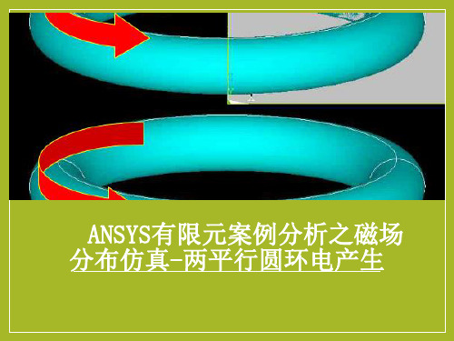
将电流通入4条圆柱形平行导线。 左侧两条电流向里,右侧两条电流向 外。计算这些电流产生的磁场。
Ansys 恒定磁场仿真演示
1、问题描述
问题:两平行圆环电流产生磁场分布仿真
求解区 域
6 1
3
问题:两平行圆环电流产生磁场分布仿真(轴对称模型)
2、软件启动
从”程序”开始,最后点 击“license status”
激活license,从“程序”开始。
点击server
点击server,激活。若不能激活,需等待所提示的时间
求解启动
点击 点击
提示信息 关闭求解信 息窗口
求解完毕
6、后处理
准备显示A的云图 (等位线)
后处理启动
后处理,显示矢量磁位云图
画磁感应强度 线
后处理,准备画磁感应强度线
后处理,画磁感应强度线(27条)
画矢量 箭头
准备显示磁感应强度矢量(箭头)
点击显示 控制菜单
放大 图形
放大后的磁感应强度矢量图
前处理,划分网格,选中内部区域
前处理菜单
选择三 角形, 自由网
格
划出 网格
5、求解
求解模块中的加载,选中小圆面积
加载,小圆面积上加电流密度激励
这两条边上加 边界条件
求解,加载,准备加第一类边界条件(A的边界值)
加边界条件(A=0)
选中无限单元 最外边界
ansys workbench建模仿真技术及实例详解 -回复
ansys workbench建模仿真技术及实例详解-回复什么是ANSYS Workbench建模仿真技术,以及提供一个实例来详解。
ANSYS Workbench建模仿真技术是一种集成在ANSYS软件平台下的先进仿真建模工具。
它能够提供全面的、高精度的仿真分析,用于解决各种工程问题。
ANSYS Workbench能够模拟并分析结构力学、流体动力学、热传导和电磁场等各种物理现象,它是一个功能强大且灵活的工具,可用于设计优化、性能评估和故障诊断等应用。
ANSYS Workbench的优势之一是其集成的工作环境。
它提供了一个统一的界面,允许工程师能够轻松地建立多物理场的模型、设置边界条件、进行网格划分以及执行仿真分析。
这个集成环境大大提高了工作效率,减少了因为转换格式而产生的错误和不一致性。
ANSYS Workbench还具有高度可扩展性。
它支持多种不同类型的分析,并且可以与其他工具和软件集成。
这使得工程师能够根据他们的特定需求,选择合适的分析方法和模型。
此外,ANSYS Workbench还可以通过添加插件和自定义脚本等方式进行扩展和定制化,以满足用户需求。
下面以一个实例来详细说明ANSYS Workbench建模仿真技术的应用。
假设我们要设计一个汽车的底盘,我们希望通过仿真分析来优化其刚度和强度。
首先,我们需要建立一个底盘的三维几何模型。
可以使用ANSYS SpaceClaim软件来创建几何模型,然后将其导入到ANSYS Workbench 中进行后续分析。
接下来,我们需要定义材料属性。
通过在材料库中选择合适的材料,并输入相应的力学参数,如弹性模量、泊松比和屈服强度等。
这些参数将用于定义底盘的材料行为。
然后,我们需要设定边界条件。
我们可以设定车轮的载荷、车身的支撑条件、底盘的连接方式等。
这些边界条件将用于约束和模拟底盘在实际工况下的受力情况。
接着,我们需要对几何模型进行网格划分。
ANSYS Workbench提供了多种网格划分工具,可以根据模型的复杂性和分析需求选择合适的网格类型和划分方法。
ANSYS有限元案例分析之磁场分布仿真案例
ANSYS有限元案例分析-两平行圆环电产生磁场分布仿真
二,前处理
•3 创建模型
2)生成四分之一圆,圆心(0,0)半径20: Main Menu:Preprocessor>Modeling>Create
>Areas>Circle>Partial Annulus。Rad-1 输入20 ;Theta-2输入90;点击OK。
中选择Axisymmetric;同理选择type2做如上操作。
ANSYS有限元案例分析-两平行圆环电产生磁场分布仿真
一,前处理
• 2定义材料特性
1)相对磁导率 Main Menu: Preprocessor > Material Props >Relative Permeability>Constant
ANSYS有限元案例分析之磁场 分布仿真-两平行圆环电产生
ANSYS有限元案例分析-两平行圆环电产生磁场分布仿真
一,前处理前的操作
•1 文件路径,工作名称和工作标题的设定。
1)文件路径:Utility Menu:File>Change Directory 2)工作名称:Utility Menu:File>Change Jobname 3)工作标题:Utility Menu:File>Change Title
ANSYS有限元案例分析-两平行圆环电产生磁场分布仿真
四,求解
• 7 往路径上映射变量的数值: Main Menu>General Postproc>Path Operation>Map onto Path。左边一栏选择Flux&gradient,右边选择 MagFluxDens BSUM,点击OK。
基于ANSYS Workbench平台的电机电磁噪声仿真分析
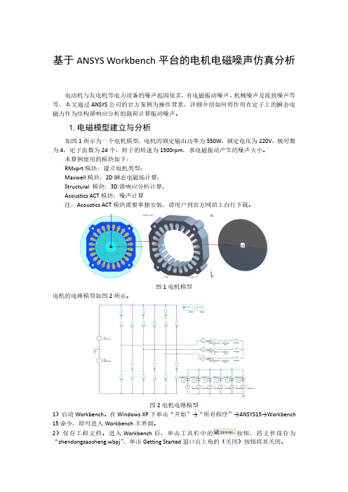
基于ANSYS Workbench平台的电机电磁噪声仿真分析电动机与发电机等电力设备的噪声起因很多,有电磁振动噪声、机械噪声及流致噪声等等,本文通过ANSYS公司的官方案例为操作背景,详细介绍如何将作用在定子上的瞬态电磁力作为结构谐响应分析的载荷计算振动噪声。
1.电磁模型建立与分析如图1所示为一个电机模型,电机的额定输出功率为550W,额定电压为220V,极对数为4,定子齿数为24个,转子的转速为1500rpm,求电磁振动产生的噪声大小。
本算例使用的模块如下:RMxprt模块:建立电机类型;Maxwell模块:2D瞬态电磁场计算;Structural模块:3D谐响应分析计算;Acoustics ACT模块:噪声计算注:Acoustics ACT模块需要单独安装,请用户到官方网站上自行下载。
图1电机模型电机的电路模型如图2所示。
图2电机电路模型1)启动Workbench。
在Windows XP下单击“开始”→“所有程序”→ANSYS15→Workbench 15命令,即可进入Workbench主界面。
2)保存工程文档。
进入Workbench后,单击工具栏中的按钮,将文件保存为“zhendongzaosheng.wbpj”,单击Getting Started窗口右上角的(关闭)按钮将其关闭。
3)双击Toolbox→Analysis System→RMxprt模块建立项目A,如图3所示。
4)双击项目A中的A1栏进如RMxprt电机设置平台,如图4所示。
图3RMxprt模块图4RMxprt平台5)依次选择菜单RMxprt→Machine Type,在弹出的电机类型选择对话框中单击Generic Rotating Machine选项,单击OK按钮,如图5所示。
6)单击Project Manager→RMxprt→Machine选项,在下面出现属性设置对话框中作如下设置:在Source Type栏中选择AC选项;在Structure栏中选择Inner Rotor选项;在Stator Type栏中选择SLOT_AC选项;在Rotor Type栏中选择PM_INTERIOR选项,如图6所示。
ANSYSWorkbench电磁场分析例子共38页

ANSYS, Inc. Proprietary
Contents
Workbench Electromagnetics
– Workbench Emag Roadmap
– Design Modeler
• Enclosure Symmetry • Winding bodies • Winding Tool
• Workbench v9.0 is the first release with electromagnetic analysis capability. – Support solid and stranded (wound) conductors – Automated computations of force, torque, inductance, and coil flux linkage. – Easily set up simulations to compute results as a function of current, stroke, or rotor angle.
– Up to 3 three symmetry planes can be specified. – Full or partial models can be included in the Enclosure. – During the model transfer from DesignModeler to Simulation, the enclosure feature with symmetry planes forms two kinds of named selections:
– Winding Bodies: Used to represent wound coils for source excitation. The advantage of these bodies is that they are not 3D CAD objects, and hence simplify modeling/meshing of winding structures.
ANSYS电磁场仿真实验报告

电磁场仿真实验报告求平行输电线周围的电位和电场分布一、报告要求:该生学号尾号为1,建立3条垂直排布的导线。
电位由下到上分别为1V,2V,3V,如下图所示:二、模型说明:静电场计算,求解区域为模型的5倍,截断边界条件。
最下方导线对地高度为10米,导线半径为0.01米,导线之间间距为5米。
(即:H1=10m,H2=15m,H3=20m,U1=1V,U2=2V,U3=3V,R0=0.01m,求解区域为一半圆,题目要求求解区域为模型的5倍,模型尺寸认为是40m,故取半圆半径L=200m。
)如下图所示:三、实验步骤:1、确定文件名,选择研究范围。
点击Utility Menu>File>Change Title,输入你的文件名。
例如“姓名_学号”(ZLM_2012301530051)点击Main Menu>Preferences,选择Electric。
点击Main Menu>Preprocessor>,进入前处理模块(command: /TITLE,ZLM_2012301530051/COM,Preferences for GUI filtering have been set to display:/COM, Electric/PREP7 )2、定义参数点击Utility Menu>Parameters>Scalar Parameters,在下面“Selection”空白区域填入参数:H1=10H2=15H3=20R0=0.01U1=1U2=2U3=3每一个参数输入完毕,点击“Accept ”按钮,输入的参数就导入上方“Items”指示的框中,等参数导入完毕后,点击“close”按钮关闭对话框。
(command: *SET,H1,10*SET,H2,15*SET,H3,20*SET,R0,0.01*SET,U1,1*SET,U2,2*SET,U3,3)3、定义单元类型点击Main Menu>Preprocessor>Element Type>Add/Edit/Delete,出现单元类型对话框“Element Types”,点击Add,弹出单元类型选择库对话框“Library of ElementTpes”选择Electrostatic 和2D Quad 121(二维四边形单元plane121)。
ANSYS Workbench 9.0电磁学教程实例(英文ppt)

© 2004 ANSYS, Inc.
ANSYS, Inc. Proprietary
Enclosure & Fill Tools
Design Modeler (DM) includes two features to allow a user to create a volumetric “field” body associated with a solid model.
ANSYS, Inc. Proprietary
Workbench Emag Markets
Target markets: • Solenoid actuators • Permanent magnet devices • Sensors • Rotating Electric machines
– Synchronous machines – DC machines – Permanent magnet machines
ANSYS Workbench 9.0 Electromagnetics
Paul Lethbridge
© 2004 ANSYS, Inc.
ANSYS, Inc. Proprietary
Contents
Workbench Electromagnetics
– Workbench Emag Roadmap
© 2004 ANSYS, Inc.
ANSYS, Inc. Proprietary
Enclosure Symmetry
•Feature: The Enclosure feature now supports symmetry models when the enclosure shape is a box or a cylinder:
- 1、下载文档前请自行甄别文档内容的完整性,平台不提供额外的编辑、内容补充、找答案等附加服务。
- 2、"仅部分预览"的文档,不可在线预览部分如存在完整性等问题,可反馈申请退款(可完整预览的文档不适用该条件!)。
- 3、如文档侵犯您的权益,请联系客服反馈,我们会尽快为您处理(人工客服工作时间:9:00-18:30)。
IntroductionThe Magnetic Valve includes a fixed and a rotating part. The rotating body has to move, as quickly as possible, to rest in one of the 2 possible stop positions. Driving current patterns are the input to generate suitable torques. The customer experienced different performances of the valve for different current patterns: sometimes he got strong bumps on the mechanic stops and failures of the valve behaviour. the customer decided to commit a simulation of the magnetic and dynamic behaviour of the valve, instead to build a prototype.Analysis GoalThe goal is ton achieve measure of the Magnetic Torque, as function of current and rotation angle within a parametric approachOwner:EnginsoftUsage Restrictions:Freely available for useIndustry:AutomotiveApplication:ValvePhysics:ElectromagneticsProduct(s)/Version:ANSYS-v10.1Geometry Type(s):SolidGeometry Format(s): Design ModelerModel Size:147070 Nodes, 105742 ElementsElement Type(s): Edge 117Estimated Demo Time:15 Minutes to show, 12 minutes running timeCustomer:Competition:Comsol,AnsoftChallenge:Free accurate Mesh, Parametric Model, Non LinearMagnetic AnalysisKey Features Used:Sphere of influence for meshing, BH Non Linear Curvedata import, Parametric AnalysisSteps and Points to Convey.Picture Guide.Start ANSYS Workbench Environment, and choose “New Geometry”.Importing of external geometrySet the desired length unit: meters.01) Click “File > Open > Import External Geometry File”.02) Click on “Generate” in order to confirm the importation of the geometry.The geometry regards a magnetic valve.Steps and Points to Convey.Picture Guide.Create a Parametric, Relative Rotation between two groups of bodies01) Create a local coordinate system (plane 4) by clicking on the “New Plane” icon in the tool bar.02) In “Details of Plane4 >. Type” choose from face in order to select the surface of interest. 03) Choose the space to the right of “Base Face” in Details of Plane4 and select the surface indicated in light blue in the plot at right.The local coordinate system “Plane 4” is now visible, centered on a face vertex04) In “Details of Plane4 >. Transform 1 (RMB)” insert an offset along X axis of –0.00825 m.05) In “Details of Plane4 >. Transform 1 (RMB)” insert an offset along Y axis of 0.0015 m.06) Click Generate to create Plane4Create another plane (Plane5).07) In “Details of Plane5 > Type” choose from plane. Base plane should be set to Plane4.08) In “Details of Plane5 >. Transform 1 (RMB)” insert a rotation about Z axis of 30°. 09) Click Generate to create Plane5.Steps and Points to Convey. Picture Guide.The local coordinate system “Plane 5” is now visible.10) From the tool bar menu, select “Tools > Freeze”.The freezing operation is indicated when bodies are displayed with transparency.11) From the tool bar menu, select “Create > Body Operation” set “Type” to “Move” click on the box to the right of Bodies.12) Select the bodies highlighted at right (use the Ctrl button to select multiple entities) and click Apply.Steps and Points to Convey.Picture Guide.13) In “Details of BodyOp1” choose the box to the right of “Source Plane” and pick on Plane4 in the Tree Outline.14) In a similar fashion, set “Destination Plane” to Plane5.Then click on “Generate” to move the parts as shown at right.ENCLOSURE definition01) From the tool bar menu, select “Tools >Enclosure” in order to insert a control volume cylindrically shaped and aligned to Y axis. Set the Cushion to 0.0375 m and set “Merge Parts?” to “Yes”.02) Click Generate to create the enclosureIn the “Outline” tree the just created enclosure is now visible.Steps and Points to Convey Picture GuideEnclosure is visible in the “Model View”window.CREATE the WINDING COIL01) In the Tree Outline, Open “1 Part, 7 Bodies > Part”. RMB on the last Solid in the list and choose “Hide Body” in the drop down menu. This will allow access to the surfaces of the imported geometry for forthcoming picking operations.02) Create a new plane (Plane6)03) In “Details of Plane6 >. Type” choose “From Face”.04) Click on the box to the right of “Base Face” and select the surface shown at right.05) In “Details of Plane6 >. Transform 1 (RMB)” insert an offset along Z axis of –0.0231 m.Click on Generate to create Plane6.06) With Plane6 now active, go to the tool bar and choose “New Sketch”.07) Select “Sketch1” in the “Tree Outline”.Steps and Points to Convey Picture Guide Sketching mode for winding coil generation08) Pick the Sketching tab at the bottom of theTree Outline09) Select “Circle” in the “Draw” window andchoose the center (origin of Plane6) and anarbitrary poin some distance away from thecenter to create a circle.10) Pick the Dimensions button at the bottom ofthe Sketching Toolboxes pane and choose“Radius”.11) Click on the circle and another arbitrarylocation for the radial dimension marker.12) In “Details of Sketch1”, modify the radiusR1 to be 0.00775 m.The sketch is now visible in the “Graphics”window.13) From the tool bar select “Concept > LineFrom Sketches”. Choose the circle and clickApply in the box to the right of “Base Objects”in “Details of Line1”. “Operation” should be setto “Add Material”.Click Generate.14) Choose the Line Body in the Tree Outline.15) In “Details of Line Body” set:•“Winding Body > Yes”•“Number of Turns” = 1•“CS Length” = 0.022 m•“CS Length” = 0.00375 mSteps and Points to ConveyPicture Guide16) From the tool bar, select “View > Show Cross Sections Solids”. The new winding body should appear as it does in the figure to the right.ANGLE as PARAMETER01) In the “Tree Outline” select “Plane5”02) Make the rotation about Z axis as parameter by clicking on the box to the left of “FD1, Value 1”.03) Rename the parameter as “angle”.Steps and Points to Convey.Picture Guide.04) From the tool bar, select “Tools > Options>Common Settings>Geometry Import”. Remove “DS” from the field to the right of “Personal Parameter Key” to remove the DS prefix naming convention restriction for importing parameters. Click OK.GO IN SIMULATIONIn the “[Project]” window, select “New Simulation”.In the “[Simulation]” window, the “Outline” tree should be as in figure.Steps and Points to ConveyPicture GuideMaterials Properties DefinitionSelect “Data” in the tool bar to open the “[Engineering Data]” window.Materials Properties Definitionchange defaults of STRUCTURAL STEEL01) Select “Structural Steel” and click on “Add/Remove Properties” in the “Electromagnetics” field and unselect the following items:- “Relative Permeability” - “Resistivity”02) Check the box to the left of “B-H curve” and click OK.03) Say “Yes” to the “Remove Material Properties” box that appears.04) Open excel file “bh1.xls” and copy the two data columns (highlight them with the mouse cursor and type Cntl-C).Steps and Points to ConveyPicture Guide05) Click the icon depicting an xy plot to the right of “B-H Curve”06) LMB on the 2 (second row) of the “Magnetic Flux Density vs. Magnetic Field Intensity” table and press “Ctrl +V” to paste the two column data from the .xls file.07) Click on the B-H Curve icon at the lower right.The curve should appear as shown at right.NEW Material definition IRONRMB on “Materials (2)” in the tree and choose “Insert New Material”. RMB on “New Material”, choose Rename and change the name of the new material to Iron. Define BH data as before but this time use data from “bh2.xls” file.NEW Material definition NEODYMIUM01) Define a New material named “Neodymium”.02) Among Electromagnetics properties let active just: “Linear Hard Material”: 03) Insert the following data:• Cohercive Force: 7.9577 e5 A/m • Residual Induction 1.2 T01) Return to the Simulation Tab02) In the Outline Tree, open Geometry>Part and use the Cntl button to select both of the RIC9512_105 items. The parts should be highlighted as shown at right.03) In Details of “Multiple Selection”, changematerial from “Structural Steel” to “Iron”Steps and Points to ConveyPicture Guide04) Select the part shown at right.05) Change material from “Structural Steel” to “Neodymium”MESH01) Select the coil support solid (see figure)02) RMB on “Mesh” on the tree to insert a sizing control: Element Size 2e-303) Insert another sizing control , 1e-3, referred to 5 bodies as in the following picture. It may help to hide the 4th solid (the “air enclosure) in the Outline tree to simplify selecting these parts.Steps and Points to ConveyPicture Guide5 bodies for sizing setting n.204) In the Outline tree, RMB on Model and insert a “Coordinate Systems” branch. RMB on the Coordinate Systems branch and insert (define) a new Coordinate System. Choose “Origin” in the Details of “Coordinate System” pane, select the surface shown at right, and click Apply.05) RMB on Mesh in the Outline to insert a third sizing control:For “Type”, choose “Sphere of Influence”• Sphere Center: Coordinate System (defined just before) • Radius 1.5e-2 • Element size 5e-4Areas to be applied are the following (10 areas)Steps and Points to ConveyPicture Guide10 Areas where to apply the Sphere of Influence sizing control06) Click on Mesh -> Preview MeshThe Mesh should result as in figure, if the “Air” solid enclosure body is hideLOADSSet the Conductor Current value in details window related to “Conductor Winding Body”: 1000 ABOUNDARY CONDITIONSRMB on Environment in the tree and insert a Magnetic Flux Parallel object. Use the Cntl button to select the 3 exterior surfaces of the enclosure and click Apply.Steps and Points to Convey.Picture Guide.POSTPROCESSING SETTINGS01) Insert under the “Solution” tree the following output requests: • Total Flux Density • Total Flux Intensity 02) Select 3 bodies as in figure03) Insert a “Directional Force/Torque” output request with details:• In Details of “Directional Force/Torque” pane, change “Global Coordinate System” to “Coordinate System” (this is the user-defined coordinate system centered on the top surface of the permanent magnet).• Set Orientation to Y Direction (rotation axis)04) repeat Directional Force/Torque Request for both X and Z axis direction05) By a right click under the Solution Tree Insert a “Solution Information” request to monitor the run during the solutionSOLVE01) Highlight the Environment tree tosee/check all Boundary & Loads previously defined.02) Click on the “SOLVE” Icon to launchthe run.Solution times takes about 12 minutes on a 2.8 Ghz single processor 32bit PCSteps and Points to ConveyPicture GuideREVIEW RESULTS01) See the Total Flux of Magnetic results 02) Set up a Vector Image of the MagneticField03) After Vector Image settings show a Vector Plot of Magnetic Field03)See the Magnetic Force distribution, Yaxis direction, on the requested parts. 04)The same for X, Z directions05)Activate the view from Y Global Axis06)Define a “Slice Plane”07)Draw the slice plane trace at nearlyalong the Y global direction08)View from the X Global direction09)Activate “show elements” and show themagnetic fieldSteps and Points to Convey Picture GuideSET UP A PARAMETRIC ANALYSIS01) Click on “Model”02) Click on CAD Parameters Detail toactivate the “angle” as a parameter. Thiswill be the first INPUT parameter.03) Click on Environment and Duplicate byright click04) Activate the Conductor Current Value asparameter. This is the second INPUTparameter n.2.05) Activate the Torque value in Y directionas OUTPUT parameter (ThirdParameter)06)Click on “Solution” of Environment 2and then click on Parameter Manager 07)Set up many cases as you like, forexample with 4 current values, 3 values other than the previously solved.。