matlab中的图像增强实验附程序代码
MATLAB图像增强总结程序
MATLAB图像增强程序举例1.灰度变换增强程序:% GRAY TRANSFORMclc;I=imread('pout.tif');imshow(I);J=imadjust(I,[0.3 0.7],[0 1],1); %transforms the walues in the %intensity image I to values in J by linealy mapping %values between 0.3 and 0.7 to values between 0 and 1. figure;imshow(J);J=imadjust(I,[0.3 0.7],[0 1],0.5); % if GAMMA is less than 1,the mapping si weighted to ward higher (brighter)%output values.figure;imshow(J);J=imadjust(I,[0.3 0.7],[0 1],1.5); % if GAMMA is greater than 1,the mapping si weighted toward lower (darker)%output values.figure;imshow(J)J=imadjust(I,[0.3 0.7],[0 1],1); % If TOP<BOTTOM,the output image is reversed,as in a p hotographic negative.figure;imshow(J);2.直方图灰度变换%直方图灰度变换[X,map]=imread('forest.tif');I=ind2gray(X,map);%把索引图像转换为灰度图像imshow(I);title('原图像');improfile%用鼠标选择一条对角线,显示线段的灰度值figure;subplot(121)plot(0:0.01:1,sqrt(0:0.01:1))axis squaretitle('平方根灰度变换函数')subplot(122)maxnum=double(max(max(I)));%取得二维数组最大值J=sqrt(double(I)/maxnum);%把数据类型转换成double,然后进行平方根变换%sqrt函数不支持uint8类型J=uint8(J*maxnum);%把数据类型转换成uint8类型imshow(J)title('平方根变换后的图像')3.直方图均衡化程序举例% HISTGRAM EAQUALIZATIONclc;% Clear command windowI=imread('tire.tif');% reads the image in tire.tif into Iimshow(I);% displays the intensity image I with 256 gray levels figure;%creates a new figure windowimhist(I);% displays a histogram for the intensity image IJ=histeq(I,64);% transforms the intensity image I,returning J an intensity figure;%image with 64 discrete levelsimshow(J);figure;imhist(J);J=histeq(I,32);%transforms the intensity image ,returning in % J an intensity figure;%image with 32 discrete levelsimshow(J);figure;imhist(J);4.直方图规定化程序举例% HISTGRAM REGULIZATIONclc;%Clear command windowI=imread('tire.tif');%reads the image in tire.tif into IJ=histeq(I,32);%transforms the intensity image I,returning in%J an intensity image with 32 discrete levels[counts,x]=imhist(J);%displays a histogram for the intensity image IQ=imread('pout.tif');%reads the image in tire.tif into Ifigure;imshow(Q);figure;imhist(Q);M=histeq(Q,counts);%transforms the intensity image Q so that the%histogram of the output image M approximately matches counts figure;imshow(M);figure;imhist(M);空域滤波增强部分程序1.线性平滑滤波I=imread('eight.tif');J=imnoise(I,'salt & pepper',0.02);subplot(221),imshow(I)title('原图像')subplot(222),imshow(J)title('添加椒盐噪声图像')K1=filter2(fspecial('average',3),J)/255;%应用3*3邻域窗口法subplot(223),imshow(K1)title('3x3窗的邻域平均滤波图像')K2=filter2(fspecial('average',7),J)/255;%应用7*7邻域窗口法subplot(224),imshow(K2)title('7x7窗的邻域平均滤波图像')2.中值滤波器MATLAB中的二维中值滤波函数medfit2来进行图像中椒盐躁声的去除%IMAGE NOISE REDUCTION WITH MEDIAN FILTERclc;hood=3;%滤波窗口[I,map]=imread('eight.tif');imshow(I,map);noisy=imnoise(I,'salt & pepper',0.05);figure;imshow(noisy,map);filtered1=medfilt2(noisy,[hood hood]);figure;imshow(filtered1,map);hood=5;filtered2=medfilt2(noisy,[hood hood]);figure;imshow(filtered2,map);hood=7;filtered3=medfilt2(noisy,[hood hood]);figure;imshow(filtered3,map);3. 4邻域8邻域平均滤波算法% IMAGE NOISE REDUCTION WITH MEAN ALGORITHM clc;[I,map]=imread('eight.tif');noisy=imnoise(I,'salt & pepper',0.05);myfilt1=[0 1 0;1 1 1;0 1 0];%4邻域平均滤波模版myfilt1=myfilt1/9;%对模版归一化filtered1=filter2(myfilt1,noisy);imshow(filtered1,map);myfilt2=[1 1 1;1 1 1;1 1 1];myfilt2=myfilt2/9;filtered2=filter2(myfilt2,noisy);figure;imshow(filtered2,map);频域增强程序举例1.低通滤波器% LOWPASS FILTERclc;[I,map]=imread('eight.tif');noisy=imnoise(I,'gaussian',0.05);imshow(noisy,map);myfilt1=[1 1 1;1 1 1;1 1 1];myfilt1=myfilt1/9;filtered1=filter2(myfilt1,noisy);figure;imshow(filtered1,map);myfilt2=[1 1 1;1 2 1;1 1 1];myfilt2=myfilt2/10;filtered2=filter2(myfilt2,noisy); figure;imshow(filtered2,map);myfilt3=[1 2 1;2 4 2; 1 2 1]; myfilt3=filter2(myfilt3,noisy); figure;imshow(filtered3,map);2.布特沃斯低通滤波器图像实例I=imread('saturn.png');J=imnoise(I,'salt & pepper',0.02); subplot(121),imshow(J)title('含噪声的原图像')J=double(J);f=fft2(J);g=fftshift(f);[M,N]=size(f);n=3;d0=20;n1=floor(M/2);n2=floor(N/2);for i=1:M;for j=1:N;d=sqrt((i-n1)^2+(j-n2)^2);h=1/(1+0.414*(d/d0)^(2*n));g(i,j)=h*g(i,j);endendg=ifftshift(g);g=uint8(real(ifft2(g)));subplot(122),imshow(g)title('三阶Butterworth滤波图像')色彩增强程序举例1.真彩色增强实例:%真彩色图像的分解clc;RGB=imread('peppers.png');subplot(221),imshow(RGB)title('原始真彩色图像')subplot(222),imshow(RGB(:,:,1))title('真彩色图像的红色分量')subplot(223),imshow(RGB(:,:,2))title('真彩色图像的绿色分量')subplot(224),imshow(RGB(:,:,3))2.伪彩色增强举例:I=imread('cameraman.tif');imshow(I);X=grayslice(I,16);%thresholds the intensity image I using%threshold values 1/16,2/16,…..,15/16,returning an indexed %image in X figure;imshow(X,hot(16));3.假彩色增强处理程序举例[RGB]=imread('ghost.bmp');imshow(RGB);RGBnew(:,:,1)=RGB(:,:,3);RGBnew(:,:,2)=RGB(:,:,1);RGBnew(:,:,3)=RGB(:,:,2);figure;subplot(121);imshow(RGB);subplot(122);imshow(RGBnew);主要转载自:/s/blog_488c87020100cice.htm l。
实验二图像增强

实验二图像增强一、目的1.熟悉并学会使用MATLAB中图像增强的相关函数;2.了解图像增强的方法,噪声去除的方法和去噪效果。
二、实验内容1.利用MATLAB函数读和显示图像;2.对图像增加噪声;3.用不同方法去噪:如平滑、中值滤波增加噪声程序:I=imread('autumn.tif');subplot(311)imshow(I) ;title('原图')%叠加均值为0,方差为0.02的高斯噪声subplot(312)J1=imnoise(I,'gaussian',0,0.02);%imnoise函数归一化原因,很小方差但效果很明显imshow(J1);title('加高斯白噪声图')%叠加密度为0.04的椒盐噪声subplot(313)J2=imnoise(I,'salt & pepper',0.3);imshow(J2);title('加椒盐噪声图')imwrite(J1,'autumn_gaussian.tif');imwrite(J2,'autumn_saltpepper.bmp');线性平滑滤波程序:%线性平滑滤波I=imread('eight.tif');J=imnoise(I,'salt & pepper',0.02);subplot(221),imshow(I)title('原图像')subplot(222),imshow(J)title('添加椒盐噪声图像')K1=filter2(fspecial('average',3),J)/255;%应用3X3领域窗口法subplot(223),imshow(K1)title('3X3窗的领域平均滤波图像')K2=filter2(fspecial('average',7),J)/255;%应用7X7领域窗口法subplot(224),imshow(K2)title('7X7窗的领域平均滤波图像')中值滤波程序:clc%中值滤波hood=3; %滤波窗口[I,map]=imread('eight.tif');subplot(151)imshow(I,map);title('原图像')noisy=imnoise(I,'salt & pepper',0.05); subplot(152)imshow(noisy,map);title('加椒盐噪声像')filtered1=medfilt2(noisy,[hood hood]); subplot(153),imshow(filtered1,map);title('33去噪')hood=5;filtered2=medfilt2(noisy,[hood hood]); subplot(154)imshow(filtered2,map);title('55去噪')hood=7;filtered3=medfilt2(noisy,[hood hood]); subplot(155)imshow(filtered3,map); title('77去噪')。
基于MATLAB的图像增强处理
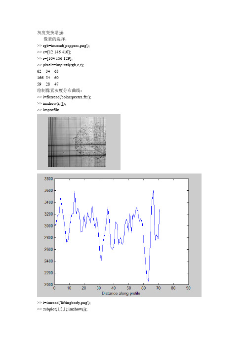
灰度变换增强:像素的选择:>> rgb=imread('peppers.png'); >> c=[12 146 410];>> r=[104 156 129];>> pixels=impixel(rgb,c,r);62 34 63166 54 6059 28 47绘制像素灰度分布曲线:>> i=fitsread('solarspectra.fts'); >> imshow(i,[]);>> improfile>> i=imread('liftingbody.png'); >> subplot(1,2,1);imshow(i);>> x=[19 427 416 77];>> y=[96 462 37 33];>> subplot(1,2,2);improfile(i,x,y); >> grid on;绘制图像的等值线:>> i=imread('circuit.tif'); >> subplot(1,2,1);imshow(i); >> subplot(1,2,2);imcontour(i,3);直方图:>> i=imread('pout.tif');>> subplot(1,2,1);imshow(i); >> subplot(1,2,2);imhist(i);图像像素的统计特性:>> i=imread('pout.tif'); >> b=mean2(i)b =110.3037>> c=std2(i)c =23.1811>> j=medfilt2(i);>> r=corr2(i,j)r =0.9959图像的区域属性:>> bw=imread('text.png'); >> l=bwlabel(bw);>> stats=regionprops(l,'all');>> stats(23)ans =Area: 48Centroid: [121.3958 15.8750]BoundingBox: [118.5000 8.5000 6 14]SubarrayIdx: {[9 10 11 12 13 14 15 16 17 18 19 20 21 22] [119 120 121 122 123 124]}MajorAxisLength: 15.5413MinorAxisLength: 5.1684Eccentricity: 0.9431Orientation: -87.3848ConvexHull: [10x2 double]ConvexImage: [14x6 logical]ConvexArea: 67Image: [14x6 logical]FilledImage: [14x6 logical]FilledArea: 48EulerNumber: 1Extrema: [8x2 double]EquivDiameter: 7.8176Solidity: 0.7164Extent: 0.5714PixelIdxList: [48x1 double]PixelList: [48x2 double]灰度变换:线性变换:>> x=imread('forest.tif');>> f0=0;g0=0;>> f1=10;g1=10;>> f2=180;g2=1800;>> f3=255;g3=255;>> figure;plot([f0,f1,f2,f3],[g0,g1,g2,g3]);>> axis tight;>> r1=(g1-g0)/(f1-f0);>> b1=g0-r1*f0;>> r2=(g2-g1)/(f2-f1);>> b2=g1-r2*f1;>> r3=(g3-g2)/(f3-f2);>> b3=g2-r3*f2;>> [m,n]=size(x);>> x1=double(x);>> for i=1:mfor j=1:nf=x1(i,j);g(i,j)=0;if(f>=f1)&(f<=f2)g(i,j)=r1*f+b2;else if(f>=f2)&(f<=f3)g(i,j)=r3*f+b3;end;end;end;end;>> figure;imshow(mat2gray(g))分段线性变换:>> x=imread('forest.tif');>> f0=0;g0=0;>> f1=50;g1=50;>> f2=220;g2=250;>> f3=255;g3=255;>> subplot(1,2,1);plot([f0,f1,f2,f3],[g0,g1,g2,g3]); >> axis tight;>> r1=(g1-g0)/(f1-f0);>> b1=g0-r1*f0;>> r2=(g2-g1)/(f2-f1);>> b2=g1-r2*f1;>> r3=(g3-g2)/(f3-f2);>> b3=g2-r3*f2;>> [m,n]=size(x);>> x1=double(x);>> for i=1:mfor j=1:nf=x1(i,j);g(i,j)=0;if(f>=f1)&(f<=f2)g(i,j)=r1*f+b2;else if(f>=f2)&(f<=f3)g(i,j)=r3*f+b3;end;end;end;end;>> subplot(1,2,2);imshow(mat2gray(g));非线性灰度变换:>> x=imread('forest.tif');>> c=255/log(256);>> x=0:255;>> y=c*log(1+x);>> subplot(1,2,1);plot(x,y);axis tight; >> [m,n]=size(x);>> x1=double(x);>> for i=1:mfor j=1:ng(i,j)=0;g(i,j)=c*log(x1(i,j)+1);end;end;>> subplot(1,2,2);imshow(mat2gray(g));对灰度图像进行灰度值调整:>> p=imread('pout.tif');>> pj=imadjust(p);>> ph=histeq(p);>> pa=adapthisteq(p);>> subplot(1,2,1);imshow(p);>> subplot(1,2,2);imshow(pj);对索引图像进行灰度值调整:>> rgb1=imread('football.jpg');>> rgb2=imadjust(rgb1,[.2 .3 0;.6 .7 1],[]);>> subplot(1,2,1);imshow(rgb1);>> subplot(1,2,2);imshow(rgb2);增加图像的亮度:>> rgb1=imread('football.jpg');>> rgb2=imadjust(rgb1,[.2 .3 0;.6 .7 1],[]);>> subplot(1,2,1);imshow(rgb1);>> subplot(1,2,2);imshow(rgb2);>> clear;>> figure('Renderer','zbuffer');axesm bries;>> text(1.2,-1.8,'Briesemeister projection');>> framem('FlineWidth',1);>> load topo;>> geoshow(topo,topolegend,'DisplayType','texturemap'); >> demcmap(topo);>> set(gcf,'color','w');>> brighten(.5);直方图均衡化:>> i=imread('tire.tif');>> j=histeq(i);>> subplot(2,2,1);imshow(i); >> subplot(2,2,2);imshow(j); >> subplot(2,2,3);imhist(i,64); >> subplot(2,2,4);imhist(j,64);直方图的规定化:>> i=imread('forest.tif');>> h=0:255;>> subplot(2,2,1);imshow(i); >> j=histeq(i,h);>> subplot(2,2,2);imshow(j); >> subplot(2,2,3);imhist(i,64); >> subplot(2,2,4);imhist(j,64);空域滤波增强:平滑滤波器:>> i=imread('cameraman.tif'); >> subplot(2,2,1);imshow(i); >> h=fspecial('motion',20,45); >> mb=imfilter(i,h,'replicate'); >> subplot(2,2,2);imshow(mb); >> h=fspecial('disk',10);>> bl=imfilter(i,h,'replicate'); >> subplot(2,2,3);imshow(bl); >> h=fspecial('unsharp');>> sh=imfilter(i,h,'replicate'); >> subplot(2,2,4);imshow(sh);用各种尺寸的模板平滑图像:>> i=imread('eight.tif');>> j=imnoise(i,'salt & pepper',0.025); >> subplot(2,3,1);imshow(i);>> subplot(2,3,2);imshow(j);>> k1=filter2(fspecial('average',3),j); >> k2=filter2(fspecial('average',5),j); >> k3=filter2(fspecial('average',7),j); >> k4=filter2(fspecial('average',9),j); >> subplot(2,3,3);imshow(uint8(k1)); >> subplot(2,3,4);imshow(uint8(k2)); >> subplot(2,3,5);imshow(uint8(k3)); >> subplot(2,3,6);imshow(uint8(k4));中值滤波器:>> i=imread('cameraman.tif'); >> j1=imnoise(i,'salt & pepper',0.01); >> k1=medfilt2(j1);>> j2=imnoise(i,'gaussian',0.01); >> k2=medfilt2(j2);>> subplot(2,3,1);imshow(i);>> subplot(2,3,2);imshow(j1);>> subplot(2,3,3);imshow(k1);>> subplot(2,3,4);imshow(j2);>> subplot(2,3,5);imshow(k2);>> i=imread('cameraman.tif');>> j1=imnoise(i,'salt & pepper',0.01); >> k1=medfilt2(j1,[6,6]);>> j2=imnoise(i,'gaussian',0.01); >> k2=medfilt2(j2,[6,6]);>> subplot(2,3,1);imshow(i);>> subplot(2,3,2);imshow(j1);>> subplot(2,3,3);imshow(k1,[]); >> subplot(2,3,4);imshow(i);>> subplot(2,3,5);imshow(j2);>> subplot(2,3,6);imshow(k2,[]);带噪声的图像的最小值与最大值滤波图像:>> a=imread('eight.tif');>> b=imnoise(a,'salt & pepper',0.025);>> do=[0 0 1 0 0;0 1 0 1 0;1 0 1 0 1;0 1 0 1 0;0 0 1 0 0]; >> c=ordfilt2(b,1,do);>> d=ordfilt2(b,9,do);>> subplot(2,2,1);imshow(a);>> subplot(2,2,2);imshow(b);>> subplot(2,2,3);imshow(c);>> subplot(2,2,4);imshow(d);自适应滤波器:>> rgb=imread('saturn.png'); >> i=rgb2gray(rgb);>> j=imnoise(i,'gaussian',0,0.025); >> k=wiener2(j,[5 5]);>> subplot(1,3,1);imshow(i); >> subplot(1,3,2);imshow(j); >> subplot(1,3,3);imshow(k);锐化滤波器:线性锐化滤波器:>> i=imread('rice.png');>> h=fspecial('laplacian');>> i2=filter2(h,i);>> subplot(1,2,1);imshow(i); >> subplot(1,2,2);imshow(i2);非线性锐化滤波器:>> [i,map]=imread('eight.tif'); >> subplot(2,2,1);imshow(i,map); >> i=double(i);>> [ix,iy]=gradient(i);>> gm=sqrt(ix.*ix+iy.*iy);>> out1=gm;>> subplot(2,2,2);imshow(out1,map); >> out2=i;>> j=find(gm>=15);>> out2(j)=gm(j);>> subplot(2,2,3);imshow(out2,map); >> out3=i;>> j=find(gm>=20);>> out3(j)=255;>> q=find(gm<20);>> out3(q)=0;>> subplot(2,2,4);imshow(out3,map);>> i=imread('eight.tif');>> subplot(2,2,1);imshow(i); >> h1=fspecial('sobel');>> i1=filter2(h1,i);>> h2=fspecial('prewitt'); >> i2=filter2(h2,i);>> h3=fspecial('log');>> i3=filter2(h3,i);>> subplot(2,2,2);imshow(i1); >> subplot(2,2,3);imshow(i2); >> subplot(2,2,4);imshow(i3);频域滤波增强:低通滤波:>> i1=imread('eight.tif');>> i2=imnoise(i1,'salt & pepper'); >> f=double(i2);>> g=fft2(f);>> g=fftshift(g);>> [N1,N2]=size(g);>> n=2;>> d0=50;>> n1=fix(N1/2);>> n2=fix(N2/2);>> for i=1:N1for j=2:N2d=sqrt((i-n1)^2+(j-n2)^2);h=1/(1+0.414*(d/d0)^(2*n));s1(i,j)=h*g(i,j);if(g(i,j)>50)s2(i,j)=0;elses2(i,j)=g(i,j);end;end;end;>> s1=ifftshift(s1);>> s2=ifftshift(s2);>> x2=ifft2(s1);>> x3=uint8(real(x2));>> x4=ifft2(s2);>> x5=uint8(real(x4));>> subplot(2,2,1);imshow(i1); >> subplot(2,2,2);imshow(i2); >> subplot(2,2,3);imshow(x3); >> subplot(2,2,4);imshow(x5);高通滤波器:>> j=imread('rice.png');>> subplot(2,3,1);imshow(uint8(j)); >> j=double(j);>> f=fft2(j);>> g=fftshift(f);>> [M,N]=size(f);>> n1=floor(M/2);>> n2=floor(N/2);>> d0=20;>> for i=1:Mfor j=1:Nd=sqrt((i-n1)^2+(j-n2)^2);if d>=d0h1=1;h2=1+0.5;elseh1=0;h2=0.5;end;g1(i,j)=h1*g(i,j);g2(i,j)=h2*g(i,j);end;end;>> g1=ifftshift(g1);>> g1=uint8(real(ifft2(g1)));>> g2=ifftshift(g2);>> g2=uint8(real(ifft2(g2)));>> subplot(2,3,2);imshow(g1);>> subplot(2,3,3);imshow(g2);>> n=2;>> d0=20;>> for i=1:Mfor j=1:Nd=sqrt((i-n1)^2+(j-n2)^2);if d==0h1=0;h2=.5;elseh1=1/(1+(d0/d)^(2*n));h2=1/(1+(d0/d)^(2*n))+0.5;end;gg1(i,j)=h1*g(i,j);gg2(i,j)=h2*g(i,j);end;end;>> gg1=ifftshift(gg1);>> gg1=uint8(real(ifft2(gg1)));>> gg2=ifftshift(gg2);>> gg2=uint8(real(ifft2(gg2)));>> subplot(2,3,4);imshow(gg1);>> subplot(2,3,5);imshow(gg2);同态滤波器:>> i=imread('eight.tif');>> j=double(i);>> f=fft2(j);>> g=fftshift(f);>> [M,N]=size(f);>> d0=10;>> r1=0.5;>> rh=2;>> c=4;>> n1=floor(M/2);>> n2=floor(N/2);>> for i=1:Mfor j=1:Nd=sqrt((i-n1)^2+(j-n2)^2);h=(rh-r1)*(1-exp(-c*(d.^2/d0.^2)))+r1;end;end;>> g=ifftshift(g);>> g=uint8(real(ifft2(g)));>> subplot(1,2,1);imshow(i);>> subplot(1,2,2);imshow(g);彩色增强:利用密度分割法进行伪彩色增强:>> a=imread('eight.tif');>> subplot(1,2,1);imshow(a);>> c=zeros(size(a));>> pos=find(a<20);>> c(pos)=a(pos);>> b(:,:,3)=c;>> c=zeros(size(a));>> pos=find((a>20)&(a<40));>> c(pos)=a(pos);>> b(:,:,2)=c;>> c=zeros(size(a));>> pos=find(a>=40);>> c(pos)=a(pos);>> b(:,:,1)=c;>> b=uint8(b);>> subplot(1,2,2);imshow(b);真彩色增强:>> rgb=imread('peppers.png');>> subplot(2,2,1);imshow(rgb); >> subplot(2,2,2);imshow(rgb(:,:,1)); >> subplot(2,2,3);imshow(rgb(:,:,2)); >> subplot(2,2,4);imshow(rgb(:,:,3));。
MATLAB常用图像增强方法(精)

M A T L A B常用图像增强方法(精)-CAL-FENGHAI.-(YICAI)-Company One1数字图像处理实验报告实验名称:常用图像增强方法专业班级: 07级电子信息工程2班姓名:王超学号:一、实验目的1、熟悉并掌握MATLAB图像处理工具箱的使用;2、理解并掌握常用的图像的增强技术。
二、实验步骤1、显示图像直方图选择一幅图像,转化为灰度图像后显示其直方图,建立M文件程序如下:a=imread('f:\';b=rgb2gray(a;subplot(1,2,1;imshow(b;subplot(1,2,2;imhist(b结果如图:2、直方图均衡化建立M文件,程序如下:a=imread('f:\';b=rgb2gray(a;subplot(1,3,1;imshow(b; subplot(1,3,2;imhist(b;c=histeq(b,64;[c,T]=histeq(b;subplot(1,3,3;imhist(c结果如图:3、采用二维中值滤波函数medfilt2对受椒盐噪声干扰的图像滤波,窗口分别采用3*3,5*5,7*7建立M文件程序如下:a=imread('f:\';x=rgb2gray(a;b=imnoise(x,'salt & pepper', ;subplot(2,2,1;imshow(b;c=medfilt2(b,[3 3];subplot(2,2,2;imshow(c;d=medfilt2(b,[5 5];subplot(2,2,3;imshow(d;e=medfilt2(b,[7 7];subplot(2,2,4;imshow(e结果如图:1图为加噪图像,2、3、4图分别为窗口采用3*3、5*5、7*7的滤波后的图像4、采用MATLAB中的函数filter2对受噪声干扰的图像进行均值滤波建立M文件程序如下:a=imread('f:\';b=rgb2gray(a;subplot(1,2,1;imshow(b;h=[1,2,1;0,0,0;-1,-2,-1];c=filter2(h,b;subplot(1,2,2;imshow(c结果如图:5、采用三种不同算子对图像进行锐化处理建立M文件如下:a=imread('f:\';b=rgb2gray(a;subplot(2,2,1;imshow(b;h=[1,2,1;0,0,0;-1,-2,-1]; %Sobel算子c=filter2(h,b;subplot(2,2,2;imshow(c ;d=double(b;h=[0,1,0;1,-4,0;0,1,0]; %拉氏算子e=conv2(d,h,'same';subplot(2,2,3;imshow(e ;h=[1,1,1;0,0,0;-1,-1,-1]; %Prewitt算子f=filter2(h,b;subplot(2,2,4;imshow(f结果如图:1图为原图的灰度图像;2图为经Sobel算子锐化处理后的图像;3图为经拉氏算子锐化处理后的图像;4图为经Prewitt算子锐化处理的图像三、实验总结1、不同平滑滤波器的处理效果,及其优缺点二维中值滤波器的窗口形式有多种,比如线状、方形等等。
图像处理的MATLAB实现实验一 空域图像增强
图像处理的MATLAB 实现实验一 空域图像增强一、实验目的(1)掌握基本的空域图像增强方法,观察图像增强的效果,加深理解;(2)了解空域平滑模板的特性及其对不同噪声的影响;(3)了解空域锐化模板的特性及其对边缘的影响。
二、实验内容(1)直方图处理:直方图均衡(2)空域平滑:均值滤波、中值滤波;三、实验要求(1)用matlab 语言进行仿真实验;(2)递交实验报告,要求给出实验原理、源程序、实验结果及分析。
四、具体实验内容及要求4.1 实验内容4.1.1 直方图均衡(1)读入原图像pollen.png 并显示原图像以及直方图(2)对原图像进行直方图均衡处理(3)显示均衡后图像以及直方图。
4..1.2 图像空域平滑(1)读入原图像lena.bmp 并显示;(2)对原图像分别添加高斯噪声和椒盐噪声,并显示加噪图像;(3)采用均值滤波进行去噪处理,并显示去噪图像;(4)采用中值滤波进行去噪处理,并显示去噪图像。
4.1.3 空域锐化(1)读入原图像bridge.gif 并显示;(2)采用sobel 算子对图像进行处理,并显示结果;(3)尝试采用其他锐化模板进行处理。
4.2 实验原理4.2.1 直方图均衡实验原理对图像像素个数多的灰度级进行展宽,而对图像中像素个数少的灰度级进行压缩。
而且,输入灰度级r 与输出灰度级s 的概率密度函数()r p r 和()s p s 有如下关系()()ds dr r p s p r s = 积分形式如下()()()dw w p L r T s rr ⎰-==01 4.2.2 图像滤波 (1)、椒盐噪声的中值滤波由于椒盐噪声的出现使该点的像素比周围的亮或暗许多,如果在某个模板中,对像素由小到大重新排列,那么最暗或最亮的点一定被排在两侧,取模板中间位置的灰度值像素代替待处理图像像素的灰度值,从而达到滤除噪声的目的。
(2)、高斯噪声的均值滤波均值滤波是一种空域线性的滤波方法,用像素邻域内各像素的灰度平均值代替该像素原来的灰度值;均值滤波采用的是模板操作,将模板在图像中从左到右,从上到下的顺序移动将模板中心与每个像素重合;将模板中个系数与其对应的像素一并相乘,然后再经所有的结果一并相加;将上面相加的结果重新付给模板中心对应的像素点,那么该灰度值,就是经均值滤波后平滑后的灰度值。
图像增强实验及MATLAB在图像处理中的一些函数资料
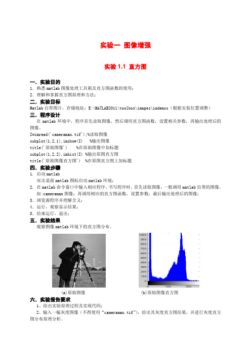
实验一图像增强实验1.1 直方图一.实验目的1.熟悉matlab图像处理工具箱及直方图函数的使用;2.理解和掌握直方图原理和方法;二.实验目标Matlab自带图片,存储地址:E:\MATLAB2011\toolbox\images\imdemos(根据安装位置调整)三.程序设计在matlab环境中,程序首先读取图像,然后调用直方图函数,设置相关参数,再输出处理后的图像。
I=imread('cameraman.tif');%读取图像subplot(1,2,1),imshow(I) %输出图像title('原始图像') %在原始图像中加标题subplot(1,2,2),imhist(I) %输出原图直方图title('原始图像直方图') %在原图直方图上加标题四.实验步骤1. 启动matlab双击桌面matlab图标启动matlab环境;2. 在matlab命令窗口中输入相应程序。
书写程序时,首先读取图像,一般调用matlab自带的图像,如:cameraman图像;再调用相应的直方图函数,设置参数;最后输出处理后的图像;3.浏览源程序并理解含义;4.运行,观察显示结果;5.结束运行,退出;五.实验结果观察图像matlab环境下的直方图分布。
(a)原始图像 (b)原始图像直方图六.实验报告要求1、给出实验原理过程及实现代码;2、输入一幅灰度图像(不得使用“cameraman.tif”),给出其灰度直方图结果,并进行灰度直方图分布原理分析。
1、实验原理过程:每一张图片都是一张灰度图片,都是由一些像素点组成,matlab 读取图片,并显示该图片的灰度级范围。
实现代码:I=imread('D:\MATLAB7\toolbox\images\imdemos\rice.png');%读取图像 subplot(1,2,1),imshow(I) %输出图像 subplot(1,2,2),imhist(I) %输出原图直方图title('原始图像直方图') %在原图直方图上加标题 2、0100200原始图像直方图实验1.2 灰度均衡化一.实验目的1.熟悉matlab 图像处理工具箱中灰度均衡函数的使用; 2.理解和掌握灰度均衡原理和实现方法;二.实验设备1.PC 机一台;2.软件matlab ;三.程序设计在matlab 环境中,程序首先读取图像,然后调用灰度均衡函数,设置相关参数,再输出处理后的图像。
图像增强的matlab源代码带注释
代码一:% 2.灰度线性变换,利用imadjust函数对图像局部灰度范围进行扩展% MATLAB 程序实现如下:I=imread('e.jpg');subplot(2,2,1),imshow(I);title('原始图像');axis([50,250,50,200]);axis on; %显示坐标系I1=rgb2gray(I); %图像I必须为彩色图像subplot(2,2,2),imshow(I1);title('灰度图像');axis([50,250,50,200]);axis on; %显示坐标系J=imadjust(I1,[0.1 0.5],[]); %局部拉伸,把[0.1 0.5]内的灰度拉伸为[0 1] subplot(2,2,3),imshow(J);title('线性变换图像[0.1 0.5]');axis([50,250,50,200]);grid on; %显示网格线axis on; %显示坐标系K=imadjust(I1,[0.3 0.7],[]); %局部拉伸,把[0.3 0.7]内的灰度拉伸为[0 1]%imadjust(I1,[a b],[])中a和b的值越接近零,图像越亮subplot(2,2,4),imshow(K);title('线性变换图像[0.3 0.7]');axis([50,250,50,200]);grid on; %显示网格线axis on; %显示坐标系%注释:% Matlab函数rgb2gray简介% 函数功能:将真彩色图像转换为灰度图像。
% 调用格式:I = rgb2gray(RGB)% 将真彩色RGB图像转换成灰度图像。
(RGB并不发生变化)% newmap = rgb2gray(map) 返回一个灰度调色板。
% 相关函数:ind2gray, mat2gray, ntsc2rgb, rgb2ind, rgb2ntsc\\\\\\\\\\\\\\\\\\\\\\\\\\\\\\\\\\\\\\\\\\\\\\\\\\\\\\\\\\\\\\\\\\\\\\\\\\\\\\\\\\\\\\\\\代码二:%利用均值滤波器对图像进行平滑处理,噪声得到了有效的去除%并且选择模版的尺寸越大,噪声的去除效果越好,同时图像边缘细节越模糊clear all;I=imread('e.jpg');M=rgb2gray(I);%创建均值滤波器模版H1=ones(3)/9;H2=ones(7)/49;%添加高斯噪声,均值为0,方差为0.02J=imnoise(M,'gaussian',0,0.02);%转化J为double数据类型J=double(J);%均值滤波G1=conv2(J,H1,'same');G2=conv2(J,H2,'same');%图像显示subplot(2,2,1);imshow(M);title('原始图像');subplot(2,2,2);imshow(J,[]);title('添加高斯噪声图像');subplot(2,2,3);imshow(G1,[]);title('3*3均值滤波图像');subplot(2,2,4);imshow(G2,[]);title('7*7均值滤波图像');\\\\\\\\\\\\\\\\\\\\\\\\\\\\\\\\\\\\\\\\\\\\\\\\\\\\\\\\\\\\\\\\\\\\\\\\\\\\\\\\\\\\\\\\\\\\\\\\\\\\\\\\\\\\\\\\\\\\\\\\\\\\\\\\\\\\\ 代码三:%利用阈值对图像进行平滑处理,噪声得到了有效的去除%并且和3*3滤波器相比,阈值法去噪效果更明显clear all;I=imread('e.jpg');M=rgb2gray(I);[m n]=size(M);T=50;%设定阈值G=[]; %创建数组用来存储新得到的图像像素值%创建均值滤波器模版H1=ones(3)/9;%添加椒盐噪声J=imnoise(M,'salt & pepper',0.05);%转化J为double数据类型J=double(J); %用于卷积公式时要转化为双精度%均值滤波G1=conv2(J,H1,'same');%G2=conv2(J,H2,'same');%图像显示for i=1:mfor j=1:nif abs(J(i,j)-G1(i,j))>TG(i,j)=G1(i,j);elseG(i,j)=J(i,j);endendendsubplot(2,2,1);imshow(M);title('原始图像');subplot(2,2,2);imshow(J,[]);title('添加椒盐噪声图像');subplot(2,2,3);imshow(G1,[]);title('3*3均值滤波图像');subplot(2,2,4);imshow(G,[]);title('超限像素平滑图像');\\\\\\\\\\\\\\\\\\\\\\\\\\\\\\\\\\\\\\\\\\\\\\\\\\\\\\\\\\\\\\\\\\\\\\\\\\\\\\\\\\\\\\\\\\\\\\\\\\ 代码四:%利用中值滤波去噪clear all;I=imread('e.jpg');M=rgb2gray(I);N1=imnoise(M,'salt & pepper',0.04);N2=imnoise(M,'gaussian',0,0.02);N3=imnoise(M,'speckle',0.02); %添加乘性噪声G1=medfilt2(N1); %中值滤波去噪G2=medfilt2(N2);G3=medfilt2(N3);subplot(2,3,1);imshow(N1);title('添加椒盐噪声图像');subplot(2,3,2);imshow(N2);title('添加高斯噪声');subplot(2,3,3);imshow(N3);title('添加乘性噪声');subplot(2,3,4);imshow(G1);title('椒盐噪声中值滤波图像');subplot(2,3,5);imshow(G2);title('高斯噪声中值滤波图像'); subplot(2,3,6);imshow(G3);title('乘性噪声中值滤波图像');。
数字图像处理中图像增强的四种matlab编程方法

数字图像处理中图像增强的四种matlab编程方法图像增强处理log图像增强程序:clear allclose alliptsetpref('ImshowBorder', 'tight')im1 = imread('f:\照片\57.jpg')%im5 =rgb2gray(im1)figureimshow(im1)im2=log(1+double(im1))*0.2%im3=imadjust(im2,[0.5 1],[0.1 0.5],0.6) figure imshow(im2)原图像Log 系数0.2时系数0.3系数为0.1时由图片看出当C在0.2附近时,图像效果有了明显的改善,当大于0.3时,图像白色加重,而当其小于0.1时,图像黑色加重.指数图像增强:程序clear allclose alliptsetpref('ImshowBorder', 'tight')im1 = imread('f:\照片\57.jpg')%im5 =rgb2gray(im1)figureimshow(im1)im3=log(double(im1))im2=exp(double(im3))*0.01figureimshow(im2)原图像系数为0.001时系数为0.02系数为0.01系数为0.06由图片看出当C在0.02附近时,图像效果有了明显的改善,当大于0.06时,图像白色加重,而当其小于0.01时,图像黑色加重.绝对值图像增强程序:clear allclose alliptsetpref('ImshowBorder', 'tight')im1 = imread('f:\照片\57.jpg')%im5 =rgb2gray(im1)figureimshow(im1)im2=abs(double(im1))*0.01 其中调整系数为cfigureimshow(im2)原图像系数为0.015时系数为0.03时系数为0.005时由图片看出当C在0.015附近时,图像效果有了明显的改善,当大于0.003时,图像白色加重,而当其小于0.005时,图像黑色加重开方图像增强程序:clear allclose alliptsetpref('ImshowBorder', 'tight')im1 = imread('f:\照片\57.jpg')%im5 =rgb2gray(im1)figureimshow(im1)im2=sqrt(double(im1))*0.08%im3=imadjust(im2,[0.5 1],[0.1 0.5],0.6) figure imshow(im2)原图像系数为0.03时系数为0.05时系数为0.005时由图片看出当C在0.03附近时,图像效果有了明显的改善,当大于0.05时,图像白色加重,而当其小于0.005时,图像黑色加重。
- 1、下载文档前请自行甄别文档内容的完整性,平台不提供额外的编辑、内容补充、找答案等附加服务。
- 2、"仅部分预览"的文档,不可在线预览部分如存在完整性等问题,可反馈申请退款(可完整预览的文档不适用该条件!)。
- 3、如文档侵犯您的权益,请联系客服反馈,我们会尽快为您处理(人工客服工作时间:9:00-18:30)。
图像增强实验
一:试验目的
熟悉并掌握数字图像空域增强:空域变换增强,空域滤波增强 二:实验内容
(1)直方图均衡化进行图像增强代码: imag=imread('pout.tif'); imag=im2double(imag);
subplot(2,2,1);imshow(imag);title('原始图像');
subplot(2,2,2);imhist(imag);title('原始图像的直方图'); imag1=histeq(imag);
subplot(2,2,3);imshow(imag1);title('直方图均衡化后的图像');
subplot(2,2,4);imhist(imag1);title('直方图均衡化后的图像的直方图'); 直方图均衡化进行图像增强效果图
(2)对图像加入椒盐噪声,并分别用中值滤波和自适应的方法进行去噪处理的代码:
imag2=imnoise(imag,'salt',0.02); imag3=medfilt2(imag2); imag4=wiener2(imag2);
subplot(2,2,1);imshow(imag);title('原始图像');
subplot(2,2,2);imshow(imag2);title('加入椒盐噪声后的图像'); subplot(2,2,3);imshow(imag3);title('进行中值滤波后的图像'); subplot(2,2,4);imshow(imag4);title('进行自适应滤波后的图像');
对图像加入椒盐噪声,并分别用中值滤波和自适应的方法进行去噪处理的效果
原始图像
0.5
1
原始图像的直方图
直方图均衡化后的图像
0.5
1
0直方图均衡化后的图像的直方图
(3)对比度增强代码:
I=imread('C:\Documents and Settings\Administrator\桌面\测试图像\rice.tif'); J=imadjust(I,[0.3,0.7],[]);
subplot(2,2,1);imshow(I);title('原始图像'); subplot(2,2,2);imshow(J);title('');
subplot(2,2,3);imhist(I);title('原始图像的灰度直方图');
subplot(2,2,4);imhist(J);title('进行对比度增强后的图像的灰度直方图'); 对比度增强效果
原始图
像加入椒盐噪声后的图
像
进行中值滤波后的图
像进行自适应滤波后的图像
原始图
像
100
200
0500
1000
原始图像的灰度直方图
100
200
0500
10001500
2000进行对比度增强后的图像的灰度直方图。