
FDTD Solutions资料集锦专题资料(四)
defined local structures.
Numerical study of natural convection in porous media (metals)
using Lattice Boltzmann Method (LBM).pdf 自然对流多孔介质(金属)用晶格玻尔兹曼方法加快的数值研究
The use of latent heat storage, microencapsulated phase change
materials (MEPCMs), is one of the most efficient ways of storing thermal energy and it has received a growing attention in the past
评价的线性和非线性光学聚合物的二次电光系数衰减全反射技术
The impact of local resonance on the enhanced transmission and dispersion of surface resonances.pdf 局部表面共振对传输和分散增强的影响
We investigate the enhanced transmission through the square array
decade.
Plasmonic Nanoclusters Near Field Properties of the Fano
Resonance Interrogated with SERS.pdf 近场法诺共振制备电浆的性能研究
Review on thermal transport in high porosity cellular metal
waves. The results provide a mechanism to block water waves and
should find applications in ocean wave energy extraction.
Nonpolarizing and tunable perpendicular dual-grating guided-mode resonance filter.pdf 非偏正和垂直可调dual-grating制导模式共振滤波器研究 A perpendicular dual-grating (PDG) guided-mode resonance filter was
。
相关外文文献:
Negative Effective Gravity inWaterWaves by Periodic Resonator
Arrays.pdf inWaterWaves周期谐振器阵列的负有效重力研究 Based on analytic derivations and numerical simulations, we show that near a low resonant frequenc water waves cannot propagate through a periodic array of resonators (bottom-mounted split tubes) as if water has a negative effective gravitational acceleration ge and positive effective depth he. This gives rise to a low-frequency
effect of porous media configuration (shape) on natural convection
is investigated. The results showed that the overall heat transfer will be enhanced by lowering the porosity and cell size. The square
metal foams has been reviewed.
Simultaneous evaluation of the linear and quadratic electro-optic
coefficients of the nonlinear optical polymer by attenuated-totalreflection technique.pdf
A thermal lattice BGK model with doubled populations is proposed to
simulate the two-dimensional natural convection flow in porous media (porous metals). The accuracy of this method is validated by
Dielectric Nanoparticles.pdf 等离子体转化诱导通过添加电介质纳米颗粒制备的新模式
Plasmonic Modes of Metallic Semishells.pdf 金属/半导体核壳结构电浆子模式研究 The symmetry-broken geometry and variation of metal composition of semishells induce new plasmonic properties. A system of separated metallic semishells embedded in a poly(dimethylsiloxane) polymer film provides an ideal platform to investigate the localized surface plasmon resonance modes of semishells. We demonstrate experimentally that silver, gold, copper, and aluminum semishells can offer distinct plasmonic responses due to the wide range of their material parameters.
Optical response of a disordered bicontinuous macroporous structure
in the longhorn beetle Sphingnotus mirabilis.pdf Sphingnotus无序双连续大孔的光学响应结构研究 We studied the structural and optical properties of scales in the longhorn beetle Sphingnotus mirabilis.Structural characterizations revealed that the scale interior possesses a disordered bicontinuous macroporous structure, resembling a phase-separated structure obtained by spinodal decomposition. Its optical response
porous medium can have a higher heat transfer performance than
spheres due to the strong flow mixing and more surface area.
Plasmon Transmutation Inducing New Modes in Nanoclusters by Adding
resonant band gap in which water waves can be strongly reflected by
the resonator array. For a damping resonator array, the resonant gap can also dramatically modify the absorption efficiency of water
constructed by placing two identical waveguide gratings close to
and their grooves perpendicular to each other. Multilayer waveguide theory was used to estimate the resonant wavelength for the TE and
Radiative behaviors of crystalline silicon nanowire and.pdf
晶体硅纳米线的辐射行为
Review on microencapsulated phase change materials (MEPCMs) 综述微胶囊相变材料(MEPCMs)制造、特性和应用
of metallic coaxial annular apertures (MCAAs) in r diameter of the apertures.
TM polarization incidences, and the rigorous coupled wave analysis
(RCWA) was used to investigate the resonant wavelength, the lineshape and linewidth of the resonant peaks for arbitrary polarization incidences. The filter presents identical spectral characteristics for normally incident wave with arbitrary polarization.
ASAP and FDTD Solutions

ASAP-FDTD Solutions interoperability commands in ASAPIn the initial stage of development, interoperability between ASAP 2005 and FDTD Solutions is restricted to exchange of complex field information. A new import/export command, CVF, was added to the ASAP 2005 kernel for this purpose. This command serves two functions:•Writes information contained in an ASAP *.DAT to FDTD Solutions input field format *.FLD.•Reads *.FLD files of FDTD Solutions and converts the information into a *.DAT file compatible with ASAP. CVF (Complex Vector Field)SyntaxRemarks•EXPORT or IMPORT indicates the direction of data exchange, from or to ASAP, respectively.•format indicates the manner of data exchange. Currently, only LUMERICAL is supported.•dist_filespec optionally specifies a distribution file native to ASAP by either name or unit number; the filename may have a three-letter extension; if a filename is provided without an extension, .dat is assumed; if neither a name nor a unit number is provided, the bro029.dat file is used by default; preexisting files areoverwritten on output.•exch_filespec optionally specifies a file for data exchange by name; the filename may have a three-letter extension; if a filename is provided without an extension, .fld is assumed; if no filename is provided, cvf.fld is assumed.Typically in ASAP, a CVF EXPORT command is used to export a field sampled using the FIELD command. The FIELD command must precede the use of a CVF command. We therefore need to specify both the area over which the field is to be calculated by using a WINDOW command, and set spatial resolution by using a PIXELS command to avoid phase ambiguities. Autoscaling the WINDOW is not recommended.NOTE: WINDOW dimensions may have a profound impact on the run times of FDTD Solutions.The following example script excerpts illustrate a generic application of the CVF command.NOTE: At this point, the ASAP task must be temporarily suspended. The simulation continues after we make a manual transition to FDTD Solutions. When we have completed the FDTD Solutions portion of the task, the simulation resumes in ASAP by first importing the processed field then performing a Fourier decomposition.•Fourier decomposition depends upon WINDOW size, PIXELS resolution and FTSIZE set during the previous FIELD calculation and cannot be altered as part of the DECOMPOSE.•The DECOMPOSE command Fourier transforms only one component of the field at a time; for example, to decompose properly a vector field propagating mostly in the Z-direction.Support NoteBRO provides technical support for issues related only to ASAP at support@.All inquiries related to the functionality of FDTD Solutions should be directed to Lumerical at support@.ASAP-FDTD Solutions interoperability commands in FDTD SolutionsAt this stage of development, interoperability between ASAP 2005 and FDTD Solutions is restricted to exchange of complex field information. A new source type called ASAP Source has been added to FDTD Solutions for this purpose. As well, several scripting commands have been added. The purpose of the ASAP Source and scripting commands is to: •Import field data from ASAP 2005 in the *.fld format to be used as a source in FDTD Solutions•Export field data from FDTD Solutions in the *.fld format for use as a source in ASAPASAP SourceASAP sources are used to import electric field data produced with ASAP ray-tracing design environment. The ASAP source allows the user to input field profile data produced by ASAP as a radiation source within the three-dimensional FDTD Solutions design environment. ASAP sources are only available in 3D simulations. For details on all the parameters of the ASAP sources, please consult the FDTD Solutions Reference Guide.Scripting CommandsThe following scripting commands are available for exporting and importing data to the *.fld file format:Command Descriptionasapexport(“monitorname”); Exports the desired monitor to a file for interfacing withASAP 2005. These files are called fld files. The monitormust be a frequency power or a frequency profilemonitor. By default, the first frequency point is exported. asapexport(“monitorname”,f); Exports the specified frequency point.asapexport(“monitorname”,f,"filename");Exports to the specified "filename" without opening afile browser window.asapimport("sourcename"); Imports a file in the BRO/Lumerical interface format tothe desired source.asapimport("sourcename","filename"); Imports a specified file in the BRO/Lumerical interfaceformat to the desired source without opening a filebrowser window.asapload; Load data from an fld file. After loading, you can getdata using getasapdataasapload(“filename”); Loads data from an fld file called “filename” withoutopening a file browser window.getasapdata(“data”); After loading an asapfile with asapload, you can extractany desired data. Data can be•Ex, Ey, Ez, Hx, Hy, Hz, x, y, z•power, frequency, wavelength, indexFor example the commandsasapload(“testfile”);Ex = getasapdata(“Ex”);x = getasapdata(“x”);y = getasapdata(“y”);image(x,y,pinch(real(Ex)));Can be used to image the real part of the electric field inan fld file containing data over a surface in the x-y plane. For more details on using the scripting environment, please consult the FDTD Solutions Reference Guide and the examples in the FDTD Solutions Getting Started.Support NoteAll inquiries related to the functionality of FDTD Solutions should be directed to Lumerical at support@. BRO provides technical support for issues related only to ASAP at support@.Figure 1. Macroscopic optical system to be modeled with ASAPFigure 2. Microscopic optical system to be modeled with FDTD Solutions.The illumination is from the backside, where the pit appears as a “bump”.This example is separated into three steps:Step Purpose ProductASAP 20051Model the macroscopic optical system that delivers the output of a laserdiode source to the a focused spot at the surface of the DVD diskFDTD Solutions2Model the interaction of the focused beam witha. a sub-wavelength metal DVD pitb. a flat, metal DVD surface andASAP 20053Model each reflected beam through the optical collection system to a detectorsurface. Calculate the signal modulation depth due to the presence of the sub-wavelength DVD pit.Step 1: Macroscopic beam delivery to the DVD surfaceThe macroscopic optical system, shown previously in Figure 1, as modeled in ASAP, is comprised of a beamsplitter and two focusing elements, which deliver the output of a laser diode source to the DVD disk. The return beam is collected and routed by reflection in a cube beamsplitter through a focusing optic to a signal detector.The script that generates this optical system is dvd_lumerical.inr. After setting up the optical system model in ASAP, the source is traced to a dummy plane located in close proximity to the DVD surface as shown in Figure 3. Note that no microscopic DVD surface features are included in the ASAP model. A FIELD calculation stores the complex vector electric field in a cincoming.dat file, which is then exported to FDTD Solutions file format using the CVF command. The file is saved as cincoming.fld. The energy distribution at the dummy plane 140 nm above the landing is shown in Figure 4. Note that WINDOW dimensions, PIXELS setting and location of the dummy plane may require iteration in order to arrive at the conditions suitable for an accurate FDTD simulation. In this case, a 4μm × 4μm WINDOW insures all the focused energy is captured within the window. A choice of PIXELS 101 provides spatial resolution necessary to avoid phase ambiguities. After completed the export operation, the ASAP session is suspended and the user switches to FDTD Solutions to continue the simulation.Dummy SurfaceLand Surface140 nmPMMAFigure 3. Dummy plane 140 nm above the DVD land surface, where the focused beam is recorded with ASAPFigure 4. Energy distribution at the dummy plane as recorded with ASAPWe proceed by constructing the DVD surface and assigning optical properties to the geometry in FDTD Solutions.Step 2: Modeling the sub-wavelength features of the DVD surfaceFor the second step of the problem, open FDTD Solutions. Open the example file dvd_ASAP.fsp. This file can be found in the default examples directory and is used in one of the advanced examples of the FDTD Solutions Getting Started manual.The geometry consists of a landing and a ‘bump’ as shown in Figure 5. The optical properties of the entire structure are defined by a NIR dispersive model for gold immersed in PMMA.Figure 5. Sub-wavelength DVD pit or “bump”, drawn in the CAD Layout Editor of FDTD SolutionsThe source (grey box with purple arrow), the reflection monitor (yellow rectangle), and relevant geometry are enclosed in a simulation volume (orange cubic volume). The choice of source insertion point and simulation volume dimensions serve to minimize calculation time, while preserving the necessary attributes to accurately model the physics. NOTE: FDTD Solutions does not allow the source and monitor planes to be co-located therefore the monitor plane (and thus the plane from which the result is exported back to ASAP) and the source injection plane must be separated by at least 1 grid spacing (20 nm in this case).The following steps show how to setup, run and analyze the simulations of the sub-wavelength DVD pit, as well as export the resulting data back to an fld file to be re-imported into ASAP.2a. Set up the material properties1.If you are in analysis mode (the Analysis window is open), open the SIMULATION menu and select SWITCHTO LAYOUT EDITOR.2.Select the STRUCTURES tab and make sure that the DVD bump has the following dimensions.property valuex position 0 μmx span 0.32 μmy position 0 μmy span 8 μmz min -0.12 μmz max 0 μm3.In this example, the wavelength is 650 nm. We want to make sure that both the DVD bump and the goldsubstrate use the following material properties. Note that you can set them both by selecting both objects and editing their group properties.property valuematerial Au (gold) :: VIS 400-750nm2b. Load the field data into the ASAP Source•If there is not already an ASAP source, create one by clicking the ASAP button on the SOURCES tab. •Open the property edit window of the ASAP source, which is shown in Figure 6.Figure 6. Property edit window of an ASAP source in FDTD Solutions•Click the Read ASAP Source button and choose the file cincoming.fld, which was created from the data in cincoming.dat with the ASAP command CVF.•Try plotting the current field by clicking Plot Current Field, you will see the same plot as Figure 7.Figure 7. The electric field intensity imported from ASAP to FDTD SolutionsNotice that this spot is has an x span of approximately 1 μm and a y span of approximately 2 μm. For this spot configuration, the track length is in the y direction, and the track width is in the x direction.•Set the following properties of the ASAP source:property valuename asapx 0 μmy 0 μmz 0.02 μmdirection Backward•Verify that the ASAP source is defined to operate at a wavelength of 650 nm by selecting the FREQUENCY/WAVELENGTH tab of the ASAP source. This wavelength is the same as the wavelength defined in the file cincoming.fld when it was exported from ASAP. You can change this wavelength if you like, but it is automatically set when you load the data.•On the FREQUENCY/WAVELENGTH tab, you will notice from the SIGNAL VS TIME plot that the simulation is not long enough and truncates the source signal. To correct this, select SET TIME DOMAIN.Change the pulselength property to 3 fs and the offset to 6 fs.•Click OK to accept all the source changes.2c. Modify the simulation regionWe imported a field from ASAP that covers a 4x4 μm2 region. However, the spot is smaller than this. It is sufficient to simulate a region of approximately 3x6 μm2.•Edit the FDTD Simulation region and set the following properties:property valuex span 3 μmy span 6 μmsimulation time 25 fs•On the Advanced Options tab, make sure that the “meshing refinement” property is set to 0. For most materials it is desirable to average their physical properties near interfaces but for metals, such as gold, this is not always desirable. You can disable this feature by setting a value of zero for the “meshing refinement”. Notice that the ASAP source is larger than the simulation region. The simulation will use only the portion of the ASAP source that is within the simulation.2d. Verify the frequency monitorEdit the properties of the field monitor. You wi ll notice that this monitor has changed to record data at a frequency of 461.219 THz because the USE SOURCE LIMITS checkbox is on. In wavelength, this is 650nm. This is the desired frequency of operation with the ASAP source.2e. Run the simulationRun the simulation, which will take from 2 to 15 minutes, depending on the speed of your computer.2f. Analyze the dataPlot the Ey electric field component versus time, you will see the plot shown in Figure 8.Figure 8. Electric field component Ey as a function of timeYou can see that the signal is short and decays quickly. The simulation has been run for long enough to collect all the data.Figure 9. Electric field component Ey at a single frequency/wavelength as a function of position in the near field Use the far field projection to plot the electric field intensity in the far field, it will look like Figure 10.Figure 10. Electric field intensity at a single frequency/wavelength as a function of angle in the far field2g. Export the results back to ASAPTo bring the reflected signal back into ASAP where it can be used to optimize the collection optics, you will need toA file chooser window will appear that will allow you to select a name for your data. Choose coutgoing.fld and save the file. There are a variety of optional arguments for importing and exporting ASAP files using the two scripting commands asapexport and asapimport. Please refer to the FDTD Solutions Reference Guide for details.2h. Rerun the simulation with no bumpTo compare the modulation with and without the bump, you will need to rerun the simulation without the presence of the bump.•From the FILE menu, choose SAVE AS and save the file as dvd_ASAP_blank.fsp•From the SIMULATE menu, choose SWITCH TO LAYOUT EDITOR and click OK when prompted.•Rerun the simulation.•From the script prompt type the following command:asapexport("reflection");When the file chooser appears, select the filename cboutgoing.fld.You can now import the data from coutgoing.fld and cboutgoing.fld into ASAP.Step 3: Modeling the reflected beam to the detectorThe return beam is collected and routed by reflection in a cube beamsplitter through a focusing optic to a signal detector.The resulting *.fld files created in Step 2 can now read into ASAP by invoking a CVF command with the IMPORT option.The imported field is converted to traceable rays by means of a directional decomposition, namely DECOMPOSE DIRECTION. Since the source originates inside the PMMA material, the IMMERSE command must precede DECOMPOSE DIRECTION. Note also that the DECOMPOSE DIRECTION command operates on only one polarization component at a time. Therefore, a POLARIZ command must precede decomposition of the x-, y- and z-components of the field.A brief section of ASAP script, dvd_lumerical.inr, is shown in Figure 11 as an example of the import of the FDTD Solutions file. Here, a limiting cone angle has been specified to match the solid angle subtended by the collection optics. The minus sign on the DIRECTION option indicates the direction of propagation. Also, the sources must be IMMERSEd and shifted to the appropriate location since geometries in ASAP and FDTD Solutions are completely independent of one another.Figure 11. Excerpt from ASAP script showing how to import data from fld file created by FDTD Solutions NOTE: ASAP does not propagate evanescent fields as part of its Gaussian Beam Decomposition method. As a result, it is not necessary in this case to decompose and attempt to trace the z-polarized field component, since this field component would propagate perpendicular to the optical axis.The dvd_lumerical.inr script file calculates the signal at the detector with the bump (coutgoing.fld ) and without the bump (cboutgoing.fld ). The results of the ENERGY at the detector are shown below. Diffraction due to the presence of the bump scatters a significant portion of the incident energy out of the reflected beam that arrives at the detector surface. Results of the ENERGY at the detector are shown in the table below. Diffraction that is due to the presence of the bump has scattered a significant portion of the incident energy out of the reflected beam. As a result, the peak irradiance and the total energy at the signal detector is reduced by approximately 30 times in the presence of the bump. Blank DVD surface (no bump) DVD surface with bump ENERGY MAX 10.35034 0.3779390 ENERGY INTEGRAL 0.4438739E-04 0.1522924E-05Results at the signal detector are plotted in Figures 12 and 13.Figure 12. Cross-section of irradiance at the detector, without and with the bump.a. without the bumpb. with the bumpFigure 13. Irradiance patterns at the detector, without and with the bumpBump No bumpYou can optimize the shape and size of the DVD bump using FDTD Solutions, as well as to optimize the beam delivery and collection optics using ASAP.•For optimization in FDTD Solutions, please see the related DVD Examples in the FDTD Solutions Getting Started manual.。
FDTD Solutions 帮助 _ Quality factor calculations
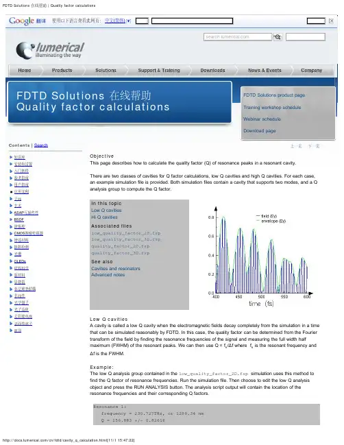
知识库安装和设置入门教程参考指南用户指南应用实例天线艺术ASAPBSDF谐振腔CMOS增益材料缺陷检测光栅OLEDs材料科学超材料显微镜多层堆叠結構非线性光学镊子光子晶体太阳能电池表面等离子波导A cavity is called a low Q cavity when the electromagnetic fields decay completely from the simulation in a timeFDTD Solutions 在线帮助Quality factor calculations FDTD Solutions product page Training workshop schedule Webinar schedule Download page)SearchResonance 2:frequency = 205.814THz, or 1456.62 nmQ = 77.498 +/- 0.226738The analysis script also creates two plots. The plot shown below to the left contains one of the field components (Hz). You can see that the fields have decayed by the end of the simulation time. The second plot shows the location and relative amplitude of the resonance peaks.Note that the initial transients of the source are neglected by setting the "start time" for the time monitors to 200fs. The "start time" for the time monitors is the time at which the monitors begin recording data. This setting can be changed in the user properties for the analysis group. Also, note that in the analysis group, it is possible to use one time monitor or an array of time monitors for the Q factor calculation. The problem with using one time monitor is that if the one monitor is placed at or near a null of the cavity mode, then due to the fact that the field intensity is very low, the Q factor can have a large uncertainty (if it is even possible to obtain a meaningful result).The low_quality_factor_3D.fsp simulation file contains a 3D version of the low Q analysis object.High Q cavitiesA cavity is considered to be a high Q cavity when the electromagnetic fields cannot completely decay from the simulation in a time that can be simulated reasonably by FDTD. In this case, we cannot determine Q from the frequency spectrum because the FWHM of each resonance in the spectrum is limited by the time of simulation,Tsim , by FWHM ~ 1/Tsim. Instead, the quality factor should be determined by the slope of the envelope of thedecaying signal using the formulawhere fRis the resonant frequency of the mode, and m is the slope of the decay in SI units.Derivation of Q factor formula:The quality factor (Q) is defined aswhere wris the resonant frequency and FWHM is the full width half max of the resonance intensity spectrum. The time domain signal of the resonance is described bywhere α is the decay constant. The fourier transform of E(t) is easy to calculate.The maximum value of |E(w)|^2 is clearly 1/α^2, at w=wr. With a little more work, we can determine that thehalf max frequencies occurs at w=wr + α and w=wr- α. Therefore, FWHM = 2α. Substituting this value intothe original Q formula and solving for α givesNow that we know how to relate α to Q, we must determine how the slope of the time signal decay is related to Q. We must take the log of the time signal to make the envelope a linear function.where m is the slope of the log of the time signal envelope. Solving for Q, we get.Example:Calculation of the Q factor for high Q cavities is complicated because•separating the decay of the envelope from the underlying sinusoidal signal is difficult since the fields are typically real-valued•if there are multiple resonant modes, they will interfere with each other in the time domain, making it hard to estimate the decay rate.By opening the edit dialog box for the Q factor analysis object located in quality_factor_3D.fsp, you can see that the analysis object solves these problems by•accurately calculating the envelope of the time-domain field signal•isolating each resonance peak in the frequency domain using a Gaussian filter, and then taking the inverse Fourier transform to calculate the time decay separately for each peak. The slope of the time decay is then used to calculate the Q factor and obtain an error estimate.In addition, note that:•the Q analysis object has setup variables that allow you to choose how many time monitors to use to calculate the Q factor. It is often a good idea to add a few point monitors at different locations to reduce the chances that a monitor is placed at a node in the mode profile of a cavity mode yielding a weak signal.•in the analysis tab, there is a parameter that can be set to choose how many resonant peaks to look for •all the field components that are available are used to calculate the Q factor•it is possible to change other parameters, such as the Gaussian filter width and resolution in the frequency domain. These parameters are set in the analysis script.•in the script, only the part of the time signal lying in 40-60% of the time signal collected is used for the slope calculation. These percentages can easily be changed. However, setting the upper limit to anything greater than 90% can lead to errors due to the fact that Fourier transforms, and inverse transforms were used when the Gaussian filter was used to isolate the peak. The Fourier transforms introduce errors to the end of the time signal due to the fact that discrete Fourier transforms assume periodicity of the signal.Next, run the simulation. When the simulation is complete, choose to edit the analysis object and press RUN ANALYSIS button. The analysis script output will contain the location of the resonance frequencies and their corresponding Q factors.Resonance 1:frequency = 178.786THz, or 1676.82 nmQ = 306.279 +/- 1.41318Resonance 2:frequency = 227.307THz, or 1318.89 nmQ = 274.874 +/- 4.50921The analysis object also produces the following plots.The time decay of the field components and their envelopes. Note The spectrum and the Gaussian filtersThe spectrum of resonances. Each resonant peak appears in a The time decay of the sum of squared Other versions of this page:Events。
FDTD Solutions资料集锦专题资料(二)
更新时间:2015-2-4
以下是小编整理的一些FDTD Solutions资料集锦,其中包括了有关FDTD
Solutions 应用算例和相关外文文献。有关文档的下载,可以到研发埠 网站的专题模块,输入相应的专题名,搜索到相应的专题便可以找umerical investigation of heat transfer in phase change
materials (PCMs).pdf The effects of metal foams on heat transfer enhancement in Phase Change Materials (PCMs) are investigated.The numerical investigation is based on the two-equation non-equilibrium heat transfer model,in which the coupled heat conduction and natural convection are considered at phase transition and liquid zones. The numerical results are validated by experimental data.
toward achieving high efficiencies in solar cells. Here we propose
a perpendicular elliptical silicon nanowire (PEE-SiNW) array for broadband light absorption in thin film silicon solar cells.
微纳光子学设计仿真工具-FDTD Solutions 专题资料集锦

Effect of subwavelength annular aperture.pdf
Fabrication and properties of metalo-dielectric photonic crystal.pdf
Educational Software for interference and optical diffraction
SMALL AREA RIGHT ANGLE BENDS.pdf
表面等离子共振技术.pdf
表面等离子体亚波长光学.pdf
李灿光催化综述.pdf
FDTD Solutions初级技术培训(视频)
更多资料:/Home.html
FDTD Solutions 8.0 - New Features(视频)
相关阅读: 纳米光学软件 FDTD Solutions
专业的微纳光子学设计分析软件
新型纳米超材料:可见光能无限穿透
上海交大发明纳米光学质谱仪检测人体癌细胞
CMOS图像传感器的发展走向
相关下载: Can information of chemical reaction propagate with plasmonic waveguide.pdf
analysis in fresenel and fraunhofer regions based on matlab guis
and the FDTD Nethos.pdf
Fabrication of Tungsten Photonic Crystals for High.pdf
FDTD Solutions_getting_started.pdf
Application of Surface Plasmon Polaritons in CMOS Digital
FDTD Solutions资料集锦专题资料(一)
如何成功完成您的Lumerical注册.pdf
算例下载区:
谐振腔相关算例:
FDTD案例-谐振腔-光学晶子.rar
FDTD案例-谐振腔-quality_factor.rar
FDTD案例-谐振腔-低质因子.rar
FDTD案例-谐振腔-型腔回音壁.rar
FDTD案例-谐振腔-PC_3D.rar
FDTD案例-谐振腔-型腔模振幅.rar
克斯普朗克研究院、麻省理工学院、美国国家标准与技术研究院、东京大学
、清华大学、北京大学和中国科学院多个研究所等,都在使用Lumerical的设 计软件软件。
FDTD参考手册
Lumerical 2014a安装手册.pdf
Lumerical Flexnet code license安装步骤(最新).pdf
FDTD Solutions资料集锦 专题(一)
更新时间:2015-2-4
以下是小编整理的一些FDTD Solutions资料集锦,其中包括了有关FDTD
Solutions FDTD参考手册、应用算例。有关文档的下载,可以到研发埠 网站的专题模块,输入相应的Байду номын сангаас题名,搜索到相应的专题便可以找学软件 FDTD Solutions
FDTD Solutions软件由加拿大Lumerical Solutions公司出品。通过向研究和 产品开发专业人士提供基于计算技术最新发展的高性能光学设计软件, Lumerical帮助光学设计者达到挑战性设计目标,满足严格的设计期限要求。 Lumerical的设计软件已在 30多个国家应用,全球科技领先厂商,如安捷伦 、ASML、博世、佳能、Harris、Northrop Grumman、奥林巴斯、飞利浦、三 星和意法半导体,以及众多卓越研究机构,如哈佛大学、加州理工学院、马
FDTD基本介绍
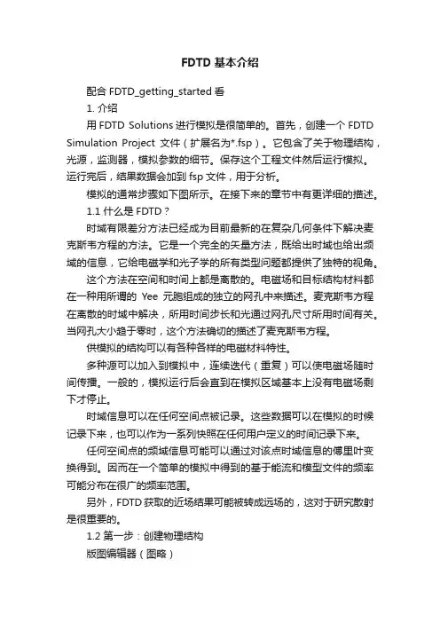
FDTD基本介绍配合FDTD_getting_started看1. 介绍用FDTD Solutions进行模拟是很简单的。
首先,创建一个FDTD Simulation Project文件(扩展名为*.fsp)。
它包含了关于物理结构,光源,监测器,模拟参数的细节。
保存这个工程文件然后运行模拟。
运行完后,结果数据会加到fsp文件,用于分析。
模拟的通常步骤如下图所示。
在接下来的章节中有更详细的描述。
1.1 什么是FDTD?时域有限差分方法已经成为目前最新的在复杂几何条件下解决麦克斯韦方程的方法。
它是一个完全的矢量方法,既给出时域也给出频域的信息,它给电磁学和光子学的所有类型问题都提供了独特的视角。
这个方法在空间和时间上都是离散的。
电磁场和目标结构材料都在一种用所谓的Yee元胞组成的独立的网孔中来描述。
麦克斯韦方程在离散的时域中解决,所用时间步长和光通过网孔尺寸所用时间有关。
当网孔大小趋于零时,这个方法确切的描述了麦克斯韦方程。
供模拟的结构可以有各种各样的电磁材料特性。
多种源可以加入到模拟中,连续迭代(重复)可以使电磁场随时间传播。
一般的,模拟运行后会直到在模拟区域基本上没有电磁场剩下才停止。
时域信息可以在任何空间点被记录。
这些数据可以在模拟的时候记录下来,也可以作为一系列快照在任何用户定义的时间记录下来。
任何空间点的频域信息可能可以通过对该点时域信息的傅里叶变换得到。
因而在一个简单的模拟中得到的基于能流和模型文件的频率可能分布在很广的频率范围。
另外,FDTD获取的近场结果可能被转成远场的,这对于研究散射是很重要的。
1.2 第一步:创建物理结构版图编辑器(图略)用Structures列表创建几何结构。
他们的特性用EDIT编辑。
工具栏,在左边。
用Aligning按钮安排对象的位置。
材料特性:可自行定义或从数据库中选择。
1.3 第二步:设置模拟区域和时间用ADD SIMULATION REGION设置:模拟区域,其大小和位置,网格精度,合适的边界条件。
FDTD Solutions资料集锦专题资料(三)
Microstructural effect on the radiative properties of YSZ thermal barrier.pdf 辐射性质YSZ热屏障对显微结构的影响 Thermal barrier coatings (TBCs) are not the pure bulk materials,
Gradient-index meta-surfaces as a bridge linking propagating waves and surface waves..pdf The arbitrary control of electromagnetic waves is a key aim of photonic research. Although, for example, the control of freely
FDTD Solutions资料集锦 专题资料(三)
更新时间:2015-2-4
以下是小编整理的一些FDTD Solutions资料集锦,其中包括了有关FDTD
Solutions 相关外文文献。有关文档的下载,可以到研发埠网站的专题 模块,输入相应的专题名,搜索到相应的专题便可以找erface temperature of liquid–solid is considered as a constant
freezing point, but majority of materials have a freezing temperature range and the freezing temperature descends with the
cell on light trapping was investigated. For various amount of
FDTD
3. The Finite-Difference Time-
Domain Method (FDTD)
The Finite-Difference Time-Domain method (FDTD) is today’s one of the most popular technique for the solution of electromagnetic problems. It has been successfully applied to an extremely wide variety of problems, such as scattering from metal objects and dielectrics, antennas, microstrip circuits, and electromagnetic absorption in the human body exposed to radiation. The main reason of the success of the FDTD method resides in the fact that the method itself is extremely simple, even for programming a three-dimensional code. The technique was first proposed by K. Yee, and then improved by others in the early 70s.
FDTD介绍
差分格式
❖ 首先,在直角坐标系中将问题空间沿三个坐标轴方向分成多 个网格单元,其中 x , y , z 分别表示在x、y、z坐标方向 的网格空间步长,用Δt表示时间步长。设 f (i,j,k)代表电场或磁 场的,某一分量在时间和空间域中的离散表达式为
f (i,j,k)= f (i x ,j y ,k z )= (i,j,k)
第二十页,编辑于星期四:七点 二十九分。
数值色散和解的稳定性
❖ 由于 FDTD 方程只是原 Maxwell 旋度方程的一种近似,在计 算中存在误差。只有离散后差分方程组的解是收敛和稳定的, 这种代替才有意义。收敛性是指当离散间隔趋于零时,差分方 程的解在空间任意一点和任意时刻都一致趋于原方程的解。稳 定性是指寻求一种离散间隔所满足的条件,在此条件下差分方 程的数值解与原方程的严格解的差为有界。
第十五页,编辑于星期四:七点 二十九分。
差分格式
❖ Yee网格如图2.2所示,主要表示的是电场和磁场在空间各节 点的排布。由图可以看出每个电场的分量周围有四个磁场分量, 相应的每个磁场分量周围也有四个电场分量。这种空间的设置 方式能够实现空间坐标的差分计算,并且考虑到电磁场在空间 互相正交、铰链的关系,也满足了Maxwell方程的积分形式,能 够很好地模拟电磁场传播过程。
❖ 随着当代半导体制作工艺的发展, 电子设备越来越趋向于小 型化和复杂化,其工作环境也日益复杂,同时电磁环境效应问题 变得也越来越重要。虽然在应用电磁数值仿真技术方面做了很 多研究, 但是实际应用的数值方法仍存有挑战性,特别是如何使 用和如何发展现有的电磁场数值技术以适应电大尺寸和多尺度 问题仿真。
第三页,编辑于星期四:七点 二十九分。
FDTD Solutions 7.0版介绍
Lumerical Solutions公司FDTD Solutions 7.0版为微纳光学设计提供优化和共形网格化技术2010/10/29/11:27来源:MarketwireMarketwire2010年10月26日不列颠哥伦比亚省温哥华消息——全球纳米光学设计软件供应商LumericalSolutions公司今天宣布,其旗舰产品FDTDSolutions7.0版已经进行了创新性升级。
升级项目包括集成参数扫描分析与优化计算、业内首个面向纳米光学设计的共形网格和一个方便复杂器件设计的扩展仿真元器件库。
Lumerical首席技术官JamesPond博士表示:“FDTDSolutions7.0延续了Lumerical的传统:在易用的电脑辅助设计环境下整合最先进的算法,为突破性创新提供得力设计工具。
FDTDSolutions7.0与非常适用的优化算法相结合,是目前最好的工业级纳米光学设计软件。
设计人员和研究人员现在可以通过评估和优化他们的最佳设计概念来迅速取得进展。
”为优化、计算速度和精确性而设计FDTDSolutions7.0能让终端用户通过其独有的共形网格技术工具,获得更高的计算效率和精度。
在数字成像和太阳能等快速发展的行业,通过采用共形网格技术而获得更高精度的仿真结果,受到越来越多的追捧。
共形网格技术是通过麦克斯韦积分方程对不同介质之间界面的复杂描述,可达到亚晶胞精度。
与其它为低频应用(在这些应用中多数金属接近完美导体)而设计的类似技术不同的是,Lumerical的技术建立在其专有的高精度多系数材料特性拟合上,能精确模拟实际光学器件设计中任意色散介质之间的界面。
加利福尼亚州帕洛阿尔托的博世研究与技术中心高级工程师InnaKozinsky博士表示:“我们使用FDTDSolutions解决薄膜太阳能电池中的光传播问题。
现实生活中的太阳能电池器件相当复杂,包含多层材料,而FDTDSolutions7.0的共形网格使我们能够优化太阳能电池活性层的吸收,而不是手工设置非常精细的网格和分析大量的仿真结果。