1 Implementation of the Convex Edge Segment
Convex_Hull

convex
not convex
Convex hulls
Preliminaries and definitions Vertices A polygon vertex is convex if its interior angle It is reflex if its interior angle > reflex convex
In a convex polygon, all the vertices are convex. In other words, any polygon with a reflex vertex is not convex.
Convex hulls
Preliminaries and definitions Convex hull, definition 2 The convex hull H(S) of a subset of points S in a plane is the set of all convex combinations of the points of S. It should be intuitively clear that a hull defined in this way can not have a “dent” (reflex vertex). Note now that S in this definition is an infinite set. The convex hull is the smallest convex set that contains S. To be more precise, it is the intersection of all convex sets that contain S.
立体信息检测苹果表面缺陷(平行的结构光)
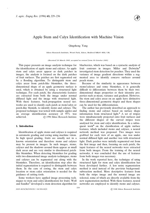
Q .Y A N G230 T he proposed system has been tested with samplea pples and the test results are presented .2.S egmentation of dark patchesD ark patches in apple images represent boths tems / c alyxes and patch-like blemishes , such asb ruises , wounds and many rots . They appear asc onnected regions of relatively small size and havev ariable shape and contrast . An example image iss hown in F ig .1 . When viewing the intensity image asa topographic relief , the patches appear as concavea reas in the grey-level surface .Therefore , they can bet reated as catchment basins in grey-level landscapes .B ased on this , a region-based segmentationa lgorithm , 5 called a flooding algorithm , has beend eveloped to segment the patches .Here , we explaint he underlying concepts of the algorithm in terms ofd igital elevation models ; the implementation detailsa re described in reference 5 .T he flooding algorithm is based on the concept ofw ater catchment basins . A catchment basin is a regiona ssociated with a minimum . To define the spatiale xtent of the region around the minimum , we considert he properties of water flowing over a topographicr elief . Water will always flow downhill until a localm inimum is reached . As more water is added ,ita ccumulates at the lowest points and gradually coverst he region surrounding the minimum , until it reaches ac ertain level at which the basin can no longer hold anym ore water and the surplus water spills over thel owest points of the basins’ rim .Thus , the basinb ecomes a lake .The corresponding elevation level ofF ig . 1 . A n example apple image with a blemish and a stema rea t he lake’s surface is called the spillover level .The s pillover level is used to delimit the spatial extent of a c atchment basin .Therefore , a catchment basin con- s ists of those points , which are connected to a m inimum and have a grey-level lower than the spillo-v er level . To detect all the dark patches ,we gradually flood the relief with water , all the catchment basins w ill be filled up and become lakes of various sizes and d epths . The lakes , which are equivalent to catchmentb asins , are the output of the flooding algorithm and r epresent the patches being detected . T he concept of a lake is extremely useful in that it h olds most of the characteristics desired in the follow-i ng classification . For instance , the surface area of a l ake is a clear indicator of the size of the detected p atch ;the average depth , i . e . the ratio of the water v olume to the lake surface area , is a measure mostly o f contrast , but contains gradient information as well . A nother obvious advantage of this presentation is that t he surface of each individual lake is always con-n ected . The segmentation result of the example image i n F ig .1 is shown in F ig .2 . The detected patches are h ighlighted with bright borders . T he algorithm has no tuning parameters , and the s egmentation output depends purely on image data . T here is little need for thresholding . It has no strong a ssumption about the contrast and shape of patches . T he sole working assumption used is that the patches a re not adjacent to the boundary of the fruit in i mages . Apart from the segmentation output ,some d escriptive parameters such as the minimum height ,c urrent volume and depth of the basins can also be c omputed as the flooding proceeds , and they are a vailable as outputs of the procedure .Once the F ig . 2 . R esults of patch segmentation for the image in Fig . 1 . D etected patches are highlighted by bright bordersA P P L E S T E M A N D C A L Y X I D E N T I F I C A T I O N W I T H M A C H I N E V I S I O N231p atches are segmented out,measurements of the c orresponding lakes can be made to extract other g eometric parameters.These parameters quantify the c haracteristics of each patch under consideration and a re ready to be used as inputs to the following c lassification step.3.T hree-dimensional shape information froms tructured lightT he surface of an apple can be divided roughly, a ccording to shape,into two basic parts,convex parts a nd concave parts.Most of the surface is convex and s ometimes nearly spherical.The concave parts are u sually in the areas around the stem and calyx.The s tem itself stands out from the middle of the concave a rea.On the other hand,blemishes,such as bruises a nd abrasions often occur on the convex surface of a f ruit.Therefore,the three-dimensional information a bout the dif f erence in surface shape can assist iden-t ification of the stem and calyx.A technique called l ight striping6i s used,in which the projected light p lanes and a camera make up an active stereo system s o that three-dimensional geometric information ab-o ut an object surface may be derived from optical t riangulation.F or fast processing,a set of evenly spaced parallel l ight stripes are projected onto the apple surfaces s imultaneously.An image with the stripes is grabbed f or each view of a fruit.This stripe image is obtained w ith the same camera as for the normal apple image w ithout the structured light.In stripe images,the s tripes on dif f erent parts of the surface have dif f erentF ig .3.A n example image with light stripes on the same apple a s shown in Fig .1. Stripes on dif f erent parts of the surfaceh ae dif f erent shapes s hapes.The stripes on convex surfaces are continuous a nd parabolic,and their curvature directions are m aintained.Stripes on nearly flat surfaces are almost p arallel.For concave surfaces around stem and calyx a reas,the appearance of stripes is complex.Stripes are n ot always parallel,can touch adjacent stripes due to s harp changes in depth,and can appear broken due to o cclusion.In the case of the continuous stripes,their c urvatures change sign when the surface changes from c onvex to concave.The stripes across stems are b roken owing to the depth discontinuity.F ig .3shows a n example image with light stripes on the same apple a s in F ig .1.T he correspondence between the shape of the s tripes and the shape of surface parts,provides the n ecessary three-dimensional information and this can b e obtained from the analysis of the dif f erent shape p atterns of curved stripes.Since stems and calyxes a ppear as patches in images,the analysis is directed to t he local area around each patch,which is first s egmented out with the flooding algorithm.Each s egmented patch in the apple image has a correspond-i ng area at the same location in the stripe image. T herefore,a rectangular window is placed around this a rea in the stripe image.The derivation of the t hree-dimensional information is thus reduced to the e xtraction of stripe patterns within each window.Note t hat in this way,the time- consuming reconstruction of t he actual three-dimensional geometric surface and t he associated calibration,as in the usual application o f light striping,are avoided.A principal parameter for describing the shape of t he stripes is curvature.On a convex surface,the s tripes are continuous and therefore have smoothly c hanging curvatures which may keep the same sign.If t he curvature of the stripes within a window varies d ramatically and changes sign,then the surface inside t he window should normally be a stem or calyx area (see discussion section for other cases).Before the c urvature is calculated,the stripe image is binarized b y a local thresholding process and then the stripes a re thinned to one pixel wide skeleton curves by a s hape preserving thinning method.7T he stripes are t hen represented by their skeleton curves,from which t heir curvatures are computed.The thinning result of F ig .3is shown in F ig .4.T he normal curvature calculation for planar digital c urves is notoriously inaccurate.Here we use a c urvature estimator for the skeleton curves.Let xϭx[s(t)]a nd yϭy[s(t)] be a skeleton curve in its p arametric form,where s is the arc length of the curve a nd is represented as a linear function of parameter t,sϭs(t).Let (s) represent the tangent angle of the c urve at s.The point curvature k o f the curve isQ.Y A N G 232F ig .4.T he thinning result of Fig .3d efined as the instantaneous rate of change of w ith r espect to arc length sk(s)ϭd(s)/d s(1) w here[s(t)]ϭt anϪ1y(t)x(t)(2)T o reduce the noise caused by taking the second-order d erivatives in the usual calculation of curvature,we u se the following practical method to approximate the c urvature.Let the increment ds be a small constant, t hen the dif f erenced(t)Ϸ(tϩ1)Ϫ(t)(3) c ontains curvature information.We,therefore,define t he dif f erence as an estimator of the point curvaturekϭ(tϩ1)Ϫ(t)(4) T o reliably calculate i n Eqn (4),we smooth the c urve,xϭx(t)and yϭy(t),with a Gaussian kernel g(t,)o f standard deviation .The smoothed curve, X(t,)a nd Y(t),is expressed asX(t,)ϭx(t)ءg(t,)ϭ͵3Ϫ3x(u)142πeϪ(tϪu)2/22d u(5) Y(t,)ϭy(t)ءg(t,)ϭ͵3Ϫ3y(u)142πeϪ(tϪu)2/22d u(6)w here u i s a dummy integral variable and ءi s the s tandard symbol for convolution.Their first deriva-t ives are expressed asX(t,)ϭx(t)ءѨg(t,)Ѩtϭ͵3Ϫ3x(u)Ϫt342πeϪ(tϪu)2/22d u(7) Y(t,)ϭy(t)ءѨg(t,)Ѩtϭ͵3Ϫ3y(u)Ϫt342πeϪ(tϪu)2/22d u(8) S o (t) in Eqn (4) is computed as(t)ϭt anϪ1Y(t)X(t)(9)N ote that whilst the angle function (t) in Eqn (9) is m ultiple-valued,under practical constraints on con-t inuity of the derivative,it is uniquely defined.4.F eature selectionI n this study,the features are intuitively determined t o provide reasonable coverage of the feature space. O nce a small patch is segmented out from an apple i mage,some features of the patch are already avail-a ble,which include the lowest grey-level I l,the highest g rey-level I h,the area A,the boundary length C p a nd t he water volume V o f the lake representing the patch. O ther features,including curvature,are extracted f rom both the apple image and the stripe image.F or the curves within a focusing window,some s tatistics of curvature are computed.These are ave-r age positive and negative curvatures,K p a nd K n,the a verage absolute curvature ͉K͉,and the frequencies of p oints with positive,negative and zero curvature,F p, F n a nd F z,respectively.These statistics describe the c oarse distribution of the curvature.A n important descriptor for the shape patterns of s tripes is the similarity between the shapes of curves. T he stripes crossing a convex surface have greater s imilarity (i.e.are more parallel),than those crossing s tem and calyx areas.The similarity can be measured b y the correlation of curvature between curves.Ther-e fore the average correlation coef ficient R c i s selected. T he length of the analysed curves within a window is a g ood indicator of their continuity,which is strongly r elated to blemishes on convex surfaces.Hence,the a verage curve length L m i s included as a feature.On t he other hand,the relative number of short curveA P P L E S T E M A N D C A L Y X I D E N T I F I C A T I O N W I T H M A C H I N E V I S I O N233s egments within a window is a clue to the irregularity o f the stripes.The short curve segments refer to the s mall curves that are not long enough for computing t heir smoothed curvature.They usually occur on thec oncave stem and calyx areas where stripes ared iscontinuous owing to sudden change in depth.So, t he relative number of short curve segments S s i s c omputed.I n apple images,when a standing stem appears as a p rotrusion or the small spikes of a calyx appear on theb oundary of a patch,the boundary is likely to be morec omplex than that of a blemish.Hence,the compact-n ess P o f the patch is selected,which is defined as the r atio of the squared perimeter C p2to the area A,i.e. PϭC p2/A.The perimeter C p i s simply the count of p ixels on the patch boundary.Two shape measure-m ents of the water volume of the lake are also s elected.These are the average depth h a o f the v olume,defined as V/A,and the ‘‘conical’’ angle ␣o f t he volume,which is defined as the average radius d o f t he boundary to the lake’s centre divided by the m aximum depth of the water,i.e.d/(I hϪI l).To c ompute this latter measure,the geometric centroid of t he lake surface is found by the first moment method. T o complete,the primary intensity properties,mean I m a nd variance Io f the grey-level in a patch,are i ncluded.A ltogether,eighteen features are extracted for each p atch and are summarized as follows.F rom the stripe image :K p a verage positive curva-t ure,K n a verage negative curvature,͉K͉a verage a bsolute curvature,F p f requency of points with posi-t ive curvature,F n f requency of points with negative c urvature,F z f requency of points with zero curvature, R c a verage correlation coef ficient of curvature bet-w een curves,L m a verage curve length,S s p ercentage o f short curve segments,F rom the apple image :I m a verage grey level inten-s ity,Iv ariance of grey level intensity,I l l owest grey l evel of the patch,I h h ighest grey level of the patch,A a rea of the patch,P c ompactness of the area,V w ater v olume of the lake,␣c onical angle of the volume,h a a verage depth of the volume.A s can be seen,these features are not independent.B ut in this study,we do not address the issue of s alient feature selection.Since the dependencies are n ot easily modelled and the features are not dif ficult t o compute,we retain all the features for the following c lassification.5.C lassification of patches with neural networksO nce the feature vector is extracted for each patch, s tems and calyxes can be identified by feeding the f eatures into a classifier and classifying the patch as e ither blemish or stem/c alyx,which are two possible o utput classes.The input feature data to the classifier p ossess some nonlinear relations to their correspond-i ng surface types.F ig .5a s hows a set of average p ositive and negative curvature data for two types of p atches.F ig .5b s hows mean intensity and variance. T he data are from the first group of samples (Training1).It can be seen from these figures that the twoc lusters representing the two classes are not linearly s eparable for these variables.A non-linear classifier is r equired.I n this work, a multi-layer feedforward neural n etwork was constructed for the classification.Three d if f erent network configurations,(18 :10:2),(18:27:2) a nd (18:10:6:2) were tested.No attempt was made to find an optimal network configuration and it might be p ossible to reduce the complexity of the net.The n etwork was fully connected.The number of nodes in t he input layer was the same as the number of input–0·1–0·2–0·3–0·4Averagenegativecurvature0·000·050·100·150·200·25Average positive curvature(a)(b)0·70·60·50·40·30·20·10·00·00·20·40·60·81·0Average grey-levelVarianceofgrey-levelintensityF ig .5.D istribution of two classes in feature sub -s pace .(a) S cattergram of ae rage positie cura ture e rsus ae rage n egatie cura ture for blemish and stem/c alyx ;(b) s cattergram of mean grey -l ee l intensity e rsus a riance of g rey -l ee l intensity for the two types of patches .ᮀ,blemishes ;ϫ,stalks/c alyxesQ.Y A N G 234f eatures (18).The output layer of the neural network w as composed of two nodes to correspond to the two o utput classes.The hidden layer contained ten nodes i n the first configuration,27 in the second.The third c onfiguration had two hidden layers with ten and six n odes respectively.The nodes in the output layer and h idden layer(s) had a non-linear transfer function of s igmoidal shape.The network was trained with a m odified back-propagation learning algorithm.8T he a lgorithm accelerated the learning by changing the t wo coef ficients used in the conventional back-p ropagation algorithm,learning rate and momentum f actor.D uring the training,the weights of the network w ere updated after each pass through all the training s amples.The desired outputs for each nodes in the o utput layer were arranged in an on –o f f manner,i.e. (1,0) represented blemish and (0,1) represents s tem/c alyx.The convergence of the learning was j udged by two conditions :whether the mean squared e rror for all training samples was smaller than a c riterion and whether the output errors for each t raining sample were all smaller than another c riterion.6.E xperimental resultsT he proposed techniques were tested with Golden D elicious and Granny Smith apples obtained from two p ackhouses in southern France.The apples were g raded in terms of surface defects by skilful inspec-t ors.Table 1 lists the number of sample fruits from e ach variety and grade.T he experimental arrangement for image acquisi-t ion comprised a CCD monochromatic camera (Pana-s onic,model WV-CD20),a projector for structured l ighting,and a light chamber for dif f use lighting.The a ngle between the optical axes of the camera and the p rojector was 20Њ.The light stripes were formed by p rojecting light through an optical grid of thin tran-s parent lines.The camera was mounted above the topT able 1S ample applesG radeA pple a riety E xtra I I I I II T otalG oldenD elicious1214462698G ranny Smith810382480o f the lighting chamber.Apples were placed in the m iddle of the field of view.The orientation of the s ample fruits was chosen in a random manner.For t he blemish-free fruits from the Extra grade,the s tems/c alyxes were made visible to the camera.The b ackground of the viewing field was black.The video s ignal of the camera was sent to a transputer-based f rame grabber,where it was digitized into video m emory with 512ϫ512 spatial resolution and 8 bit g rey-level resolution.All images were stored and s hown in this paper in the size of 256ϫ256 pixels.T wo images were acquired for each view of an a pple.One was under dif f use illumination,another w as under structured light.A few apples had more t han one blemish on dif f erent sides of the fruit,hence m ultiple pairs of images were recorded for each of t hese apples.The flooding algorithm was applied to s egment out dark patches from apple images.For each s egmented patch,the selected 18 features as described i n the previous section were extracted from both i mages.The type of the patch,i.e.blemish or s tem/c alyx,was recorded together with the features, t o form a labelled sample.As shown in Table 2,a t otal of 274 samples were collected and arranged in f our sets.Two of them were training samples,the o ther two were used to test the performance of the t rained neural network classifiers.There were no t raining samples included in the test sample sets.The b lemish category included bruise,russet,scab,wound, i nsect bite,sun-burn and rot.T he extracted features had very dif f erent ranges of v alues,so to input them to the neural networks,the f eature values were normalized to the range of [0,1и0].The neural networks were implemented on a t ransputer system.In all the trainings the initial l earning rate and momentum factor were fixed at 0и1 a nd 0и5 but the training algorithm employed was not v ery sensitive to these initial values.The weights of t he networks were all initialized with random numbers i n the range of [0,1и0].The convergence criteria of the n eural network during learning were set to be less t han 0и001 for mean squared error and 0и01 for a bsolute output error of each training sample.These v alues are relatively small and were chosen to allow a ccurate learning with little loss of the generalizationc apability of the networks.All trainings with somed if f erent sets of initial weights converged rapidly, w ithin about 100 to 800 iterations.I n the performance evaluation for the trained neu-r al networks,a range of 0и3 was set in the interpreta-t ion of classification outputs,instead of the crisp o n-of f outputs (1,0) and (0,1).That is,a node in the o utput layer was regarded to be ‘‘on’’ if its output v alue was larger than 0и7,‘‘of f’’ if less than 0и3,A P P L E S T E M A N D C A L Y X I D E N T I F I C A T I O N W I T H M A C H I N E V I S I O N235T able 2D if f erent types of samplesA pple a riety S amplesB lemish S tem/c alyx S ubtotal T otalG olden Delicious T raining 1473784T est 1442569274G ranny Smith T raining 2511566T est 2411455‘‘unknown’’ if between 0и3 and 0и7.The pattern p resented at the input layer was classified to belong to t he category that the ‘‘on’’ node represented.Thus,if t he outputs of the two nodes in the output layer were i n the range (1и0–0и7,0и3–0и0),the input patch was a ccordingly classified into the blemish category,and if t hey were in (0и0–0и3,0и7–1и0),the stem/c alyx c ategory.If both nodes were either ‘‘on’’ or ‘‘of f’’ and i f a node had ‘‘unknown’’ output,the input patch was c lassified into the unknown category.The selection of r ange 0и3 was conservative and imposed a strict r equirement for the networks.The range could be r elaxed to a slightly greater value.T he classification results are listed in Tables 3 and 4. T able 3 shows the classification accuracy in each test. T he accuracy was computed by dividing the number of c orrectly classified samples by the number of samples i n the test group.Table 4 shows the number of c lassification errors.Error I r efers to the misclassifica-t ion of stem/c alyx as blemish,Error I I i s vice versa,a nd Error I II r efers to the case in which either ab lemish or stem/c alyx input patch is classified into the u nknown category.It can be seen from Table 3 that t he classification accuracy of the three network con-figurations is about the same.As shown in Table 4, t he number of errors in the unknown category is s lightly reduced in the case of Test 1 with the network c onfiguration (18:10:6:2) and the case of Test 2 with t he network configuration (18:27:2).Since the first c onfiguration with 10 nodes in the hidden layer has m uch less complexity and its performance is accep-t able,it is to be preferred.The same number of errors i n Errors I a nd I I f or dif f erent configurations indicatesT able 3C lassification accuracy of the trained neural networksC lassification accuracy (%)N etworkc onfiguration T est 1T est 218:10:295и7 94и518:27:295и7 96и418:10:6:297и1 94и5T able 4C lassification errors of the trained neural networksN umber of errors S ampleg roup E rror type(18:10:2)(18:27:2)(18:10:6:2)T est 1I 0 0 0I I 1 1 1I II 2 2 1T est 2I 1 1 1I I 1 1 1I II 1 0 1t hat one or two specific pattern samples have feature v alues in the range of the ones for the other class.In t hese cases,persistent errors would occur.On the w hole,good classification accuracies have been a chieved.7.D iscussionT he technique developed in this paper is based on a n assumption that blemishes only occur on convex or flat surfaces of apples and therefore the light stripe p atterns on them reflects the type of the surface.It c an cope with the cases in which the blemished s urfaces are slightly indented.But,if the surface of a b lemish has a significantly concave shape as in cases of s evere mechanical damage,or a blemish occurs on the c oncave areas around stem or calyx,the shapes of the s tripes on the blemish will be similar to those on s tem/c alyx areas and the system will fail.Another l imitation is that if a dark patch occurs adjacent to the b oundary of a fruit in a view,the segmentation p rocess will not output it and no subsequent classifica-t ion will be made.However,in practical implementa-t ion,multiple views of a fruit are expected,so there is a good chance that the patch will not be adjacent to t he boundary of the fruit in one of the views.A n advantage of the technique is that,since onlyQ.Y A N G 236q ualitative features of stripe patterns are required, t here is no need for conventional three-dimensional s urface fitting and the calibration for the triangulation o f the structured lighting system is eliminated.This w as deliberately avoided because the complex and u npredictable stripe patterns,especially those caused b y out-standing stems,may present dif ficulties to those fitting techniques.T he technique has potential for high speed im-p lementation because of its simplicity.The necessary t hree-dimensional information is reduced to simple c onvexity or concavity,which is represented by the s hape pattern of the stripes.All segmented patches a nd all stripes on each patch can be analysed in p arallel.In the experimental arrangement,the two i mages are grabbed in sequence.If the wavelength of t he structured light is chosen in the appropriate s pectral range,the two images can be grabbed simul-t aneously by two sensors.9I t is also worth pointing out t hat the technique has the potential to be used for o ther fruits.8.ConclusionA n image analysis technique for the identification of a pple stems and calyxes has been developed.Struc-t ured light is used to provide the necessary three-d imensional shape information of apple geometric s urfaces.The analysis is focused on dark patches of f ruit surfaces,which are first segmented out by a flooding algorithm.For each patch,the qualitative f eatures of the stripe pattern are extracted from the s tripe image and the two-dimensional intensity pro-p erties are extracted from the apple image under n ormal dif f used light.When the three-dimensional a nd two-dimensional information is fused with a m ulti-layer feedforward neural network,the segmen-t ed patches are classified as stem/c alyx or blemish.T he proposed technique was tested with samplea pples and an average identification accuracy of 95%w as achieved.This result demonstrates that the system c an ef f ectively identify stems and calyxes which ares urrounded by concave surfaces,and distinguish them f rom discoloured blemishes which occur on convex or flat surfaces.A cknowledgementT his work was partly funded by the EC (CAMAR : 8001-CT91-0206).The author would like to thank P rof.A.K.Thompson at Cranfield University and Dr R.D.Tillett for valuable discussion.R eferences1W olfe R R ;Sandler W E A n algorithm for stem detection u sing digital image analysis.Transactions of the ASAE 1985,28 :641 –6442M iller B K ;Delwiche M J P each defect detection with m achine vision.ASAE Paper 89 –60193Y ang Q F inding stem and calyx of apples using structured l puters and Electronics in Agriculture 1993,8:31 –424Y ang Q C lassification of apple surface features using m achine vision and neural puters andE lectronics in Agriculture 1993,9:1–125Y ang Q A n approach to apple surface feature detectionb y machine puters and Electronics in Agri-c ulture 1994,11 :249 –2646B allard D H ;Brown C M C omputer vision,EnglewoodC lif f s,Prentice-Hall,1982,pp.52 –547G onzalez R C ;Woods R E D igital image processing,A ddison-Wesley Publishing Company,1992,pp.492 –4948C han L W ;Fallside F A n adaptive training algorithm forb ack propagation puter Speech and Lan-g uage 1987,2:205 –2189C rowe T ;Delwiche M R eal-time defect detection in fruit.I nternational Conference on Agricultural Engineering(AgEng’94),Milano,Italy,29 August –1st September 1994,Report No.94-G-027。
Delaunay三角剖分

2.没有相交边。(边和边没有交叉点)
3.平面图中所有的面都是三角面.且所有三介面的合集堆散点集V的凸包。
1.2 Delaunay
在实际中运用的鼓多的三角別分是Delaunay三角剖分.它绘一种待殊的三角剖分。先从Delaunay边说起:
【定义】Delaunay边:假设E中的一条边e(两个端点为a,b)> e若满足下列条件.则称Z为Delaunay边:存在一个閲
丄・CvPoint2D32f fp;//This is our point holder//;.^我心点的f•} fIRS)
2・for(i = 0; i < as_many_points_as_you_want; i++ ) {
3・//However you want to set points〃如果我们的点集不足32位的.在这里我们将其转为CvPoint2D32于・如下两种方法.
第//
5.fp=your_32f_point_list[i];
6.cvSubdiv0elaunay2DInsert( subdiv, fp )j
7・}
转换为
1)
2)
肖可以通过输入点(散点集)得到
1.cvCalcSubdivVoronoi2D( subdiv);//Fill out Voronoi data in subdiv〃在subdiv充Vornoi的数州
1.
以下是Delaunay剖分所具备的优异特性:
1x最接近:以掖接近的三点形成三角形.且各线段《三角行的边〉皆不相交。
2.唯一性:不论从区域何处开始构建.最终都将得到一致的结果。
3.眾优性:任惫两个相邻三角形构成的凸四边形的对角线如何可以互换的话.那么两个三角形六个内角屮最小角度不 会变化,
阿尔伦-布拉德利 Stratix 5700 工业 managed Ethernet 交换机说明书

Stratix 5700Industrial Managed Ethernet SwitchThe wide deployment of EtherNet/IP™ in industrial automation means that there is a growing demand to manage the network properly.Integtrating new machine-level networks into an existing plant network requires convergence.With more devices connected on the same Ethernet network than ever before, an industrial managed switch can help you simplify your network infrastructure. Adding a managed switch to your network architecture can also help make the process of adding new machines easier. The Allen-Bradley® Stratix 5700™ is a compact, scalable Layer 2 managed switch with embedded Cisco technology for use in applications with small isolated, to complex networks. With integration into Studio 5000 Automation Engineering and Design Environment™, you canleverage FactoryTalk® View faceplates and Add-on Profiles for simplified configuration and monitoring.By choosing a switch co-developed by Rockwell Automation and Cisco, your Operations Technology (OT) and Information Technology (IT) professionals leverage tools and technology that are familiar to them. This collaboration can also help to reduce configuration time and cost.Features and Benefits:Advanced Networking Features• Integrated Device Level Ring (DLR) connectivity helps optimize the network architecture and provide consolidated network diagnostics • Integrated Network Address Translation (NAT) provides 1:1 IP address mapping helping to reduce commissioning time • Power over Ethernet (PoE) versions provide power to devices over Ethernet minimizing cabling • Security features, including access control lists, help ensure that only authorized devices, users and traffic can access the network • Secure Digital (SD) card provides simplified device replacementOptimized integration:• Studio 5000® Add-on Profiles (AOPs) enable premier integration into the Rockwell Automation Integrated Architecture® system • Predefined Logix tags for monitoring and port control • FactoryTalk® View faceplates enable status monitoring and alarming • Built-in Cisco® Internet Operating System (IOS) helps provide secure integration with enterprise networkDesigned and Developed for EtherNet/IP Automation ApplicationsNetwork Address TranslationMachine integration onto a plant network architecture can be difficult as machine builder IP-address assignments rarely match the addresses of the end-user network. Also, network IP addresses are often unknown until the machine is being installed. The Stratix 5700 with Network Address Translation (NAT) is a Layer 2 implementation that provides “wire speed” 1:1 translations ideal for automation applications where performance is critical.NAT allows for:• Simplified integration of IP-addressmapping from a set of local,machine-level IP addresses to theend user’s broader plant network• OEMs to deliver standard machinesto end users without programmingunique IP addresses• End users to more simply integratethe machines into the larger network192.168.1.4192.168.1.4MACHINE 1MACHINE 2Private Network Private NetworkSwitch Reference ChartAllen-Bradley Stratix 5700 Industrial Ethernet SwitchSwitch Selection TableFE - Fast Ethernet GE - Gigabit EthernetPublication ENET-PP005F-EN-E – April 2016Copyright ©2016 Rockwell Automation, Inc. All Rights Reserved. Printed in USA.Supersedes Publication ENET-PP005E-EN-E – March 2015EtherNet/IP is a trademark of the ODVA.Cisco is a trademark of Cisco Systems, Inc.Allen-Bradley, CompactLogix, Factory Talk, Integrated Architecture, Kinetix, LISTEN. THINK. SOLVE., Powerflex, Rockwell Automation, Rockwell Software, Stratix 5700, Studio 5000, Studio 5000 Automation Engineering and Design Environment are trademarks of Rockwell Automation, Inc.Glossary of TermsAccess Control Lists allow you to filter network traffic. This can be used to selectively block types of traffic to provide traffic flow control or provide a basic level of security for accessing your network.CIP port control and fault detection allows for port access based on Logix controller program or controller mode (idle/fault). Allows secure access to the network based on machine conditions.CIP SYNC (IEEE1588) is the ODVAimplementation of the IEEE 1588 precision time protocol. This protocol allows very high precision clock synchronization across automation devices. CIP SYNC is an enabling technology for time-critical automation tasks such as accurate alarming for post-event diagnostics, precision motion and high precision first fault detection or sequence of events.Device Level Ring (DLR) allows direct connectivity to a resilient ring network at the device level.DHCP per port allows you to assign a specific IP address to each port, confirming that the device attached to a given port will get the same IP address. This feature allows for device replacement without having to manually configure IP addresses.Encryption provides network security by encrypting administrator traffic during Telnet and SNMP sessions.EtherChannel is a port trunking technology. EtherChannel allows grouping several physical Ethernet ports to create one logical Ethernet port. Should a link fail, the EtherChannel technology will automatically redistribute traffic across the remaining links.Ethernet/IP (CIP) interface enables premier integration to the Integrated Architecture with Studio 5000 AOP , Logix tags and View Faceplates.FlexLinks provides resiliency with a quick recovery time and load balancing on a redundant star network.IGMP Snooping (Internet Group Management Protocol) constrains the flooding of multicast traffic by dynamically configuring switch ports so that multicast traffic is forwarded only to ports associated with a particular IP multicast group.* Separate SW IOS requiredKey Software FeaturesMAC ID Port Security checks the MAC ID of devices connected to the switch to determine if it is authorized. If not the device is blocked and the controller receives a warning message. This provides a method to block unauthorized access to the network.Network Address Translation (NAT) provides 1:1 translations of IP addresses from one subnet to another. Can be used to integrate machines into an existing network architecture.Port Thresholds(Storm control & Traffic Shaping)allows you to set both incoming and outgoing traffic limits. If a threshold is exceeded alarms can be set in the Logix controller to alert an operator. Power over Ethernet (PoE) provides electrical power along with data on a single Ethernet cable to end devices.QoS – Quality of Service (QoS) is the ability to provide different priority to different applications, users, or data flows, to help provide a higher level of determinism on your network.REP (Resilient Ethernet Protocol) – A ring protocol that allows switches to be connected in a ring, ring segment or nested ring segments. REP provides network resiliency across switches with a rapid recovery time ideal for industrial automation applications.Smartports provide a set of configurations to optimize port settings for common devices like automation devices, switches, routers, PCs and wireless devices. Smartports can also be customized for specific needs.SNMP Simple Network Management Protocol (SNMP) is a management protocol typically used by IT to help monitor and configure network-attached devices.Static and InterVLAN Routing bridges the gap between layer 2 and layer 3 routing providing limited static and connected routes across VLANs.STP/RSTP/MST Spanning Tree Protocol, is a feature that provides a resilient path between switches. Used for applications that requires a fault tolerant network.VLANs with Trunking is a feature that allows you to group devices with a common set of requirements into network segments. VLANs can be used to provide scalability, security and management to your network.802.1x Security is an IEEE standard for access control and authentication. It can be used to track access to network resources and helps secure the network infrastructure.。
convex and quasi convex
separable
function.
• Why does Theorem 5 require that each φi be strictly concave to ensure that f is strictly concave, while Theorem 4 requires only one fi be strictly concave to ensure that f is is strictly concave?
i=1
i=1
This establishes that f is concave. If some fi is strictly concave and αi > 0, then the inequality is strict.
Since a constant function is concave, Theorem 4 implies:
V31.0006 Mathematics for Economists
New York University Department of Economics
C. Wilson September 15, 2011
Concave and Quasi-Concave Functions
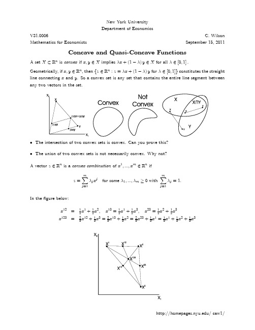
A set X ⊂ Rn is convex if x, y ∈ X implies λx + (1 − λ) y ∈ X for all λ ∈ [0, 1] . Geometrically, if x, y ∈ Rn, then {z ∈ Rn : z = λx + (1 − λ) y for λ ∈ [0, 1]} constitutes the straight line connecting x and y. So a convex set is any set that contains the entire line segment between any two vectors in the set.
模具专业英语术语
模具专业英语术语模具工程常用词汇die 模具die shoe 模座figure file, chart file图档cutting die, blanking die冲模progressive die, follow (-on)die 连续模compound die复合模punched hole冲孔 panel board镶块to cutedges=side cut=side scrap切边to bending折弯to pull, to stretch拉伸Line streching, line pulling线拉伸engraving, to engrave刻印upsiding down edges翻边to stake铆合design modification设计变化 die block模块folded block折弯块sliding block滑块location pin定位销lifting pin顶料销die plate, front board范本padding block垫块stepping bar垫条upper die base上模lower die base下模座upper supporting blank上承板upper padding plate blank上垫板spare dies模具备品spring 弹簧 bolt螺栓plate电镀mold成型material for engineering mold testing工程试模材料not included in physical inventory不列入盘点incoming material to be inspected进货待验PCE assembly production schedule sheet PCE组装厂生产排配表model机钟work order工令revision版次production control confirmation生产确认checked by初审approved by核准stock age analysis sheet 库存货龄分析表on-hand inventory现有库存available material良品可使用obsolete material良品已呆滞to be inspected or reworked 待验或重工cause description缘故说明part number/ P/N 料号item/group/class类别prepared by制year-end physical inventory difference analysis sheet 年终盘点差异分析表physical inventory盘点数量physical count quantity账面数量difference quantity差异good product/accepted goods/ accepted parts/good parts 良品defective product/non-good parts不良品disposed goods处理品on way location在途仓oversea location海外仓spare parts physical inventory list 备品盘点清单spare molds location模具备品仓skid/pallet栈板tox machine自铆机wire EDM线割 EDM放电机coil stock卷料sheet stock片料tolerance工差score=groove压线cam block滑块pilot导正筒trim剪外边pierce剪内边drag form压锻差pocket for the punch head挂钩槽slug hole废料孔feature die公母模expansion dwg展开图radius半径shim(wedge)楔子torch-flame cut火焰切割set screw止付螺丝form block折刀stop pin定位销round pierce punch=die button圆冲子shape punch=die insert异形子stock locater block定位块under cut=scrap chopper清角active plate活动板baffle plate挡块cover plate盖板male die公模female die母模groove punch压线冲子air-cushion eject-rod气垫顶杆spring-box eject-plate弹簧箱顶板bushing block衬套insert 入块capability能力parameter参数 factor系数phosphate皮膜化成viscosity涂料粘度alkalidipping脱脂main manifold主集流脉bezel斜视规blanking穿落模dejecting顶固模demagnetization去磁;消磁high-speed transmission高速传递heat dissipation热传rack上料degrease脱脂rinse水洗alkaline etch龄咬 desmut剥黑膜 D.I. rinse纯水次 Chromate铬酸处理 Anodize阳性处理 seal封孔 revision 版次 part number/P/N料号 good products良品 scraped products报放心品 defective products不良品 finished products成品 disposed products处理品 barcode条形码 flow chart流程窗体 assembly组装 stamping冲压 molding成型 spare parts=buffer备品 coordinate坐标 dismantle the die折模 auxiliary fuction 辅助功能 poly-line多义线 heater band 加热片 thermocouple热电偶 sand blasting喷沙 grit 砂砾 derusting machine除锈机 degate打浇口 dryer烘干机 induction感应 induction light感应光 response=reaction=interaction感应 ram连杆 edge finder巡边器 concave凸 convex凹 short射料不足 nick缺口 speck瑕疵 shine亮班 splay 银纹 gas mark焦痕 delamination起鳞 cold slug冷块 blush 导色 gouge沟槽;凿槽 satin texture段面咬花 witness line证示线 patent专利 grit沙砾 granule=peuet=grain细粒 grit maker抽粒机cushion缓冲 magnalium镁铝合金 magnesium镁金 metal plate钣金 lathe车 mill锉 plane刨 grind磨 drill铝 boring镗 blinster气泡 fillet镶;嵌边 through-hole form通孔形式 voller pin formality滚针形式 cam driver铡楔 shank 摸柄 crank shaft曲柄 augular offset角度偏差 velocity速度 production tempo生产进度现状 torque扭矩 spline=the multiple keys花键quenching淬火 tempering 回火annealing退火 carbonization碳化 alloy合金 tungsten high speed steel钨高速的 moly high speed steel钼高速的 organic solvent有机溶剂 bracket小磁导 liaison联络单 volatile挥发性resistance 电阻 ion离子 titrator滴定仪 beacon警示灯 coolant冷却液 crusher破裂机模具工程类 plain die简易模 pierce die 冲孔模 forming die成型模 progressive die连续模 gang dies复合模 shearing die剪边模 riveting die铆合模 pierce 冲孔 forming成型(抽凸,冲凸) draw hole抽孔 bending折弯 trim切边 emboss凸点dome凸圆 semi-shearing半剪 stamp mark冲记号 deburr or coin压毛边 punch riveting冲压铆合 side stretch侧冲压平 reel stretch卷圆压平 groove压线 blanking下料 stamp letter冲字(料号) shearing剪断 tick-mark nearside正面压印 tick-mark farside反面压印冲压名称类 extension dwg展开图 procedure dwg工程图 die structure dwg模具结构图 material材质 material thickness料片厚度press specification冲床规格 die height range适用模高 die height闭模高度 burr毛边 gap间隙 punch wt.上模重量五金零件类inner guiding post内导柱 inner hexagon screw内六角螺钉 dowel pin固定销coil spring弹簧 lifter pin顶料销 eq-heightsleeves=spool等高套筒 pin销 lifter guide pin浮升导料销 guide pin导正销wire spring圆线弹簧 outer guiding post 外导柱 stop screw止付螺丝 located pin定位销 outer bush 外导套范本类top plate上托板〔顶板〕 top block上垫脚 punch set上模座 punch pad上垫板 punch holder上夹板stripper pad脱料背板up stripper上脱料板 male die公模(凸模) feature die公母模 female die母模(凹模) upper plate上模板lower plate下模板 die pad下垫板 die holder下夹板 die set下模座 bottom block下垫脚 bottom plate下托板(底板) stripping plate内外打(脱料板)outer stripper外脱料板 inner stripper内脱料板 lower stripper下脱料板零件类 punch冲头 insert入块(嵌入件) deburring punch压毛边冲子 groove punch压线冲子 stamped punch字模冲子 round punch圆冲子 special shape punch异形冲子 bending block折刀 roller滚轴 baffle plate挡块 located block定位块 supporting block for location 定位支承块 air cushion plate气垫板 air-cushion eject-rod气垫顶杆 trimming punch切边冲子 stiffening rib punch一、 = stinger 加强筋冲子 ribbon punch压筋冲子 reel-stretch punch卷圆压平冲子 guide plate定位板 sliding block滑块 sliding dowel block滑块固定块 active plate活动板 lower sliding plate下滑块板 upper holder block上压块 upper mid plate上中间板 spring box弹簧箱 spring-box eject-rod弹簧箱顶杆 spring-box eject-plate弹簧箱顶板 bushing bolck衬套 cover plate盖板guide pad导料块塑件&模具相关英文compre sion molding压缩成型 flash mold溢流式模具 plsitive mold挤压式模具split mold分割式模具 cavity型控母模 core模心公模 taper锥拔 leather cloak仿皮革 shiver饰纹 flow mark流痕 welding mark溶合痕 post screw insert螺纹套筒埋值self tapping screw自攻螺丝 striper plate脱料板piston活塞 cylinder汽缸套 chip细碎物 handle mold掌上型模具〔移转成型用模具〕 encapsulation molding低压封装成型〔射出成型用模具〕two plate两极式〔模具〕 well type蓄料井 insulated runner 绝缘浇道方式 hot runner热浇道 runner plat浇道模块 valve gate阀门浇口 band heater环带状的电热器 spindle阀针 spear head刨尖头 slag well冷料井 cold slag冷料渣 air vent排气道 welding line熔合痕 eject pin顶出针 knock pin顶出销 return pin回位销反顶针 sleave套筒 stripper plate脱料板 insert core放置入子runner stripper plate浇道脱料板 guide pin导销 eject rod (bar)〔成型机〕顶业捧 subzero深冷处理three plate三极式模具runner system浇道系统 stress crack应力电裂 orientation 定向 sprue gate射料浇口,直浇口 nozzle射嘴 sprue lock pin料头钩销(拉料杆) slag well冷料井 side gate侧浇口 edge gate侧缘浇口 tab gate搭接浇口 film gate薄膜浇口 flash gate闸门浇口slit gate缝隙浇口 fan gate扇形浇口 dish gate因盘形浇口 diaphragm gate隔膜浇口 ring gate环形浇口 subarine gate潜入式浇口tunnel gate隧道式浇口 pin gate针点浇口 Runner less无浇道 (sprue less)无射料管方式 long nozzle延长喷嘴方式 sprue浇口;溶渣各种模具常用成形方式 accurate die casting 周密压铸 powder forming 粉末成形 calendaring molding 压延成形 powder metal forging 粉末锻造cold chamber die casting 冷式压铸precision forging 周密锻造cold forging 冷锻press forging 冲锻compacting molding 粉末压出成形rocking die forging 摇动锻造compound molding 复合成形rotary forging 回转锻造compression molding 压缩成形rotational molding 离心成形dip mold 浸渍成形rubber molding 橡胶成形encapsulation molding 注入成形sand mold casting 砂模铸造extrusion molding 挤出成形shell casting 壳模铸造foam forming 泡沫成形sinter forging 烧结锻造forging roll 轧锻six sides forging 六面锻造gravity casting 重力铸造slush molding 凝塑成形hollow(blow) molding 中空(吹出)成形squeeze casting 高压铸造hot chamber die casting 热室压铸swaging 挤锻hot forging 热锻transfer molding 转送成形injection molding 射出成形warm forging 温锻investment casting 周密铸造matched die method 对模成形法 laminating method 被覆淋膜成形low pressure casting 低压铸造lost wax casting 脱蜡铸造matched mould thermal forming 对模热成形模各式模具分类用语bismuth mold 铋铸模landed plunger mold 有肩柱塞式模具burnishing die 挤光模landed positive mold 有肩全压式模具button die 镶入式圆形凹模loading shoe mold 料套式模具center-gated mold 中心浇口式模具loose detail mold 活零件模具chill mold 冷硬用铸模loose mold 活动式模具clod hobbing 冷挤压制模louvering die 百叶窗冲切模composite dies 复合模具manifold die 分歧管模具counter punch 反凸模modular mold 组合式模具double stack mold 双层模具multi-cavity mold 多模穴模具electroformed mold 电铸成形模multi-gate mold 复式浇口模具expander die 扩径模 offswt bending die 双折冷弯模具extrusion die 挤出模palletizing die 迭层模family mold 反套制品模具plaster mold 石膏模transfer die连续自动冲切,连续冲模blank through dies 漏件式落料模porous mold 通气性模具duplicated cavity plate 复板模positive mold 全压式模具fantail die 扇尾形模具pressure die 压紧模fishtail die 鱼尾形模具profile die 轮廓模flash mold 溢料式模具progressive die 顺序模gypsum mold 石膏铸模protable mold 手提式模具hot-runner mold 热流道模具prototype mold 雏形试验模具ingot mold 钢锭模punching die 落料模lancing die 切口模raising(embossing) 压花起伏成形re-entrant mold 倒角式模具sectional die 拼合模runless injection mold 无流道冷料模具sectional die 对合模具segment mold 组合模 semi-positive mold 半全压式模具shaper 定型模套single cavity mold 单腔模具solid forging die 整体锻模split forging die 拼合锻模split mold 双并式模具sprueless mold 无注道残料模具squeezing die 挤压模stretch form die 拉伸成形模sweeping mold 平刮铸模swing die 振动模具three plates mold 三片式模具trimming die 切边模unit mold 单元式模具universal mold 通用模具unscrewing mold 退扣式模具yoke type die 轭型模模具厂常用之标准零配件air vent vale 通气阀anchor pin 锚梢angular pin 角梢baffle 调剂阻板angular pin 倾斜梢baffle plate 折流檔板ball button 球塞套ball plunger 定位球塞ball slider 球塞滑块binder plate 压板blank holder 防皱压板blanking die 落料冲头bolster 上下范本bottom board 浇注底板bolster 垫板bottom plate 下固定板bracket 托架bumper block 缓冲块buster 堵口casting ladle 浇注包casting lug铸耳 cavity 模穴(模仁)cavity retainer plate 模穴托板center pin 中心梢clamping block 锁定块coil spring 螺旋弹簧cold punched nut 冷冲螺母cooling spiral 螺旋冷却栓core 心型core pin 心型梢cotter 开口梢cross 十字接头cushion pin 缓冲梢diaphragm gate 盘形浇口die approach 模头料道die bed 型底 die block 块形模体die body 铸模座die bush 合模衬套die button 冲模母模die clamper 夹模器die fastener 模具固定用零件die holder 母模固定板die lip 模唇die plate 冲范本die set 冲压模座direct gate 直截了当浇口dog chuck 爪牙夹头dowel 定位梢dowel hole 导套孔dowel pin 合模梢dozzle 辅助浇口dowel pin 定位梢draft 拔模锥度draw bead 张力调整杆drive bearing 传动轴承ejection pad 顶出衬垫ejector 脱模器ejector guide pin 顶出导梢ejector leader busher 顶出导梢衬套ejector pad 顶出垫ejector pin 顶出梢ejector plate 顶出板ejector rod 顶出杆 ejector sleeve 顶出衬套ejector valve 顶出阀eye bolt 环首螺栓filling core 椿入蕊film gate 薄膜形浇口finger pin 指形梢finish machined plate 角形范本finish machined round plate 圆形范本fixed bolster plate 固定侧模板flanged pin 带凸缘销flash gate 毛边形浇口flask 上箱floating punch 浮动冲头gate 浇口gate land 浇口面gib 凹形拉紧楔goose neck 鹅颈管guide bushing 引导衬套guide pin 导梢guide post 引导柱guide plate 导板guide rail 导轨head punch 顶头冲孔headless punch 直柄冲头heavily tapered solid 整体模蕊盒hose nippler 管接头impact damper 缓冲器injection ram 压射柱塞inlay busher 嵌入衬套inner plunger 内柱塞inner punch 内冲头insert 嵌件insert pin 嵌件梢king pin 转向梢king pin bush 主梢衬套knockout bar 脱模杵land 合模平坦面land area 合模面leader busher 导梢衬套lifting pin 起模顶销lining 内衬locating center punch 定位中心冲头locating pilot pin 定位导梢locating ring 定位环lock block 压块locking block 定位块locking plate 定位板loose bush 活动衬套making die 打印冲子manifold block 歧管档块master plate 靠模样板match plate 分型板mold base 塑料模座mold clamp 铸模紧固夹mold platen 模用板moving bolster 换模保持装置moving bolster plate 可动侧范本one piece casting 整体铸件parallel block 平行垫块paring line 分模线parting lock set 合模定位器pass guide 穴型导板peened head punch 镶入式冲头pilot pin 导销pin gate 针尖浇口plate 衬板pre extrusion punch 顶挤冲头punch 冲头puncher 推杆pusher pin 衬套梢rack 机架rapping rod 起模杆re-entrant mold 凹入模retainer pin 嵌件梢retainer plate 托料板return pin 回位梢riding stripper 浮动脱模器ring gate 环型浇口roller 滚筒runner 流道runner ejector set 流道顶出器runner lock pin 流道拉梢screw plug 头塞 set screw 固定螺丝shedder 脱模装置shim 分隔片shoe 模座之上下范本shoot 流道shoulder bolt 肩部螺丝skeleton 骨架slag riser 冒渣口slide(slide core) 滑块slip joint 滑配接头spacer block 间隔块spacer ring 间隔环 spider 模蕊支架spindle 主轴sprue 注道sprue bushing 注道衬套sprue bushing guide 注道导套sprue lock bushing 注道定位衬套sprue puller 注道拉料spue line 合模线square key 方键square nut 方螺帽square thread 方螺纹stop collar 限位套stop pin 止动梢stop ring 止动环stopper 定位停止梢straight pin 圆柱销stripper bolt 脱料螺栓stripper bushing 脱模衬套stripper plate 剥料板stroke end block 行程止梢submarine gate 潜入式浇口support pillar 支撑支柱/顶出支柱support pin 支撑梢supporting plate 托板sweep templete 造模刮板tab gate 辅助浇口taper key 推拔键taper pin 拔锥梢/锥形梢teeming 浇注three start screw 三条螺纹thrust pin 推力销tie bar 拉杵tunnel gate 隧道形浇口vent 通气孔wortle plate 拉丝范本模具常用之工作机械3D coordinate measurement 三次元量床boring machine 搪孔机cnc milling machine CNC铣床contouring machine 轮廓锯床copy grinding machine 仿形磨床copy lathe 仿形车床copy milling machine 仿形铣床copy shaping machine 仿形刨床cylindrical grinding machine 外圆磨床die spotting machine 合模机drilling machine 冲孔机engraving machine 雕刻机engraving E.D.M. 雕模放置加工机form grinding machine 成形磨床graphite machine 石墨加工机horizontal boring machine 卧式搪孔机horizontal machine center 卧式加工制造中心internal cylindrical machine 内圆磨床jig boring machine 冶具搪孔机jig grinding machine 冶具磨床lap machine 研磨机machine center 加工制造中心multi model miller 靠磨铣床NC drilling machine NC钻床NC grinding machine NC磨床 NC lathe NC车床NC programming system NC程序制作系统planer 龙门刨床profile grinding machine 投影磨床projection grinder 投影磨床radial drilling machine 旋臂钻床shaper 牛头刨床surface grinder 平面磨床try machine 试模机turret lathe 转塔车床universal tool grinding machine 万能工具磨床vertical machine center 立式加工制造中心wire E.D.M. 线割放电加工机具钢材alloy tool steel 合金工具钢aluminium alloy 铝合金钢bearing alloy 轴承合金blister steel 浸碳钢bonderized steel sheet 邦德防蚀钢板carbon tool steel 碳素工具钢clad sheet 被覆板clod work die steel 冷锻模用钢emery 金钢砂ferrostatic pressure 钢铁水静压力forging die steel 锻造模用钢galvanized steel sheet 镀锌铁板hard alloy steel 超硬合金钢high speed tool steel 高速度工具钢hot work die steel 热锻模用钢low alloy tool steel 专门工具钢low manganese casting steel 低锰铸钢marging steel 马式体高强度热处理钢martrix alloy 马特里斯合金meehanite cast iron 米汉纳铸钢meehanite metal 米汉纳铁merchant iron 市售钢材molybdenum high speed steel 钼系高速钢molybdenum steel 钼钢 nickel chromium steel 镍铬钢prehardened steel 顶硬钢silicon steel sheet 硅钢板stainless steel 不锈钢tin plated steel sheet 镀锡铁板tough pitch copper 韧铜troostite 吐粒散铁tungsten steel 钨钢vinyl tapped steel sheet 塑料覆面钢板tap 攻牙表面处理关连用语age hardening 时效硬化ageing 老化处理air hardening 气体硬化air patenting 空气韧化annealing 退火anode effect 阳极效应anodizing 阳极氧化处理atomloy treatment 阿托木洛伊表面austempering 奥氏体等温淬火austenite 奥斯田体/奥氏体bainite 贝氏体banded structure 条纹状组织barrel plating 滚镀barrel tumbling 滚筒打光blackening 染黑法blue shortness 青熟脆性bonderizing 磷酸盐皮膜处理box annealing 箱型退火box carburizing 封箱渗碳bright electroplating 辉面电镀bright heat treatment 光辉热处理bypass heat treatment 旁路热处理carbide 炭化物carburized case depth 浸碳硬化深层carburizing 渗碳cementite 炭化铁chemical plating 化学电镀chemical vapor deposition 化学蒸镀coarsening 结晶粒粗大化coating 涂布被覆cold shortness 低温脆性comemtite 渗碳体controlled atmosphere 大气热处理corner effect 锐角效应creeping discharge 蠕缓放电decarburization 脱碳处理decarburizing 脱碳退火depth of hardening 硬化深层diffusion 扩散diffusion annealing 扩散退火electrolytic hardening 电解淬火embossing 压花etching 表面蚀刻ferrite 肥粒铁first stage annealing 第一段退火flame hardening 火焰硬化flame treatment 火焰处理full annealing 完全退火gaseous cyaniding 气体氧化法globular cementite 球状炭化铁grain size 结晶粒度granolite treatment 磷酸溶液热处理graphitizing 石墨退火hardenability 硬化性hardenability curve 硬化性曲线hardening 硬化heat treatment 热处理hot bath quenching 热浴淬火hot dipping 热浸镀induction hardening 高周波硬化ion carbonitriding 离子渗碳氮化ion carburizing 离子渗碳处理ion plating 离子电镀isothermal annealing 等温退火liquid honing 液体喷砂法low temperature annealing 低温退火malleablizing 可锻化退火martempering 麻回火处理martensite 马氏体/硬化铁炭metallikon 金属喷镀法metallizing 真空涂膜nitriding 氮化处理nitrocarburizing 软氮化normalizing 正常化oil quenching 油淬化overageing 过老化overheating 过热pearlite 针尖组织phosphating 磷酸盐皮膜处理physical vapor deposition 物理蒸镀plasma nitriding 离子氮化pre-annealing 预备退火precipitation 析出precipitation hardening 析出硬化press quenching 加压硬化process annealing 制程退火quench ageing 淬火老化quench hardening 淬火quenching crack 淬火裂痕quenching distortion 淬火变形quenching stress 淬火应力reconditioning 再调质recrystallization 再结晶red shortness 红热脆性residual stress 残留应力retained austenite 残留奥rust prevention 防蚀salt bath quenching 盐浴淬火sand blast 喷砂处理seasoning 时效处理second stage annealing 第二段退火secular distortion 经年变形segregation 偏析selective hardening 部分淬火shot blast 喷丸处理shot peening 珠击法single stage nitriding 等温渗氮sintering 烧结处理soaking 均热处理softening 软化退火solution treatment 固溶化热处理spheroidizing 球状化退火stabilizing treatment 安定化处理straightening annealing 矫直退火strain ageing 应变老化stress relieving annealing 应力排除退火subzero treatment 生冷处理supercooling 过冷surface hardening 表面硬化处理temper brittleness 回火脆性temper colour 回火颜色tempering 回火tempering crack 回火裂痕texture 咬花thermal refining 调质处理thermoechanical treatment 加工热处理time quenching 时刻淬火transformation 变态tufftride process 软氮化处理under annealing 不完全退火vacuum carbonitriding 真空渗碳氮化vacuum carburizing 真空渗碳处理vacuum hardening 真空淬火vacuum heat treatment 真空热处理vacuum nitriding 真空氮化water quenching 水淬火wetout 浸润处理射出成形关联用语activator 活化剂bag moulding 气胎施压成形bonding strength 黏合强度breathing 排气caulking compound 填隙料cell 气孔cold slug 半凝式射出colorant 着色剂color matching 调色color masterbatch 色母料compound 混合料copolymer 共聚合体cull 残料废品cure 凝固化cryptometer 不透亮度仪daylight 开隙dry cycle time 空料试车周期时刻ductility 延性elastomer 弹性体extruded bead sealing 压出粒涂层法feed 供料filler 充填剂film blowing 薄膜吹制法floating platen 活动范本foaming agent 发泡剂gloss 光泽granule 颗粒料gunk 料斗hot mark 热斑hot stamping 烫印injection nozzle 射出喷嘴injection plunger 射出柱塞injection ram 射出冲柱isomer 同分异构物kneader 混合机leveling agent 匀涂剂lubricant 润滑剂matched die method 配合成形法mould clamping force 锁模力mould release agent 脱模剂nozzle 喷嘴oriented film 取向薄膜parison 吹气成形坏料pellet 粒料plasticizer 可塑剂plunger 压料柱塞porosity 孔隙率post cure 后固化premix 预混料purging 清除reciprocating screw 往复螺杆resilience 回弹性resin injection 树脂射出法rheology 流变学sheet 塑料片shot 注射shot cycle 射出循环slip agent 光滑剂take out device 取料装置tie bar 拉杆toggle type mould clamping system 肘杆式锁模装置torpedo spreader 鱼雷形分流板transparency 透亮性void content 空泛率塑料原料acrylic 压克力casein 酪素cellulose acetate 醋酸纤维素CA cellulose acetate butyrate 醋酸丁酸纤维素CAB composite material 复合材料cresol resin 甲酚树脂CFdially phthalate 苯二甲酸二烯丙酯disperse reinforcement 分散性强化复合材料engineering plastics 工程塑料epoxy resin 环氧树脂EPethyl cellulose 乙基纤维素ethylene vinylacetate copolymer 乙烯-醋酸乙烯EVA ethylene-vinlacetate copolyme 醋酸乙烯共聚物EVA fiber reinforcement 纤维强化热固性/纤维强化复合材料high density polyethylene 高密度聚乙烯HDPEhigh impact polystyrene 高冲击聚苯乙烯HIPShigh impact polystyrene rigidity 高冲击性聚苯乙烯low density polyethylene 低密度聚乙烯LDPE melamine resin 三聚氰胺酚醛树脂MF nitrocellulose 硝酸纤维素phenolic resin 酚醛树脂plastic 塑料polyacrylic acid 聚丙烯酸PAPpolyamide 耐龙PApolybutyleneterephthalate 聚对苯二甲酸丁酯PBT polycarbonate 聚碳酸酯PCpolyethyleneglycol 聚乙二醇PFG polyethyleneoxide 聚氧化乙烯PEO polyethyleneterephthalate 聚乙醇对苯PETP polymetylmethacrylate 聚甲基丙烯酸甲酯PMMA polyoxymethylene 聚缩醛POMpolyphenylene oxide 聚硫化亚苯polyphenyleneoxide 聚苯醚PPOpolypropylene 聚丙烯PPpolystyrene 聚苯乙烯PSpolytetrafluoroethylene 聚四氟乙烯PTFE polytetrafluoroethylene 聚四氟乙烯polythene 聚乙烯PEpolyurethane 聚氨基甲酸酯PUpolyvinylacetate 聚醋酸乙烯PVAC polyvinylalcohol 聚乙烯醇PVApolyvinylbutyral 聚乙烯醇缩丁醛PVB polyvinylchloride 聚氯乙烯PVCpolyvinylfuoride 聚氟乙烯PVF polyvinylidenechloride 聚偏二氯乙烯PVDC prepolymer 预聚物silicone resin 硅树脂thermoplastic 热塑性thermosetting 热固性thermosetting plastic 塑料unsaturated polyester 不饱和聚酯树脂成形不良用语aberration 色差bite 咬入blacking hole 涂料孔(铸疵)blacking scab 涂料疤blister 起泡blooming 起霜blow hole 破孔blushing 泛白body wrinkle 侧壁皱纹breaking-in 冒口带肉bubble 膜泡burn mark 糊斑burr 毛边camber 翘曲cell 气泡center buckle 表面中部波皱check 细裂痕checking 龟裂chipping 修整表面缺陷clamp-off 铸件凹痕collapse 塌陷color mottle 色斑corrosion 腐蚀crack 裂痕crazing 碎裂crazing 龟裂deformation 变形edge 切边碎片edge crack 裂边fading 退色filler speak 填充料斑fissure 裂纹flange wrinkle 凸缘起皱flaw 刮伤flow mark 流痕galling 毛边glazing 光滑gloss 光泽grease pits 污斑grinding defect 磨痕haircrack 发裂haze 雾度incrustation 水锈indentation 压痕internal porosity 内部气孔mismatch 偏模mottle 斑点necking 缩颈nick 割痕range peel 橘皮状表面缺陷overflow 溢流peeling 剥离pit 坑pitting corrosion 点状腐蚀plate mark 范本印痕pock 麻点pock mark 痘斑resin streak 树脂流纹resin wear 树脂脱落riding 凹陷sagging 松垂saponification 皂化scar 疤痕scrap 废料scrap jam 废料堵塞scratch 刮伤/划痕scuffing 深冲表面划伤seam 裂痕shock line 模口挤痕short shot 充填不足shrinkage pool 凹孔sink mark 凹痕skin inclusion 表皮折迭straightening 矫直streak 条状痕surface check 表面裂痕surface roughening橘皮状表皮皱折surging 波动torsion 扭曲warpage 翘曲waviness 波痕webbing 熔塌weld mark 焊痕whitening 白化wrinkle 皱纹模具常用刀具工作法用语adjustable spanner 活动扳手angle cutter 角铣刀arbour 心轴backing 衬垫belt sander 带式打磨机buffing 抛光chamfering machine 倒角机chamfering tool 去角刀具chisel 扁錾chuck 夹具compass 两角规concave cutter 凹面铣刀convex cutter 凸形铣刀cross joint 十字接头cutting edge clearance 刃口余隙角drill stand 钻台edge file 刃用锉刀file 锉刀flange joint 凸缘接头grinder 砂轮机hammer 铁锤hand brace 手摇钻hatching 剖面线hexagon headed bolt 六角头螺栓hexagon nut 六角螺帽index head 分度头jack 千斤顶jig 治具kit 工具箱lapping 研磨metal saw 金工锯nose angle 刀角pinchers 钳子pliers 铗钳 plug 柱塞头polisher 磨光器protable driller 手提钻孔机punch 冲头sand paper 砂纸scraper 刮刀screw driver 螺丝起子scribing 划线second out file 中纹锉spanner 扳手spline broach 方栓槽拉刀square 直角尺square sleeker 方形镘刀square trowel 直角度stripping 剥离工具T-slot T形槽tool for lathe 车刀tool point angle 刀刃角tool post 刀架tosecan 划线盘trimming 去毛边waffle die flattening 压纹效平wiper 脱模钳wrench 螺旋扳手各种冲模加工关连用语barreling 滚光加工belling 压凸加工bending 弯曲加工blanking 下料加工bulging 撑压加工burring 冲缘加工cam die bending 凸轮弯曲加工coining 压印加工compressing 压缩加工compression bending 押弯曲加工crowning 凸面加工curl bending 卷边弯曲加工curling 卷曲加工cutting 切削加工dinking 切断蕊骨double shearing 迭板裁断drawing 引伸加工drawing with ironing 抽引光滑加工embossing 浮花压制加工extrusion 挤制加工filing 锉削加工fine blanking 周密下料加工finish blanking 光制下料加工finishing 精整加工flanging 凸缘加工folding 折边弯曲加工folding 折迭加工forming 成形加工impact extrusion 冲击挤压加工indenting 压痕加工ironing 引缩加工knurling 滚花lock seaming 固定接合louvering 百叶窗板加工marking 刻印加工necking 颈缩加工notching 冲口加工parting 分断加工piercing 冲孔加工progressive bending 连续弯曲加工progressive blanking 连续下料加工progressive drawing 连续引伸加工progressive forming 连续成形加工reaming 铰孔加工restriking 二次精冲加工riveting 铆接加工roll bending 滚筒弯曲加工roll finishing 滚压加工rolling 压延加工roughing 粗加工scrapless machining 无废料加工seaming 折弯重迭加工shaving 缺口修整加工shearing 切断加工sizing 精压加工/矫正加工slitting 割缝加工spinning 卷边?接stamping 锻压加工swaging 挤锻压加工trimming 整缘加工upsetting 锻粗加工wiring 抽线加工冲压机械及周边关连用语back shaft 支撑轴blank determination 胚料展开bottom slide press 下传动式压力机board drop hammer 板落锤brake 煞车 buckle 剥砂面camlachie cramp 铸包chamotte sand 烧磨砂charging hopper 加料漏斗clearance 间隙closed-die forging 合模锻造clump 夹紧clutch 离合器clutch brake 离合器制动器clutch boss 离合器轮壳clutch lining 离合器覆盖coil car 带卷升降运输机coil cradle 卷材进料装置coil reel stand 钢材卷料架column 圆柱connection screw 连杆调剂螺钉core compound 砂心黏结剂counter blow hammer 对击锻锤cradle 送料架crank 曲柄轴crankless 无曲柄式cross crank 横向曲轴cushion 缓冲depression 外缩凹孔dial feed 分度送料die approach 模口角度die assembly 合模die cushion 模具缓冲垫die height 冲压闭合高度die life 模具寿命die opening 母模逃孔die spotting press 调整冲模用压力机double crank press 双曲柄轴冲床draght angle 逃料倾斜角edging 边锻伸embedded core 加装砂心feed length 送料长度feed level 送料高度filling core 埋入砂心filling in 填砂film play 液面花纹fine blanking press 周密下料冲床forging roll 辊锻机finishing slag 炼后熔渣fly wheel 飞轮fly wheel brake 飞轮制动器foot press 脚踏冲床formboard 进模口板frame 床身机架friction 摩擦friction brake 摩擦煞车gap shear 凹口剪床gear 齿轮gib 滑块引导部gripper 夹具gripper feed 夹持进料gripper feeder 夹紧传送装置hammer 槌机hand press 手动冲床hand rack pinion press 手动齿轮齿条式冲床hand screw press 手动螺旋式冲床hopper feed 料斗送料idle stage Idle Station 空站inching 微调尺寸isothermal forging 恒温锻造key clutch 键槽离合器knockout 脱模装置knuckle mechanic 转向机构land 模具直线刀面部loader 供料器 unloader 卸料机loop controller 闭回路操纵器lower die 下模micro inching device 微寸动装置microinching equipment 微动装置moving bolster 活动工作台notching press 冲缺口压力机opening 排料逃孔overload protection device 防超载装置pinch roll 导正滚轮pinion 小齿轮pitch 节距pressfit 压入progressive 连续送料pusher feed 推杆式送料pusher feeder 料片押片装置quick die change system 快速换模系统regrinding 再次研磨releasing 松释动作reversed blanking 反转下料robot 机器人roll forming machine 辊轧成形roll forming machine 辊轧成形机roll release 脱辊roller feed 辊式送料roller leveler 辊式矫直机rotary bender 卷弯成形机safety guard 安全爱护装置scrap cutter 废料切刀scrap press 废料冲床seamless forging 无缝锻造shave 崩砂shear angle 剪角sheet loader 薄板装料机shot 单行程工作shrinkage fit 收缩配合shut height 闭合高度sieve mesh 筛孔sintering of sand 铸砂烧贴slide balancer 滑动平稳器slug hole 逃料孔spin forming machine 旋压成形机spotting 合模stack feeder 堆栈拨送料机stickness 黏模性straight side frame 冲床侧板stretcher leveler 拉伸矫直机strip feeder 料材送料装置stripping pressure 弹出压力stroke 冲程take out device 取料装置toggle press 肘杆式压力机transfer feed 连续自动送料装置turrent punch press 转塔冲床two speed clutch 双速离合器uncoiler 闭卷送料机unloader 卸载机vibration feeder 振动送料机wiring press 嵌线卷边机线切割放电加工关连用语abnormal glow 不规那么辉光放电arc discharge 电弧放电belt 皮带centreless 无心chrome bronze 铭铜clearance angle 后角corner shear drop 直角压陷deflection 桡曲度discharge energy 放电能量dressing 修整dwell 保压flange 凸缘gap 间隙graphite 石墨graphite contraction allowance 电极缩小余量graphite holder 电极夹座hair crack 发裂horn 电极臂jump 跳刀magnetic base 磁性座master graphite 标准电极pipe graphite 管状电极pulse 脉冲rib working 肋部加工roller electrode 滚轮式电极rotary surface 旋转面shank 柄部sharp edge 锐角部tough bronze 韧铜traverse 摇臂tungsten bronze 钨青铜waviness 波形起伏working allowance 加工余量working dischard 加工废料锻铸造关连用语accretion 炉瘤acid converter 酸性转炉acid lining cupola 酸性熔铁炉acid open-hearth furnace 酸性平炉aerator 松砂机air set mold 常温自硬铸模airless blasting cleaning 离心喷光all core molding 集合式铸模all round die holder 通用模座assembly mark 铸造合模记号back pouring 补浇注backing sand 背砂base bullion 粗金属锭base permeability 原砂透气度belling 压凸billet 坏料bleed 漏铸blocker 预锻模膛blocking 粗胚锻件blow hole 铸件气孔board drop hammer 板落锤bottom pour mold 底浇bottom pouring 底注boxless mold 脱箱砂模break-off core 缩颈砂心brick molding 砌箱造模法buckle 剥砂面camber 错箱camlachie cramp 铸包cast blade 铸造叶片casting flange 铸造凸缘casting on flat 水平铸造chamotte sand 烧磨砂charging hopper 加料漏斗cleaning of casting 铸件清理closed-die forging 合模锻造core compound 砂心黏结剂core template 砂心范本core vent 砂蕊排气孔corner gate 压边浇口。
PFC2D_特色功能介绍
3IMPLEMENTATION ISSUESThe major implementation details relevant to understand the functioning of PFC2D are described here.The topics discussed include:the wall logic;the means of tracking the evolution of contacts; the relevant energy quantities that can be tracked;and the measurement logic(which computes porosity,coordination number,sliding fraction,stress and strain rate).3.1Linear Wall LogicWhen a ball moves along(and in contact with)a series of linear segments that are joined,the nature of the transition in contact between one segment and the next is highly dependent on the angle between the adjoining segments.If the angle is convex,the contact point translates smoothly from thefirst segment to the vertex and then moves to the second segment.For a concave joint between segments(no matter how shallow the valley),the ball loses its contact with thefirst segment and makes a new contact with the second.This fundamental difference between the two cases is reflected in the way that PFC2D handles them.A series of linear segments connected by convex joints is modeled in PFC2D by one wall with multiple segments.In this way,a smooth transition is possible between adjoining segments,because the logic for a single wall is“aware”of the connecting segments and can preserve continuity in forces and contact normals as a ball moves from one segment to the next.However,a concave joint between two segments is modeled as two separate walls.In this way,two contacts may exist at the same time when a ball lies within the valley of the intersection.As the ball moves across the valley,one contact progressively loses its force,and the other gains force.Each contact has its own normal vector.By representing convex and concave joints differently,we complicate the modeling process,but the program data structure is simplified considerably,since there may be only one contact between two entities(ball-ball or ball-wall).3.2Contact DetectionPFC2D utilizes a robust and efficient technique to identify pairs of balls(or balls and walls)that are in contact,and to represent their geometric and mechanical characteristics.It is important to have a data structure that allows relevant data to be retrieved rapidly when it is needed,particularly in view of the explicit nature of the mechanical calculations,which often entail many thousands of passes through the main cycle.A brief summary of the contact detection and representation technique in PFC2D is presented here;refer to Cundall(1988)for a more detailed description of the technique and its implementation in a generalized discrete element code.All data blocks are stored and managed internally by PFC2D.Each physical entity(such as a ball, a wall or a contact)is represented by a“data element.”The data elements in PFC2D are C++-language data structures that are allocated dynamically from memory,as required,and linked in a list to the data structure by pointers(memory addresses).Data elements that are no longer needed (e.g.,data from a contact that has broken)are collected together in a heap.If new data elements are needed,this heap is checked before allocating fresh memory.Since the data elements come in only a small range of possible sizes,a general“garbage collector”is not required,because new data elements can frequently be allocated from discarded elements of the same length.It should be noted that linked-list schemes take very little computer time to maintain–only two or three integer assignments are required to delete or add an item to a linked list,because no reordering is necessary.A single data element is assigned for each ball,wall and contact.Each data element contains geometric and mechanical data,as well as a pointer to the next element in the arbitrarily ordered linked list of similar elements.Also,each ball element contains a pointer to a linked list of its contacts,and each contact element contains two pointers to the two elements(ball-ball or ball-wall) that form the contact.A sketch of the data structures is provided in Figure3.1.The FISH functions that provide access to contact information are described in Section2.5.1.3in the FISH volume. Contacts are being formed and broken continually during the course of a PFC2D simulation,making it imperative that a robust and efficient technique be used to identify candidate pairs of entities.It is computationally prohibitive to check all possible pairs before each timestep,because the search time increases quadratically with the number of entities.The scheme used in PFC2D for the identification of neighbors requires less search time,and is described below.The space containing the balls and walls is divided into rectangular two-dimensional cells.Each entity is mapped into the cell or cells that its“envelope space”occupies.An entity’s envelope space is defined as the smallest two-dimensional box with sides parallel to the coordinate axes that can contain the entity.Each cell stores,in linked-list form,the addresses of all entities that map into it.Once all entities have been mapped into the cell space,it is an easy matter to identify the neighbors to a given entity,since the cells that correspond to its envelope space contain entries for all nearby entities.Note that the computer time necessary to perform the map and search functions for each entity depends on the size and shape of the entity,but not on the number of entities in the system.The overall computer time for neighbor detection is,consequently,directly proportional to the number of entities,provided that cell area is proportional to average entity area.Figure3.1Traversing contacts around a ballIt is difficult to provide a formula for optimum cell size.In the limit,if only one cell is used,all entities will map into it,and the search time will be quadratic.As the density of cells increases,the number of non-neighbor entities retrieved for a given entity will decrease.At a certain point,there is no advantage in increasing the density of cells,because all the entities retrieved will be neighbors.However,by further increasing the cell density,the time associated with mapping and searching increases.The optimum cell density must therefore be on the order of one cell per entity.A heuristic algorithm is utilized in PFC 2D to maintain a cell density near this optimum density.If large numbers of particles are to be simulated in one model,the command SET max balls should be used before generation to provide an estimate of ball numbers.This estimate need not be precise,but it helps to improve efficiency if the approximate number of balls to expect is known in advance.As each entity moves during the course of a simulation,it is remapped and tested for contact with new neighbors.This process is triggered by the accumulated movement of the entity using a variable,u acc i ,that is set to zero after each re-map and is updated at every timestep byu acc i ←u acc i +du i (3.1)where du i is the incremental displacement of the entity.When any component of u acc i exceeds CTOL (a preset tolerance),remapping and contact testing are activated.The contact testing is done for a search area that is 2√2×CTOL larger in all dimensions than the entity envelope,in orderto ensure that maximum movement of the entity,and any potential neighbor,is allowed.If any entity moves outside the cell space,the cell space is redefined to be ten percent larger in the affected dimension,and a complete re-map of all entities occurs.The value of CTOL is also used to determine whether a contact is created or deleted.If two entities are found to be separated by a gap that is equal to or less than CTOL,a contact is created.Conversely,if an existing contact acquires a separation that is greater than CTOL,the contact is deleted.The logic described above ensures that the data structure for all potential contacts is in place before physical contact takes place.It also ensures that contact searching is only done for moving entities;there is no time wasted on relatively inactive entities.After two entities have been recognized as neighbors,they are tested for contact.If they are not in contact,the gap between them is determined so that entity pairs separated by more than a certain tolerance may be ignored.For entity pairs separated by less than this tolerance,but which are not touching,a “contact”is still formed which,although it carries no load,is tracked at every step in the mechanical calculation.In this way,interaction forces start to act as soon as the entities touch.(Note that contact detection,a lengthy process,is not done at every mechanical step.)3.3Energy TracingThe total energy of a system consisting of circular particles and clumps can be tracked with respect to the following six partitions.The energy terms can be monitored using the HISTORY energy command,and can also be accessed by the six FISH variables that begin with e(see Section2.5.1.1 in the FISH volume).Note that calculation of energy and work terms may be staggered by up to one whole timestep.Thus,there may be a corresponding time lag in the stored histories.Energy tracing is activated using the TRACE energy on command.The following energy terms are available: 1.body work–total accumulated work,E b,done by all body forces on the assembly,wherebody forces are defined to be gravity loading and applied forces and moments:E b←E b+N b(mg i+F i) U i+M3 θ3(3.2)where N b,m,g i,F i,M3, U i and θ3are the number of bodies(circles and/or clumps), gravitational mass,gravitational acceleration vector,externally applied force,externally applied moment,computed displacement increment and computed rotation increment, respectively,for a particle during the current timestep.The computation assumes thatg i,F i and M3are constant throughout the timestep.Note that E b may be positive ornegative,with the convention that work done by the body forces on the balls is positive.2.bond energy–total strain energy,E pb,of the assembly stored in the parallel bonds:E pb=12N pb¯F ni2/(A¯k n)+¯F s i2/(A¯k s)+¯M32/(I¯k n)(3.3)where N pb is the number of parallel bonds,and the notation for the forces,moments and stiffnesses associated with each parallel bond is from Section2.1.1.5.3.boundary work–total accumulated work,E w,done by all walls on the assembly:E w←E w−N wF i U i+M3 θ3(3.4)where N w is the number of walls;F i and M3are the resultant force and moment acting on the wall at the start of the current timestep;and U i and θ3are the applied displacement and rotation occurring during the current timestep.Note that this is an approximation,in that it assumes that F i and M3remain constant throughout the timestep.Also note that E w may be positive or negative,with the convention that work done by the walls on the particles is positive.4.frictional work–total energy,E f,dissipated by frictional sliding at all contacts:E f←E f−N cF s iU s islip(3.5)where N c is the number of contacts;and F s i andU s islipare the average shearforce and the increment of slip displacement,respectively,at the contact for the current timestep.The increment of slip displacement is determined by decomposing the total displacement into a slip and an elastic portion,given by Eq.(1.14),such that:U s i slip= U s i−U s ielas= U s i+F s ielask s= U s i+(F s i)(t+ t)−(F s i)(t)k s(3.6)where U s i is given by Eq.(1.13).(Note that the increment of frictional work done at each contact is stored in the FISH variable c slipwork.)5.kinetic energy–total kinetic energy,E k,of all bodies(circles and clumps)accountingfor both translational and rotational motion.E k can be expressed asE k=12N b(m i i V2i+I iωi·ωi)(3.7)where N b,m i,I i,V i andωi are,respectively,the number of bodies,inertial mass,inertia tensor,and translational and rotational velocities of body i.6.strain energy–total strain energy,E c,of the entire assembly stored at all contacts,assuming a linear contact-stiffness model:E c=12N cF ni2/k n+F s i2/k s(3.8)where N c is the number of contacts;F n iandF s iare the magnitudes of the normal andshear components of the contact force;and k n and k s are the normal and shear-contact stiffnesses.Note that the computation of this value for the nonlinear Hertz contact-stiffness model is not implemented.3.4Measurement LogicA number of quantities in a PFC2D model are defined with respect to a specified measurement area. These quantities include coordination number,porosity,sliding fraction,stress and strain rate.The measurement area in PFC2D is a circle and will be referred to as a“measurement circle.”In this section,each of the measurement quantities is defined,and the assumptions and approximations employed in their computation are described.Measurement circles can be defined by the MEASURE command,and the computed responses can be monitored using the HISTORY measure command, and can also be accessed via FISH(see Section2.5.1.7in the FISH volume).3.4.1Coordination NumberThe coordination number,C n,is defined as the average number of active contacts per body,where a body can be either a single particle or a clump,and is computed asC n=N pn(p)c+N ln(l)cN p+N l(3.9)where the summations are taken over the N p particles and N l clumps with centroids in the mea-surement region,and n(φ)c is the number of active contacts of bodyφwithφ={p,l}.An active contact is one that is either carrying a nonzero normal force or has a parallel bond.3.4.2PorosityThe porosity,n,is defined as the ratio of total void volume,V void,within the measurement region to measurement-region volume,V reg:n=V voidV reg=Vreg−V matV reg=1−VmatV reg(3.10)where V mat is the volume of material in the measurement region.V mat is approximated by(see Figure3.2)V mat=⎧⎪⎪⎨⎪⎪⎩N pV(p )+N lV(l)−N cV(c),B v=0N pV(p )+N lV(l )−N cV(c)−N rV(r),B v=0(3.11)where N p is the number of particles not used by clumps that lie fully within or intersect the measurement region,and V(p )is the volume of particle p given by Eq.(3.12);N l is the numberof clumps with centroids that lie in the measurement region,and V(l)is the clump volume given byEq.(3.13);N c is the number of active contacts(not internal to a clump)that lie in the measurement region,and V(c)is the overlap volume of the two particles at contact(c);N l is the number of particles used by clumps that lie fully within or intersect the measurement region,and V(l )is the volumeof particle(l )contained within the measurement region;and N r is the number of clump-overlap regions with centroids that lie in the measurement region,and V(r)is the volume of clump-overlap region(r)taken as the overlap volume of the two disks or spheres defining the region.The particle volume is given byV(p)=πR2t,2D(t=1)43πR3,3D(3.12)where R is the radius of particle(p).The clump volume is given byV(l)=N pV(p)−N rV(r),B v=0V l,B v=0(3.13)where N p is the number of particles in the clump,and V(p)is the volume of particle(p)from Eq.(3.12);N r is the number of clump-overlap regions,and V(r)is the volume of clump-overlap region(r)taken as the overlap volume of the two disks or spheres defining the region;and B v is the volume-computeflag associated with each clump.The clump volume can be determined automatically based on the positions and radii of its constituent particles(B v=0–the default value),or it can be specified by the user(B v=0)as V l.Figure3.2Relevant quantities for porosity computation in a system with4clumps and2particles3.4.3Sliding FractionThe sliding fraction is defined as the fraction of contacts contained within the measurement circle that are slipping.Slip is assumed to be occurring at a contact if there is no contact bond and the magnitude of the shear component of the contact force is within one-tenth of a percent of the maximum allowable shear force,given by Eq.(2.3).Contacts with intact contact bonds are taken as non-sliding,regardless of their shear-force value.3.4.4StressStress is a continuum quantity and,therefore,does not exist at each point in a particle assembly, because the medium is discrete.In the discrete PFC2D model,contact forces and particle dis-placements are computed.These quantities are useful when studying the material behavior on a microscale,but they cannot be transferred directly to a continuum model.Averaging procedures are necessary to make the step from the microscale to a continuum.The definition and computation of stress for the PFC2D model is described here using the notation from Section1.1.The average stress¯σij,in a volume V of material,is defined by¯σij=1VVσij dV(3.14)whereσij is the stress acting throughout the volume.For a particulate material consisting of circular/spherical particles and clumps(see Figure3.3),stresses exist only in these bodies;thus, the integral can be replaced by a sum over the N p particles and N l clumps contained within V as¯σij=1VN p¯σ(p)ij V(p)+N l¯σ(l)ij V(l)(3.15)where¯σ(p)ij and¯σ(l)ij are the average stresses in particle(p)and clump(l),respectively.In the sameway,the average stresses in each body(φ)can be written,using Eq.(3.14),as¯σ(φ)ij=1V(φ)V(φ)σ(φ)ijdV(φ),φ={p,l}(3.16)The identityS ij=δik S kj=x i,k S kj=x i S kj,k−x i S kj,k(3.17)holds for any tensor S ij.Applying this identity to the stress in each body,one can write¯σ(φ)ij=1V(φ)V(φ)x iσ(φ)kj,k−x iσ(φ)kj,kdV(φ)=1V(φ)I ij1−I ij2,φ={p,l}(3.18)where the integrals are denoted by(I ij)1and(I ij)2.Thefirst integral is rewritten as a surface integral by applying the Gauss divergence theorem such that(I ij)1=V(φ)x iσ(φ)kj,kdV(φ)=S(φ)x iσ(φ)kjn k dS(φ)=S(φ)x i t(φ)jdS(φ),φ={p,l}(3.19)where S(φ)is the body surface,n k is the unit outward normal to the surface,and t(φ)jis the tractionvector;the term(x iσ(φ)kj )is assumed to be continuously differentiable.If the moment carried byeach parallel bond is neglected,then each body is loaded by point forces acting at discrete contact locations,and the above integral can be replaced by a sum over the N(φ)c contacts as(I ij)1=N(φ)cx(c)i F(c,φ)j,φ={p,l}(3.20)where x(c)i is the location and F(c,φ)j is the force acting on body(φ)at contact(c).F(c,φ)jincludesboth the contact and parallel-bond forces. The contact locations can be expressed asx(c)i=x(φ)i+x(c)i−x(φ)i,φ={p,l}(3.21)where x(φ)i is the location of the body centroid.By substituting Eq.(3.21)into Eq.(3.20),oneobtains(I ij)1=N(φ)cx(φ)iF(c,φ)j+N(φ)cx(c)i−x(φ)iF(c,φ)j,φ={p,l}(3.22)The second integral is dealt with as follows.In the absence of body forces and externally applied forces,the equation of motion for body(φ)isσkj,k=ρa j=ρF jm=F jV(3.23)whereρis the density,a j is the acceleration of the centroid,and F j is the resultant force acting at the centroid.This relation allows us to write the second integral as(I ij)2=V(φ)x iσ(φ)kj,kdV(φ)=F(φ)jV(φ)V(φ)x i dV(φ)=F(φ)j x(φ)i,φ={p,l}(3.24)Substituting Eqs.(3.22)and(3.24)into Eq.(3.18)gives¯σ(φ)ij=1V(φ)⎧⎪⎨⎪⎩N(φ)cx(φ)iF(c,φ)j+N(φ)cx(c)i−x(φ)iF(c,φ)j−F(φ)j x(φ)i⎫⎪⎬⎪⎭,φ={p,l}(3.25)where wefind that thefirst and third terms cancel because F(φ)j =N(φ)cF(c,φ)j,so that¯σ(φ)ij=1V(φ)N(φ)cx(c)i−x(φ)iF(c,φ)j,φ={p,l}(3.26)The body need not be in static equilibrium,but there should be no body forces and no externally applied forces acting on the body.An expression for the average stress in a volume,V,is obtained by substituting Eq.(3.26)into Eq.(3.15).However,definition of the volume in the resulting expression is problematic because of the bodies that intersect the measurement region.The problem is overcome by noting that,in a statistically uniform assembly,the volume associated with each body is V(φ)/(1−n),such thatV=N pV(p)+N lV(l)1−n(3.27)where n is the porosity of the region.The average stress in a measurement region is found by combining Eqs.(3.15),(3.26)and(3.27),to yield¯σij=⎛⎜⎝1−nN pV(p)N lV(l)⎞⎟⎠⎛⎝N p¯σ(p)ij V(p)+N l¯σ(l)ij V(l)⎞⎠=⎛⎜⎝1−nN pV(p)N lV(l)⎞⎟⎠⎛⎜⎝N pN(p)cx(c)i−x(p)iF(c,p)j+N lN(l)cx(c)i−x(l)iF(c,l)j⎞⎟⎠(3.28)where the summations are taken over the N p particles and N l clumps with centroids in the mea-surement region,and the various terms are defined:V(φ)is the volume of body(φ),whereφ={particle(p),clump(l)}.n is the porosity of the measurement region,computed as described in Section3.4.2.N(φ)c is the number of contacts along the surface of body(φ).x(φ)iand x(c)i are the locations of a body centroid and its contact,respectively.F(c,φ) jis the force acting on body(φ)at contact(c),which includes both the contact and parallel-bond forces,but neglects the parallel-bond moment.Figure3.3Typical particulate material consisting of circular/spherical par-ticles(2D/3D)and2-and3-particle clumps,along with contactforces.3.4.5Strain RateThe procedure employed to measure local strain rate within a particle assembly differs from that used to measure local stress.In the determination of local stress,the average stress within a volume of material is expressed directly in terms of the discrete contact forces,since the forces in the voids are zero.It is not correct,however,to use the velocities in a similar way to express the average strain rate,since the velocities in the voids are nonzero.Instead of assuming a form for the velocity field in the voids,a strain-rate tensor,based on a best-fit procedure that minimizes the error between the predicted and measured velocities of all balls with centroids contained within the measurement circle,is determined.Before describing the least-squares procedure,the relation between the strain and strain rate will be reviewed,and the corresponding terms defined.The relation between the displacements u i at two neighboring points is given by the displacement gradient tensor,αij.Let the particles P and P be located instantaneously at x i and x i+dx i, respectively.The difference in displacement between these two points isdu i=u i,j dx j=αij dx j(3.29)The displacement gradient tensor can be decomposed into a symmetric and an anti-symmetric tensor asαij=e ij−ωij(3.30) where:e ij=12(u i,j+u j,i)infinitesimal strain tensorωij=12(u j,i−u i,j)rotation tensor(3.31)In a similar fashion,the relation between the velocities,v i,at two neighboring points is given by the velocity gradient tensor,˙αij.(The velocityfield is related to the displacementfield by u i=v i dt, in which v i is the velocity,and dt is an infinitesimal interval of time.)Let the particles P and P be located instantaneously at x i and x i+dx i,respectively.The difference in velocity between these two points isdv i=v i,j dx j=˙αij dx j(3.32) The velocity-gradient tensor can be decomposed into a symmetric and an anti-symmetric tensor as˙αij=˙e ij−˙ωij(3.33)where:˙e ij=12(v i,j+v j,i)rate-of-deformation tensor˙ωij=12(v j,i−v i,j)spin tensor(3.34)In PFC2D,the velocity-gradient tensor,˙αij,is referred to as the strain-rate tensor.˙αij is computed using the following least-squares procedure.The strain-rate tensor computed for a given measurement circle represents the bestfit to the N p measured relative velocity values,˜V(p)i,of the particles with centroids contained within the mea-surement circle.The mean velocity and position of the N p particles is given by¯Vi=N pV(p)iN pand¯x i=N px(p)iN p(3.35)where V(p)i and x(p)iare the translational velocity and centroid location,respectively,of particle(p).The measured relative velocity values are given by˜V(p)i=V(p)i−¯V i(3.36)For a given˙αij,the predicted relative velocity values,˜v(p)i,can be written,using Eq.(3.32),as˜v(p)i=˙αij˜x(p)j(3.37) where˜x(p)i=x(p)i−¯x i(3.38) A measure of the error in these predicted values is given byz=N p˜v(p)i−˜V(p)i2=N p˜v(p)i−˜V(p)i˜v(p)i−˜V(p)i(3.39)where z is the sum of the squares of the deviations between predicted and measured velocities.The condition for minimum z is that∂z∂˙αij=0(3.40)Substituting Eq.(3.37)into Eq.(3.39)and differentiating,the following set of four equations is obtained:⎡⎢⎢⎣N p˜x(p)1˜x(p)1N p˜x(p)2˜x(p)1N p˜x(p)1˜x(p)2N p˜x(p)2˜x(p)2⎤⎥⎥⎦˙αi1˙αi2=⎧⎪⎪⎨⎪⎪⎩N p˜V(p)i˜x(p)1N p˜V(p)i˜x(p)2⎫⎪⎪⎬⎪⎪⎭(3.41)These four equations are solved by performing a single LU-decomposition upon the2×2coefficient matrix and performing two back-substitutions for the two different right-hand sides obtained by setting i=1,and then2.In this way,all four components of the strain-rate tensor are obtained.3.5ReferencesCundall,P.A.“Formulation of a Three-Dimensional Distinct Element Model–Part I.A Scheme to Detect and Represent Contacts in a System Composed of Many Polyhedral Blocks,”Int.J.Rock Mech.,Min.Sci.&Geomech.Abstr.,25(3),107-116(1988).。
Delaunay triangulation - Wikipedia, the free encyclopedia
A Delaunay triangulation in the plane with circumcircles shownDelaunay triangulationFrom Wikipedia, the free encyclopediaIn mathematics and computational geometry, aDelaunay triangulation for a set P of points in theplane is a triangulation DT(P ) such that no point in Pis inside the circumcircle of any triangle in DT(P ).Delaunay triangulations maximize the minimum angleof all the angles of the triangles in the triangulation;they tend to avoid skinny triangles. The triangulationwas invented by Boris Delaunay in 1934.[1]For a set of points on the same line there is noDelaunay triangulation (the notion of triangulation isdegenerate for this case). For four or more points onthe same circle (e.g., the vertices of a rectangle) theDelaunay triangulation is not unique: each of the twopossible triangulations that split the quadrangle intotwo triangles satisfies the "Delaunay condition", i.e.,the requirement that the circumcircles of all triangleshave empty interiors.By considering circumscribed spheres, the notion of Delaunay triangulation extends to three andhigher dimensions. Generalizations are possible to metrics other than Euclidean. However inthese cases a Delaunay triangulation is not guaranteed to exist or be unique.Contents1 Relationship with the Voronoi diagram2 d-dimensional Delaunay3 Properties4 Visual Delaunay definition: Flipping5 Algorithms5.1 Flip algorithms5.2 Incremental5.3 Divide and conquer5.4 Sweepline5.5 Sweephull6 Applications7 See also8 References9 External linksRelationship with the Voronoi diagramThe Delaunay triangulation of a discrete point set P in general position corresponds to the dualgraph of the Voronoi tessellation for P . Special cases include the existence of three points on aline and four points on circle.The Delaunaytriangulation with allthe circumcircles andtheir centers (in red).Connecting the centers of the circumcircles produces the Voronoidiagram (in red).d -dimensional DelaunayFor a set P of points in the (d -dimensional) Euclidean space, a Delaunay triangulation is atriangulation DT(P ) such that no point in P is inside the circum-hypersphere of any simplex inDT(P ). It is known [2] that there exists a unique Delaunay triangulation for P , if P is a set of pointsin general position ; that is, there exists no k -flat containing k + 2 points nor a k -sphere containingk + 3 points, for 1 ≤ k ≤ d − 1 (e.g., for a set of points in ℝ3; no three points are on a line, no fouron a plane, no four are on a circle, and no five on a sphere).The problem of finding the Delaunay triangulation of a set of points in d -dimensional Euclideanspace can be converted to the problem of finding the convex hull of a set of points in(d + 1)-dimensional space, by giving each point p an extra coordinate equal to |p |2, taking thebottom side of the convex hull, and mapping back to d -dimensional space by deleting the lastcoordinate. As the convex hull is unique, so is the triangulation, assuming all facets of the convexhull are simplices. Nonsimplicial facets only occur when d + 2 of the original points lay on thesame d -hypersphere, i.e., the points are not in general position.PropertiesLet n be the number of points and d the number of dimensions.The union of all simplices in the triangulation is the convex hull of the points.The Delaunay triangulation contains O (n ⌈d / 2⌉) simplices.[3]In the plane (d = 2), if there are b vertices on the convex hull, then any triangulation ofthe points has at most 2n − 2 − b triangles, plus one exterior face (see Euler characteristic).In the plane, each vertex has on average six surrounding triangles.In the plane, the Delaunay triangulation maximizes the minimum angle. Compared toany other triangulation of the points, the smallest angle in the Delaunay triangulation isat least as large as the smallest angle in any other. However, the Delaunay triangulation does not necessarily minimize the maximum angle.A circle circumscribing any Delaunay triangle does not contain any other input points in its interior.If a circle passing through two of the input points doesn't contain any other of them in itsinterior, then the segment connecting the two points is an edge of a Delaunay triangulation of the given points.The Delaunay triangulation of a set of points in d -dimensional spaces is the projection ofthe points of convex hull onto a (d + 1)-dimensional paraboloid.The closest neighbor b to any point p is on an edge bp in the Delaunay triangulation since the nearest neighbor graph is a subgraph of the Delaunay triangulation.Visual Delaunay definition: FlippingFrom the above properties an important feature arises: Looking at two triangles ABD and BCDwith the common edge BD (see figures), if the sum of the angles α and γ is less than or equal to180°, the triangles meet the Delaunay condition.This is an important property because it allows the use of a flipping technique. If two triangles donot meet the Delaunay condition, switching the common edge BD for the common edge ACproduces two triangles that do meet the Delaunay condition:This triangulationdoes not meet theDelaunay condition(the sum of α and γ isbigger than 180°).This triangulation does not meet the Delaunay condition (the circumcircles contain more than 3points).Flipping the common edge produces a Delaunay triangulation for the four points.AlgorithmsMany algorithms for computing Delaunay triangulations rely on fast operations for detecting whena point is within a triangle's circumcircle and an efficient data structure for storing triangles andedges. In two dimensions, one way to detect if point D lies in the circumcircle of A , B , C is toevaluate the determinant:[4]When A, B and C are sorted in a counterclockwise order, this determinant is positive if and only if D lies inside the circumcircle.Flip algorithmsAs mentioned above, if a triangle is non-Delaunay, we can flip one of its edges. This leads to a straightforward algorithm: construct any triangulation of the points, and then flip edges until no triangle is non-Delaunay. Unfortunately, this can take O(n2) edge flips, and does not extend to three dimensions or higher.[2]IncrementalThe most straightforward way of efficiently computing the Delaunay triangulation is to repeatedly add one vertex at a time, retriangulating the affected parts of the graph. When a vertex v is added, we split in three the triangle that contains v, then we apply the flip algorithm. Done naively, this will take O(n) time: we search through all the triangles to find the one that contains v, then we potentially flip away every triangle. Then the overall runtime is O(n2).If we insert vertices in random order, it turns out (by a somewhat intricate proof) that each insertion will flip, on average, only O(1) triangles – although sometimes it will flip many more.[5] This still leaves the point location time to improve. We can store the history of the splits and flips performed: each triangle stores a pointer to the two or three triangles that replaced it. T o find the triangle that contains v, we start at a root triangle, and follow the pointer that points to a triangle that contains v, until we find a triangle that has not yet been replaced. On average, this will also take O(log n) time. Over all vertices, then, this takes O(n log n) time.[2] While the technique extends to higher dimension (as proved by Edelsbrunner and Shah[6]), the runtime can be exponential in the dimension even if the final Delaunay triangulation is small.The Bowyer–Watson algorithm provides another approach for incremental construction. It gives an alternative to edge flipping for computing the Delaunay triangles containing a newly inserted vertex.Divide and conquerA divide and conquer algorithm for triangulations in two dimensions is due to Lee and Schachter which was improved by Guibas and Stolfi[7] and later by Dwyer. In this algorithm, one recursively draws a line to split the vertices into two sets. The Delaunay triangulation is computed for each set, and then the two sets are merged along the splitting line. Using some clever tricks, the merge operation can be done in time O(n), so the total running time is O(n log n).[8]For certain types of point sets, such as a uniform random distribution, by intelligently picking the splitting lines the expected time can be reduced to O(n log log n) while still maintainingworst-case performance.A divide and conquer paradigm to performing a triangulation in d dimensions is presented in "DeWall: A fast divide and conquer Delaunay triangulation algorithm in E d" by P. Cignoni, C. Montani, R. Scopigno.[9]Divide and conquer has been shown to be the fastest DT generation technique.[10][11]SweeplineFortune's Algorithm uses a sweepline technique to achieve O(n log n) runtime in the planar case.SweephullSweephull[12] is a fast hybrid technique for 2D Delaunay triangulation that uses a radially propagating sweep-hull (sequentially created from the radially sorted set of 2D points, giving a non-overlapping triangulation), paired with a final iterative triangle flipping step. Empirical results indicate the algorithm runs in approximately half the time of Qhull, and free implementations inC++ and C# are available.[13]ApplicationsThe Euclidean minimum spanning tree of a set of points is a subset of the Delaunay triangulation of the same points, and this can be exploited to compute it efficiently.For modelling terrain or other objects given a set of sample points, the Delaunay triangulation gives a nice set of triangles to use as polygons in the model. In particular, the Delaunay triangulation avoids narrow triangles (as they have large circumcircles compared to their area). See triangulated irregular network.Delaunay triangulations can be used to determine the density or intensity of points samplings by means of the DTFE.Delaunay triangulations are often used to build meshes for space-discretised solvers such as the finite element method and the finite volume method of physics simulation, because of the angle guarantee and because fast triangulation algorithms have been developed. Typically, the domain to be meshed is specified as a coarse simplicial complex; for the mesh to be numerically stable, it must be refined, for instance by using Ruppert's algorithm.See alsoBeta skeletonConstrained Delaunay triangulationDelaunay tessellation field estimatorGabriel graphThe Delaunay triangulation of a randomset of 100 points in a plane.Gradient pattern analysisPitteway triangulationUrquhart graphVoronoi diagramReferences^ B. Delaunay: Sur la sph ère vide, Izvestia Akademii NaukSSSR, Otdelenie Matematicheskikh i EstestvennykhNauk, 7:793–800, 19341.^ a b c de Berg, Mark; Otfried Cheong, Marc van Kreveld,Mark Overmars (2008). Computational Geometry:Algorithms and Applications (http://www.cs.uu.nl/geobook/interpolation.pdf) . Springer-Verlag.ISBN 978-3-540-77973-5. http://www.cs.uu.nl/geobook /interpolation.pdf.2.^ Seidel, R. (1995). "The upper bound theorem forpolytopes: an easy proof of its asymptotic version"(/science?_ob=ArticleURL&_udi=B6TYS-3YVD096-C&_user=108429&_coverDate=09%2F30%2F1995&_rdoc=1&_fmt=high&_orig=search&_origin=search&_sort=d&_docanchor=&view=c&_acct=C000059713&_version=1&_urlVersion=0&_userid=108429&md5=70a4159a39ed8ab2c6709025aa77d5de&searchtype=a) . Computational Geometry 5 (2):115–116. doi:10.1016/0925-7721(95)00013-Y (/10.1016%2F0925-7721%2895%2900013-Y) . /science?_ob=ArticleURL&_udi=B6TYS-3YVD096-C&_user=108429&_coverDate=09%2F30%2F1995&_rdoc=1&_fmt=high&_orig=search&_origin=search&_sort=d&_docanchor=&view=c&_acct=C000059713&_version=1&_urlVersion=0&_userid=108429&md5=70a4159a39ed8ab2c6709025aa77d5de&searchtype=a.3.^ Guibas, Lenoidas; Stolfi, Jorge (1985-04-01). "Primitives for the manipulation of general subdivisionsand the computation of Voronoi" (/citation.cfm?id=282923) . ACM. p. 107./citation.cfm?id=282923. Retrieved 2009-08-01.4.^ Guibas, L.; D. Knuth; M. Sharir (1992). "Randomized incremental construction of Delaunay andVoronoi diagrams" (/content/p8377h68j82l6860) . Algorithmica 7: 381–413.doi:10.1007/BF01758770 (/10.1007%2FBF01758770) . /content/p8377h68j82l6860.5.^ Edelsbrunner, Herbert; Nimish Shah (1996). "Incremental Topological Flipping Works for RegularTriangulations" (/content/4gdja72vx1qmg44x/?p=a74909a339d9498cbff326f08b084b4c&pi=1) . Algorithmica 15 (3): 223–241.doi:10.1007/BF01975867 (/10.1007%2FBF01975867) . /content/4gdja72vx1qmg44x/?p=a74909a339d9498cbff326f08b084b4c&pi=1.6.^ Computing Constrained Delaunay Triangulations (/~samuelp/del_project.html)7.^ G. Leach: Improving Worst-Case Optimal Delaunay Triangulation Algorithms.(/viewdoc/download?doi=10.1.1.56.2323&rep=rep1&type=pdf) June 19928.^ Cignoni, P.; C. Montani; R. Scopigno (1998). "DeWall: A fast divide and conquer Delaunaytriangulation algorithm in E d ". Computer-Aided Design 30 (5): 333–341.doi:10.1016/S0010-4485(97)00082-1 (/10.1016%2FS0010-4485%2897%2900082-1) .9.^ A Comparison of Sequential Delaunay Triangulation Algorithms /~jrs/meshpapers/SuDrysdale.pdf10.^ /~quake/tripaper/triangle2.html11.^ S-hull (/paper/s_hull.pdf)12.^ /13.External linksDelaunay triangulation in the Computational Geometry Algorithms Library:Yvinec, Mariette. "2D Triangulation" (/Manual/last/doc_html/cgal_manual/packages.html#Pkg:Triangulation2) . /Manual/last/doc_html/cgal_manual/packages.html#Pkg:Triangulation2. Retrieved April2010.Pion, Sylvain; T eillaud, Monique. "3D Triangulations" (/Manual/last/doc_html/cgal_manual/packages.html#Pkg:Triangulation3) ./Manual/last/doc_html/cgal_manual/packages.html#Pkg:Triangulation3. Retrieved April 2010.Hert, Susan; Seel, Michael. "dD Convex Hulls and Delaunay Triangulations"(/Pkg/Triangulation2) . /Pkg/Triangulation2. Retrieved April 2010."Delaunay triangulation" (/DelaunayTriangulation.html) .Wolfram MathWorld. /DelaunayTriangulation.html.Retrieved April 2010."Qhull" () . . Retrieved April 2010. — Code forConvex Hull, Delaunay Triangulation, Voronoi Diagram, and Halfspace IntersectionShewchuk, Jonathan Richard. "Triangle" (/~quake/triangle.html) ./~quake/triangle.html. Retrieved April 2010. – A Two-DimensionalQuality Mesh Generator and Delaunay TriangulatorKumar, Piyush; Mohanty, Somya. "Triangle++" (/~piyush/scripts/triangle/) . /~piyush/scripts/triangle/. – A C++ wrapper on Triangle"Poly2Tri" (/p/poly2tri/) . Google Code. /p/poly2tri/. Retrieved April 2010. – A sweepline Constrained Delaunay Triangulation(CDT) library, available in ActionScript 3, C, C++, C#, Go, Java, Javascript, Python andRubyRetrieved from "/w/index.php?title=Delaunay_triangulation&oldid=455924497"Categories: Discrete geometry Geometric algorithms Triangles Geometric graphs This page was last modified on 16 October 2011 at 23:22.T ext is available under the Creative Commons Attribution-ShareAlike License; additionalterms may apply. See T erms of use for details.Wikipedia® is a registered trademark of the Wikimedia Foundation, Inc., a non-profitorganization.。
图像分割讲义
4
What are Digital Images?
b. Intensity Image 8 bit (uint8, 0-255), 16 bit (uint16, 0-65535) and double ([0 1]) c. color Image RGB: 24 bit = 256^3 ~ 16 million colors
21
Matlab Edge Segmentation
I = imread('rice.tif'); figure(1); imshow(I) BW1 = edge(I,'sobel'); BW2 = edge(I,'canny'); figure(2);imshow(BW1); figure(3);imshow(BW2);
Ref: Digital Image Processing using Matlab: Gonzalez, Woods, and Eddins 16
ቤተ መጻሕፍቲ ባይዱ
Line Detection Example
17
Edge Detection
First order derivative and second order derivative ⎡I x ⎤ • Gradient of f:
Segmentation Principles: discontinuity and similarity
11
Ex1: Brain Image Segmentation
12
Ex2: Heart Segmentation
13
Image Segmentation Techniques
Edges Detection Histogram-Based Methods Clustering Methods – K-Means Clustering Region-Growing Methods, Watershed Algorithm Active Contour – edge based method, region-based methods Graph Partitioning Methods ………
凸优化理论 课件
1–5
Solving convex optimization problems • no analytical solution • reliable and efficient algorithms • computation time (roughly) proportional to max{n3, n2m, F }, where F is cost of evaluating fi’s and their first and second derivatives • almost a technology
1–7
New applications since 1990
• linear matrix inequality techniques in control • circuit design via geometric programming • support vector machine learning via quadratic programming • semidefinite programming relaxations in combinatorial optimization • applications in structural optimization, statistics, signal processing, communications, image processing, quantum information theory, finance, . . .
Convex Optimization
Stephen Boyd (Stanford University)
Short Course, Harbin Institute of Technology July 13-18, 2012
- 1、下载文档前请自行甄别文档内容的完整性,平台不提供额外的编辑、内容补充、找答案等附加服务。
- 2、"仅部分预览"的文档,不可在线预览部分如存在完整性等问题,可反馈申请退款(可完整预览的文档不适用该条件!)。
- 3、如文档侵犯您的权益,请联系客服反馈,我们会尽快为您处理(人工客服工作时间:9:00-18:30)。
Abstract | This report describes the implementation of convex line segment grouper proposed by David W. Jacobs 9]. The inputs of this algorithm are line segments obtained by edge detector and straight line nder. De nition of mutually convex lines(MCL) given by Daniel P. Huttenlocher and Peter C. Wayer 10] was adopted. Mathematical expressions of these de nitions will be give. All convex groups satisfying the length-gap ratio and the angle constraints will be found. Keywords | Perceptual grouping, convexity, proximity, non-accidental properties.
n n i i i i; i ;
The third condition was not included in Huttenlocher and Wayner's de nition. We added it to make the de ne compatible with Jacob's idea. It will prevent two distant lines from being considered as convex.
G2
ln,1 L1 l1,1 l1,2 ln,2 Gn
l2,1
Fig. 1. Convex group. The thick lines represent the lines in a group. The thin lines show the gaps between them.
The inputs of the system are line segments obtained by running a Canny edge detector 11] along with a straight line detector. Each line corresponds to two \oriented" lines, in which two endpoints are ordered. As shown in Figure 1, if l is an oriented line, then l 1 is its rst endpoint , and l 2 is its second. Therefore, n line segments in the image correspond to 2n oriented line segments. The output is convex groups and convex cycles de ned by Jacob.
C. Convex group and convex cycle We have described the properties a convex group or a convex cycle should have. Now, we will formally de ne a convex group in a recursive style, and then de ne a convex cycle. 1. S1 , i.e., any single line segment, is a convex group. 2. Line segment l +1 is added to convex group S only if (a) l +1 62 S (i.e., no line may appear more than once in a group). (b) l +1 is closely convex to l , which is the last line of sequence S . (c) l1 , which is the rst line to sequence S , is convex to l +1 . (d) Let S +1 = S fl +1 g. Then, the length-gap ratio of S +1 should be less than threshold k. That is, G < 1 +1(1? ) ? G1 ?1 , which is equivalent to 1 +1 stating that 1 +1 + 1 > k. (e) In S +1 , the sum of the absolute values of the angles turned is 2 when one traverses from l1 1 through all lines in S and then l +1 2 , returning nally to l1 1 . De nition 5 A convex group S +1 is called a convex cycle if
i i; i;
2
De nition 1 A set of oriented line segments is call a convex groups if for each oriented line segment, all the other line segments are on the same side of the oriented line segment as its normal, where the normal is de ned as lying to the right when we traverse the line segment from the rst endpoint to the second. Let S be a convex line segment group: (l1 ; l2 ; ; l ). De ne L to be the length of l , and G to be the gap between l 2 and l +1 1 . Let
II. Description of the algorithm
Pபைடு நூலகம்
I. Introduction
ERCEPTUAL grouping is an important method for abstracting meaningful organizations from observed visual data. It clusters low level image features to higher level geometric primitives and further to models of objects. The theoretical basis of perceptual grouping can be traced back to Gestalt psychologists' work 1] 2] 3]. They stated that it's not the separate parts of the image but their relative relationships that dramatically a ect human perception. Further explanations of Gestalt laws of perception and its applications in computer vision were provided individually by Witkin and Tenenbaum 4], Lowe 5], and Rock 6], known as the principle of non-accidentalness, which assert that certain causal organization almost certainly exists when a structure, whose relative likelihood is extremely small in randomly generated scenes, is observed, even if the prior likelihood of existence of this organization is very small. For this reason, it is very useful to look in the image for structures, especially complex structures, because they, if appear, are very likely to hint signi cant organizations. A lot of local geometric properties such as collinearity, proximity, parallelism 7], and more complex ones, such as continuous segments, parallels, and closed gures 8], have been used in a variety of recognition systems. In Jocob's paper, convexity, which frequently occurs in objects, was considered. Convexity are more distinctive than individual features, and are more readily matched between images, and, therefore, are more useful in various vision tasks such as solving point correspondence problem in stereo or motion. It is alos noticed that convexity preserves from di erent views. Jocob's convex grouper is guaranteed to nd all convex sets of line segments which satisfy convexity and length-