上海财经大学英语高数课件02
上财金融学院高宏课件(谭继军) (2)
— Again, we are interested in the properties of s. This time we use implicit function theorem to find
∂st ∂st ∂w1 , ∂w2
rief review of implicit function theorem (see Appendix ) — Define H (st , w1 , w2 , rt ) ≡ −U1 (w1 − st ) + rt U2 (wt + rt st ) = 0, where st is endogenous variable, and w1 , w2 and rt are parameters. If U is additive separable, which ensures c1 and c2 are normal goods, then 1> U11 ∂st 1 = − ∂w = > 0, 2U ∂H ∂w1 U11 + rt 22 ∂s
∂H rU2 ∂s ∂τ = − ∂H = < 0. 2 ∂τ U11 + r (1 − τ )U22 ∂s
From
∂s ∂τ ,
only substitute effect exists, no income effect.
— Because τ only changes gross real interest rate, real income doesn’t change at all (rsi (1 − τ ) + w2 + a and τ rsi = a ⇒ rsi + w2 ). Income is compensated. — Another word: Though people’s real income doesn’t change, they still response to the tax by decreasing saving. Another word: No neutral tax on price (interest rate), even if real income doesn’t change.
高数双语课件section9.2
Example
Show that
f
(
x,
y
)
x
2
xy
y2
,
x2 y2 0
0,
x2 y2 0
is not continuous at the origin.
Proof If we take y kx, then
lim
x0
xy x2 y2
lim
x0
x2
kx 2 k2x2
y0
y kx
is a product of
u x2 y2
1 and v x2 y2 .
Since u x2 y2
1
is a continuous function,
v x2 y2
is a continuous function on the plane R2 expect at the point (0, 0).
in the domain of f,
| f ( x, y) A | , holds for all 0 ( x x0)2 ( y y0)2 .
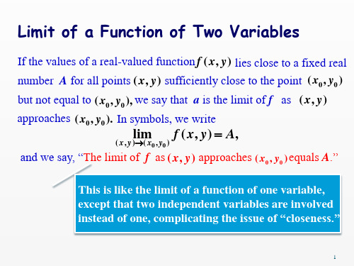
We write
lim f ( x, y) A,
( x, y)( x0 , y0 )
and assume ( x0, y0 ) is an accumulation point of the domain of f.
lim f ( x, y) A,
( x, y)( x0 , y0 )
and we say, “The limit of f as ( x, y) approaches ( x0 , y0 ) equals A.”
This is like the limit of a function of one variable, except that two independent variables are involved instead of one, complicating the issue of “closeness.”
高等数学课件详细

多元微积分的应用实例
物理学:描述物理现象,如流体力学、电磁学等 工程学:解决工程问题,如结构分析、控制系统设计等 经济学:分析经济模型,如市场均衡、最优化问题等 计算机科学:用于图像处理、机器学习等领域
无穷级数与常微分
07
方程
无穷级数的概念和性质
性质:收敛性、发散 性、绝对收敛性、条
件收敛性等
数
常微分方程的概念和分类
常微分方程:描述函数在某点或某区 间上的变化规律的方程
一阶常微分方程:只含有一个未知函 数和一个自变量的方程
二阶常微分方程:含有两个未知函数 和两个自变量的方程
高阶常微分方程:含有多个未知函数 和多个自变量的方程
线性常微分方程:未知函数和自变量 之间的关系是线性的方程
非线性常微分方程:未知函数和自变 量之间的关系是非线性的方程
常微分方程的基本解法与实例
基本解法:分离变量法、积分因子法、常数变易法等 实例:求解一阶线性常微分方程、求解二阶线性常微分方程等 应用:在物理、化学、生物等领域有广泛应用 难点:求解高阶常微分方程、求解非线性常微分方程等
微分方程的应用实例
生物:描述生物种群增长、 生态平衡等现象
化学:描述化学反应速率、 物质扩散等现象
06
多元函数微积分
多元函数的极限与连续性
多元函数的极限:定义、性质、计算方法 多元函数的连续性:定义、性质、判断方法 多元函数的可微性:定义、性质、判断方法 多元函数的可导性:定义、性质、判断方法 多元函数的可积性:定义、性质、判断方法 多元函数的积分:定义、性质、计算方法
偏导数与全微分
性质。
函数连续性的 性质:连续函 数具有局部有 界性、局部保 号性、局部保 序性等性质。
高数双语课件section1_5.pptx

kind [第一类间断点] of the function; all other discontinuous points are called discontinuity of the second kind[第二类间断点].
y
y
O
x
First kind
x O
Second Kind
11
The Classification of Discontinuous Points
Finish.
7
The Continuity of Function
2x 1, 1 x 0
Example
Prove
f
(
x
)
x
2
3,
0 x1
does not continuous at
x0 .
Proof Since f (0) 3 and
xlim0 f ( x) xlim0( x2 3) 3 f (0)
x) sin( x0)
2cos
x0
x 2
sin
x 2
then
lim
x0
y
2
lim cos
x0
x0
x 2
sin
x 2
0.
Hence sin x is continuous at x x0. Since, x0 is arbitrary point
in the interval (,), we have sin x C(,) .
(
x0
)
x x0
lim
x x0
f (x) f (x)
f ( x0)
.
f ( x0)
4
The Continuity of Function
高数双语课件section3_2.pptx

F ( x) F ( x) F ( x0 ) F ( ) f ( ) , G( x) G( x) G( x0 ) G( ) g( ) where lies between x0 and x .
x
.
SolutionIt is easy to check that the conditions of L’Hospital’s rules are satisfied for the function x sin x and x3. By L’Hospital’s rules, we have
cos x
we have
lim x lnsin
x0
x2 lim
x
lim x0
0.
ln sin 1 x
x
lim
x0
sin x
1 x2
x0 sin x
Thus,
lim (sin x)x e xlim0 xlnsin x e0 1.
x0
Finish.
13
Indeterminate Forms
means So, Finish.
f ( x)
lim
A
xx0 g( x)
f ( )
lim
x x0
g( )
A
.
f (x)
F(x)
f ( )
lim
x x0
g( x)
lim
x x0
G( x)
lim
上海财经大学英语高数课件03

f (a)(x a) f which is what we wanted to prove. . (c)(x a) For the case where x < a,we have f'(c) < f'(a), but multiplication by the negative number x - a reverses the inequality, so we get (3) and (4) as before.
Since f '(3) = 0 and f "(3) >0,f (3) = -27 is a local minimum. The point (0,0) is an inflection point since the curve changes from concave upward to concave downward there. Also (2, -16) since the curve changes from concave downward to concave upward there.
f ( x2 ) f ( x1 ) f (c)(x2 x1 )
This shows that f is increasing on [a,b]. It is similar to prove (b).
f ( x2 ) f ( x1 ) 0
or f ( x1 ) f ( x2 ).
(2) DEFINITION A point P on a curve is called a point of inflection if the curve changes from concave upward to concave downward or from concave downward to concave upward at P.
(高等数学英文课件)Some exercises of CHAPTER 2

目录 上页 下页 返回 结束
P159 40.
Analysis
f0limf0hf0...
h 0
h
f 0 02 f 0 0
f0 lim f0 h f0 lim fh
h 0
h
h 0 h
h2 f h h 2
h
h
h
目录 上页 下页 返回 结束
P159 40.
Analysis
f0limf0hf0
3. Horizontal Asymptotes
alxi m fxx,blxi m fxax
yaxb
目录 上页 下页 返回 结束
P123
60. Asymptotes
f
x
x3 x2 1 x2 1
1. Horizontal Asymptotes
limf x ...
x
2. Vertical Asymptotes
rx2000011x
1. 销量为100台的边际收益.
rx20000x2 r100 2
2. 用收益函数的导数来估计当销量从每周100台增加 到每周101台时所产生的额外的收益.
r r100
3. 计算极限并解释经济意义.
lim rxlim 2 0 0 0 0x20
x
x
目录 上页 下页 返回 结束
x
2. Vertical Asymptotes
limf x x0
x?
3. Horizontal Asymptotes
a
lim x
f
x
x
lxim
2sinx x
1 x2
0
目录 上页 下页 返回 结束
P132 6.
2.1Output, the stock market and interest rate

American Economic AssociationOutput, the Stock Market, and Interest RatesAuthor(s): Olivier J. BlanchardSource: The American Economic Review, Vol. 71, No. 1 (Mar., 1981), pp. 132-143Published by: American Economic AssociationStable URL: /stable/1805045Accessed: 28/01/2010 09:24Your use of the JSTOR archive indicates your acceptance of JSTOR's Terms and Conditions of Use, available at/page/info/about/policies/terms.jsp. JSTOR's Terms and Conditions of Use provides, in part, that unless you have obtained prior permission, you may not download an entire issue of a journal or multiple copies of articles, and you may use content in the JSTOR archive only for your personal, non-commercial use.Please contact the publisher regarding any further use of this work. Publisher contact information may be obtained at/action/showPublisher?publisherCode=aea.Each copy of any part of a JSTOR transmission must contain the same copyright notice that appears on the screen or printed page of such transmission.JSTOR is a not-for-profit service that helps scholars, researchers, and students discover, use, and build upon a wide range of content in a trusted digital archive. We use information technology and tools to increase productivity and facilitate new forms of scholarship. For more information about JSTOR, please contact support@.American Economic Association is collaborating with JSTOR to digitize, preserve and extend access to TheAmerican Economic Review.。
- 1、下载文档前请自行甄别文档内容的完整性,平台不提供额外的编辑、内容补充、找答案等附加服务。
- 2、"仅部分预览"的文档,不可在线预览部分如存在完整性等问题,可反馈申请退款(可完整预览的文档不适用该条件!)。
- 3、如文档侵犯您的权益,请联系客服反馈,我们会尽快为您处理(人工客服工作时间:9:00-18:30)。
d 3 y d d 2 f ( x) d 3 f ( x) 3 3 f ' ' ' ( x) y ' ' ' 3 ( ) D f ( x ) D x f ( x) 2 3 dx dx dx dx
up down return end
And we can define f' ' ' ' (x)=[f ' ' ' (x)] '. From now on instead of using f' ' ' ' (x) we use f(4)(x) to represent f ' ' ' ' (x). In general, we define f(n)(x)=[f(n-1)(x)] ', which is called the nth derivative of f(x). We also like to use the following notations, if y=f(x),
up
down
return
end
Corollary: If the differential of f(x) is df(x)= A(x) x,
then f(x) is differentiable and A(x)=f '(x).
Proof: From the definition,
f (t ) f ( x) A( x)t B(t , x) f ' ( x) lim lim A( x). tx t 0 tx t
up down return end
Example Use differentials to find an approximate (65)1/3 .
From definition of the differential, we can easily get
If f(x) is differentiable at x=a, and x is very closed to a, then f(x) f(a)+f '(a)(x-a). The approximation is called Linear approximation or tangent line approximation of f(x) at a. And function L(x)= f(a)+f '(a)(x-a) is called the linearization of f(x) at a.
(b) Find the equation of the tangent to the curve x3+y3 =28 at point (1,3).
up
down
return
end
Example (a) If x3+y3 =6xy, find y'. (b) Find the equation of the tangent to the folium of Descartes x3+y3 =6xy at point (3,3).
d 2 y d df ( x) d 2 f ( x) 2 2 f ' ' ( x) y ' ' 2 ( ) D f ( x ) D x f ( x) 2 dx dx dx dx
Similarly f ' ' ' (x)=[f '' (x)] '
of f(x), and
is called the third derivative
2.9 Differentials, Linear and Quadratic Approximations
Definition: Let x=x-x0, f(x) =f(x)-f(x0). If there
exists a constant A(x0) which is independent of x and x such that f(x)=A(x0) x+B(x, x0) where
f(x)cos[ xf ( x)]-2 x y cos(xy) 2 x f ' ( x) 2 2 3[ f ( x)] xcos[xf ( x)] 3 y x cos(xy)
up down return end
Example (a) If
x3+y3
=27, find
dy . dx
Corollary: (a) If f(x)=x, then dx=df(x)=x.
(b) If f(x) is differentiable, then differential
of f(x) exists and df(x)=f '(x)dx.
up
down
return
end
Example (a) Find dy, if y=x3+5x4.
up down return end
3) Derivatives of implicit function Suppose y=f(x) is an implicit function defined by sin(xy)= x2+y3. Then sin[xf(x)]=x2+ [f(x)]3. From the equation, we
up
down
return
end
2.7 Higher derivatives
Derivative f' (x) of differentiable function f(x) is also a
function. If f' (x) is differentiable, then we have [f ' (x)] '. We will denote it by f ' ' (x), i.e., f' ' (x)=[f ' (x)] '. The new function f ' ' (x) is called the second derivative of f(x). If y=f(x), we also can use other notations:
Chapter 2
Derivatives
up down return end
2.6 Implicit differentiation
1) Explicit function: The function which can be
described by expressing one variable explicitly in terms of another variable (other variables) are generally called explicit function---for example, y=xtanx, or y=[1+x2+x3]1/2 , or in general y=f(x).
B(x, x 0 ) lim 0 . Then A x is called B(x, x0) satisfies x 0 x
differential of f(x) at x0. Generally A x is denoted by df(x)|x=x = A(x0) x. Replacing x0 by x, the differential 0 is denoted by df(x) and df(x)= A(x) x.
Example The equations xy=c (c0) represents a family
of hyperbolas. And the The equations x2-y2=k (k0) represents another family of hyperbolas with asymptotes y=x. Then the two families of curves are trajectores of each other.
up
down
return
end
Example Find the linearization of the function
f(x)=(x+3)1/2 and approximations the numbers (3.98) 1/2 and (4.05)1/2.
up
down
return
end
Quadratic approximation to f(x) near x=a: Suppose f(x) is a function which the second derivative
(b) Find the value of dy when x=2 and dx=0.1.
Solution:
Geometric meaning of differential of f(x), df(x)=QS
y
y=f(x) R P d=RS
o
x
x
As x=dx is very small, y=dy ,i.e., f(t)-f(x) f '(x) t.
2) Implicit function: The functions which are defined
implicitly by a relation between variables--x and y--are generally called implicit functions--- such as x2+y2 =4, or 7sin(xy)=x2+y3 or, in general F(x,y)=0.If y=f(x) satisfies F(x, f(x))=0 on an interval I, we say f(x) is a function defined on I implicitly by F(x,y)=0, or implicit function defined by F(x,y)=0 .