SAS proc mixed 过程步介绍
SAS过程步及常用语句
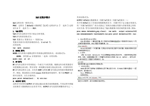
SAS过程步简介SAS过程步的一般形式为:PROC 过程名 [ DATA=输入数据集] [选项];过程语句1 [/ 选项 ];过程语句2 [/ 选项];……RUN;1.VAR语句VAR语句在过程步中用于指定分析变量。
VAR语句的语法格式为:VAR 变量名1 变量名2 … 变量名n;变量名列表可以使用省略的形式,如x1-x3 等。
应用实例:var math chinese;2.MODEL语句MODEL语句在统计建模过程中用来指定模型的形式。
语法格式为:MODEL 因变量 = 自变量列表 / 选项; 应用实例:model y=x1 x2 x3 ;3.BY语句BY语句在过程步中用来指定一个或几个分组变量,根据这些分组变量值可以把观测记录分组,然后对每一组观测分别进行指定的分析。
在使用带有BY语句的过程步之前,应先用SORT过程按BY语句指定的变量对数据集排序。
例如,假设我们已经把class1数据集按性别排序,则下面PRINT 过程可以把男、女生分别列出:proc print data=class1 ; by sex;run;4.OUTPUT语句过程步中经常用OUTPUT语句指定输出结果存放的数据集。
不同过程中把输出结果存入数据集的方法各有不同,OUTPUT语句是使用频繁的语句之一。
其语法格式为:OUTPUT OUT=输出数据集名关键字=变量名关键字=变量名…;其中用OUT=给出了存放结果数据集的名字,关键字用于定义输出变量名,用“关键字=变量名”的方式指定了系统自动输出变量与存储变量之间的对应关系。
等号后面的变量名指定了输出数据集中的存储变量名称。
例如:proc means data=data_prg.class1; var math; output out=result02 n=n mean=meanmath var=varmath;run;proc print data=result02; run;在DATA步中也可以用FORMAT语句规定变量的输出格式,用LABEL 语句规定变量的标签,用LENGTH语句规定变量的存储长度,用ATTRIB语句同时规定变量的各属性。
用SAS的mixed过程拟合林分的线性差分生长模型
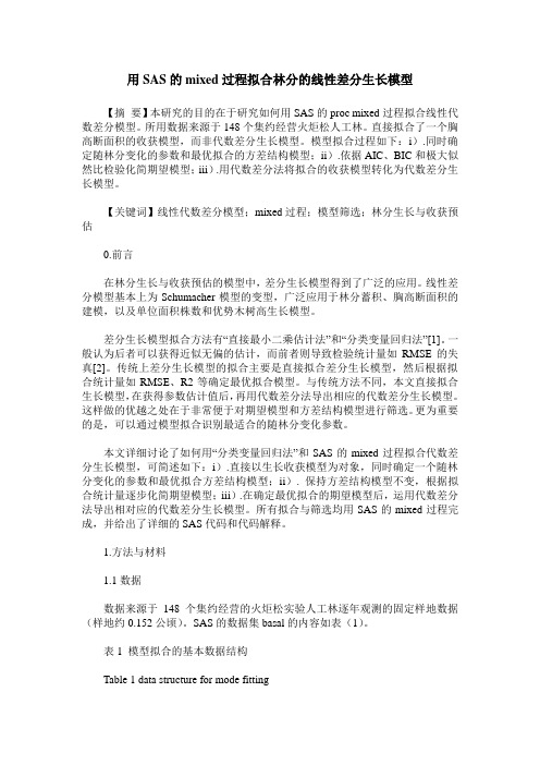
用SAS的mixed过程拟合林分的线性差分生长模型【摘要】本研究的目的在于研究如何用SAS的proc mixed过程拟合线性代数差分模型。
所用数据来源于148个集约经营火炬松人工林。
直接拟合了一个胸高断面积的收获模型,而非代数差分生长模型。
模型拟合过程如下:i).同时确定随林分变化的参数和最优拟合的方差结构模型;ii).依据AIC、BIC和极大似然比检验化简期望模型;iii).用代数差分法将拟合的收获模型转化为代数差分生长模型。
【关键词】线性代数差分模型;mixed过程;模型筛选;林分生长与收获预估0.前言在林分生长与收获预估的模型中,差分生长模型得到了广泛的应用。
线性差分模型基本上为Schumacher模型的变型,广泛应用于林分蓄积、胸高断面积的建模,以及单位面积株数和优势木树高生长模型。
差分生长模型拟合方法有“直接最小二乘估计法”和“分类变量回归法”[1]。
一般认为后者可以获得近似无偏的估计,而前者则导致检验统计量如RMSE的失真[2]。
传统上差分生长模型的拟合主要是直接拟合差分生长模型,然后根据拟合统计量如RMSE、R2等确定最优拟合模型。
与传统方法不同,本文直接拟合生长模型,在获得参数估计值后,再用代数差分法导出相应的代数差分生长模型。
这样做的优越之处在于非常便于对期望模型和方差结构模型进行筛选。
更为重要的是,可以通过模型拟合识别最适合的随林分变化参数。
本文详细讨论了如何用“分类变量回归法”和SAS的mixed过程拟合代数差分生长模型,可简述如下:i).直接以生长收获模型为对象,同时确定一个随林分变化的参数和最优拟合方差结构模型;ii). 保持方差结构模型不变,根据拟合统计量逐步化简期望模型;iii).在确定最优拟合的期望模型后,运用代数差分法导出相对应的代数差分生长模型。
所有拟合与筛选均用SAS的mixed过程完成,并给出了详细的SAS代码和代码解释。
1.方法与材料1.1数据数据来源于148个集约经营的火炬松实验人工林逐年观测的固定样地数据(样地约0.152公顷)。
20个SAS过程步
20个SAS过程步
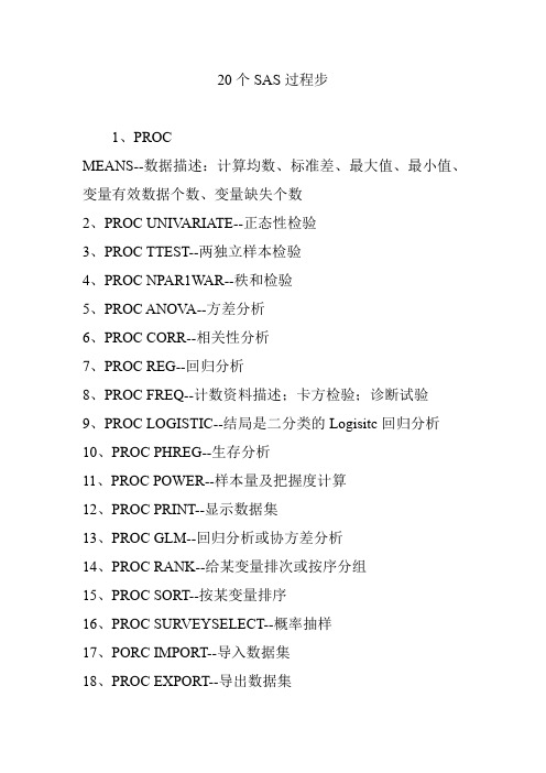
1、PROC
MEANS--数据描述:计算均数、标准差、最大值、最小值、变量有效数据个数、变量缺失个数
2、PROC UNIV ARIATE--正态性检验
3、PROC TTEST--两独立样本检验
4、PROC NPAR1WAR--秩和检验
5、PROC ANOV A--方差分析
6、PROC CORR--相关性分析
7、PROC REG--回归分析
8、PROC FREQ--计数资料描述;卡方检验;诊断试验
9、PROC LOGISTIC--结局是二分类的Logisitc回归分析
10、PROC PHREG--生存分析
11、PROC POWER--样本量及把握度计算
12、PROC PRINT--显示数据集
13、PROC GLM--回归分析或协方差分析
14、PROC RANK--给某变量排次或按序分组
15、PROC SORT--按某变量排序
16、PROC SURVEYSELECT--概率抽样
17、PORC IMPORT--导入数据集
18、PROC EXPORT--导出数据集
19、PROC CONTENTS--产生一个数据集的头文件,包含了多种该数据集的信息
20、PROC TABULATE--输出报表。
SAS过程简介
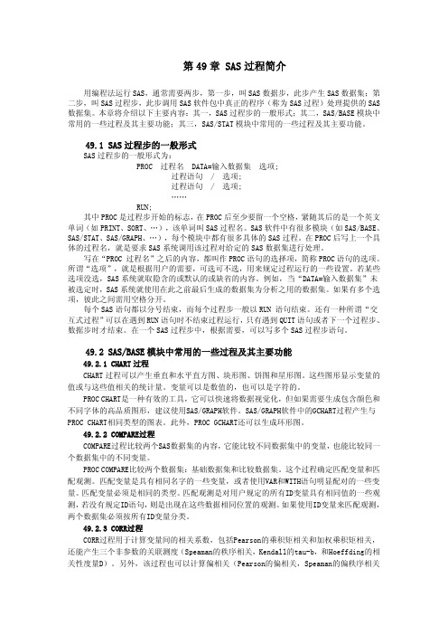
第49章 SAS过程简介用编程法运行SAS,通常需要两步,第一步,叫SAS数据步,此步产生SAS数据集;第二步,叫SAS过程步,此步调用SAS软件包中真正的程序(称为SAS过程)处理提供的SAS 数据集。
本章将介绍以下主要内容:其一,SAS过程步的一般形式;其二,SAS/BASE模块中常用的一些过程及其主要功能;其三,SAS/STAT模块中常用的一些过程及其主要功能。
49.1 SAS过程步的一般形式SAS过程步的一般形式为:PROC 过程名 DATA=输入数据集 选项;过程语句 / 选项;过程语句 / 选项;……RUN;其中PROC是过程步开始的标志,在PROC后至少要留一个空格,紧随其后的是一个英文单词(如PRINT、SORT、…),该单词叫SAS过程名。
SAS软件中有很多模块(如SAS/BASE、SAS/STAT、SAS/GRAPH、…),每个模块中都有很多具体的SAS过程。
在PROC后写上一个具体的过程名,就是要求SAS系统调用该过程对给定的SAS数据集进行处理。
写在“PROC 过程名”之后的内容,都叫作PROC语句的选择项,简称PROC语句的选项。
所谓“选项”,就是根据用户的需要,可选可不选,用来规定过程运行的一些设置。
若某些选项没选,SAS系统就取隐含的或默认的或缺省的内容。
例如,当“DATA=输入数据集”未被选定时,SAS系统就使用在此之前最后生成的数据集为分析之用的数据集。
如果有多个选项,彼此之间需用空格分开。
每个SAS语句都以分号结束,而每个过程步一般以RUN 语句结束。
还有一种所谓“交互式过程”可以在遇到RUN语句时不结束过程运行,只有遇到QUIT语句或者下一个过程步、数据步时才结束。
在一个SAS过程步中,根据需要,可以写多个SAS过程步语句。
49.2 SAS/BASE模块中常用的一些过程及其主要功能49.2.1 CHART过程CHART过程可以产生垂直和水平直方图、块形图、饼图和星形图。
proc mixed 误差项 sas 混合模型 公式

proc mixed 误差项sas 混合模型公式全文共四篇示例,供读者参考第一篇示例:PROC MIXED是SAS中用于混合模型分析的过程,混合模型是一种能够处理多层次结构或者重复测量数据的统计模型。
在混合模型中,我们可以同时考虑固定效应和随机效应,进而对不同层次的变量进行分析。
在混合模型中,误差项扮演着非常重要的角色,它是模型中必不可少的一个组成部分。
本文将介绍关于PROC MIXED中误差项的相关知识,并给出相应的混合模型公式。
误差项在混合模型中是指未被模型中的自变量所解释的部分,也就是模型中未被考虑的随机误差。
在混合模型中,我们通常假设误差项服从正态分布,并且具有均值为0、方差为σ^2的特性。
误差项的存在使得我们能够量化模型中的不确定性,评估模型的拟合程度,并且进行相关的统计推断。
在PROC MIXED中,我们可以通过指定各种固定效应和随机效应来构建混合模型。
常见的混合模型可以被表达为如下的公式:Y = Xβ + Zγ + εY表示观测到的因变量向量,X是固定效应矩阵,β是固定效应参数向量,Z是随机效应矩阵,γ是随机效应参数向量,ε是误差项向量。
在该公式中,固定效应表示各个因素对因变量的整体影响,而随机效应则表示了在样本中的个体差异。
误差项则是模型中未被解释的残差部分。
在具体的数据分析过程中,我们需要根据研究的实际情况来构建混合模型。
在进行实验设计时,我们需要考虑实验中的重复测量数据或者样本数据的层次结构。
在这种情况下,混合模型能够更好地分析不同层次之间的关系,并且考虑到各个层次的变异性。
通过PROC MIXED进行混合模型分析时,我们可以通过设定不同的协方差结构来进一步扩展模型的适用范围。
可以选择不同的协方差结构来描述不同层次的数据之间的相关性。
PROC MIXED还提供了丰富的选项来进行模型拟合和参数估计,包括最大似然估计、重复测量设计、协变量调整等功能。
第二篇示例:混合模型是一种在统计分析中常用的模型,特别是当研究对象存在多个层次或重复测量时。
SAS分析常用的过程过程步大全
SAS分析常用的过程过程步大全为区分过程名称的拼写,故意部分小写,以便识别和记忆。
基本SAS程序代码结构:---------PROC MODE data=Arndata.moddat; /* 命令的解释*/var y x1-x6; /* 命令的解释 */model y = x1-x6;run;------------------------------------------正态性检验PROC UNIvariate---------PROCUNIvariate data=Arndata.unidat;var x1;run;------------------------------------------相关分析和回归分析PROC REG 回归---------PROC REG data=Arndata.regdat;var y x1-x6;model y = x1-x6 / selection=stepwise;/* 加入逐步回归选项 */print cli; /* 加入输出预测结果部分,还可以输出acov,all,cli,clm,collin,collinoint,cookd,corrb,covb,dw(时序检验统计量),i,influence,p,partial,pcorr1,pcorr2,r,scorr1,scorr2,seqb,spec,ss1,ss2,stb,tol, vif(异方差检验统计量),xpx*/plot y*x2 / conf95; /* 做散点图 */run;---------------------------------------------------DATA Arndata.regdat;x2x2 = x2*x2;x1x2 = x1*x2;PROC REG data=Arndata.regdat;var y x1 x2 x2x2 x1x2 ; /* 多项式回归,非线性回归 */model y = x1 x2 x2x2 x1x2 / selection=stepwise; /* 加入逐步回归选项*/print cli;plot y*x2 / conf95; /* 做散点图 */run;------------------------------------------PROC RSreg 二次响应面回归PROC ORTHOreg 病态数据回归PROC NLIN 非线性回归PROC TRANSreg 变换回归PROC CALIS 线性结构方程和路径分析PROC GLM 一般线性模型PROC GENmod 广义线性模型方差分析PROC ANOVA 单因素均衡数据和非均衡数据---------PROC ANOVA data=Arndata.anovadat; /* 命令的解释 */class typ; /* 命令的解释 */model y = typ; /* 可以看出此处是单因素方差分析(分类型自变量对数值型自变量的影响) */run;------------------------------------------PROC GLM 多因素非均衡数据:---------PROC GLM data=Arndata.glmdat; /* 命令的解释*/class typea typeb; /* 命令的解释 */model y = typea typeb; /* 可以看出此处是不考虑交互作用的多因素方差分析(分类型自变量对数值型自变量的影响) */run;---------------------------------------------------PROC GLM data=Arndata.glmdat; /* 命令的解释*/class typea typeb; /* 命令的解释 */model y = typea typeb typea*typeb; /* 可以看出此处是考虑交互作用的多因素方差分析(分类型自变量对数值型自变量的影响) */run;------------------------------------------主成分分析PROC PRINcomp---------PROCPRINcomp data=Arndata.pmdat n=4 out=w1 outstat=w2 ;var x1-x6;PROC print data=w1;PROC plot data=w1 vpct=80; /* 一句话,其实print就是plot输出图形的文字形式而已 */plot prin1*prin2 $ districts='*'/haxis=-3.5 to 3 by 0.5 HREF=-2,0,2vaxis=-3 to 4.5 by 1.5 HREF=-2,0,2; /* 主成分的散点图,也就是载荷图 */run;------------------------------------------因子分析PROC FACTOR---------PROC FACTOR data=Arndata.factordat simple corr ;var y x1-x6;title'18个财务指标的分析';title2'主成分解';run;PROC FACTOR data=Arndata.factordatn=4 ; /* 选择4个公共因子 */ var y x1-x6;run;PROC FACTOR data=Arndata.factordat n=4rotate=VARImaxREorder; /* 因子旋转:方差最大因子法 */var y x1-x6;run;------------------------------------------PROC SCORE---------PROC FACTOR data=Arndata.factordat n=4rotate=VARImax REorder score out=score_Out; /* 输出因子得分矩阵 */run;PROC print data=score_Out;var districts factor1 factor2 factor3 factor4;run;PROC plot data=score_Out;plot factor1*factor2 $ districts='*' / href=0 Vref=0; /* 因子的散点图,也就是载荷图 */run;------------------------------------------典型相关分析PROC CANcorr基本SAS程序代码结构:---------DATAjt(TYPE=CORR); /*TYPE=CORR 表明数据类型为相关矩阵,而不是原始数据, type还可以是cov,ucov,factor,sscp,ucorr等*/input names$ 1-2(x1 x2 y1-y3)(6.); /* name $ 表示读取左侧的变量名,1-2表示变量名的字符落在第1,2列上 */cards;x1 1 0.8 ……x2 ……y1 ……y2 ……y3 ……;PROC CANcorrdata=Arndata.cancorrdatedf=70 redundancy; /* 误差自由度的参考值,默认值是n=1000;redundancy表示输出冗余度分析的结果 */var x1 x2;with y1 y2 y3;run;------------------------------------------对应分析 /* 交叉表分析的拓展,寻找行和列的关系,一般行指代各种cases,而列代表各种visions */PROC CORResp---------PROC CORRespdata=Arndata.correspdat out=result;var x1-x6;id Type;run;options ps=40;proc plot data=result;plot dim2*dim1="*" $ Type / boxhaxis=-0.2 to 0.3 by 0.1Vaxis=-0.1 to 0.3 by 0.1Href=0 Vref=0;run;------------------------------------------聚类分析PROC CLUSTER---------PROC CLUSTER data=Arndata.clusdatmethod=ave outtree=clusdat_Out;var x1-x6;id datid;run;proc tree horizontal; /* 做聚类树 */run;------------------------------------------PROC FASTclus---------PROC FASTclus data=Arndata.clusdatmaxclusters=3 list out=clusdat_Out;var x1-x6;id datid;run;------------------------------------------PROC ACEclusPROC VARCLUS---------PROC VARclus data=Arndata.clusdat;/* 系统默认使用主成分法聚类 */var x1-x6;run;---------PROC VARclus hierarchy data=Arndata.clusdat; /* 保证分析过程中不同水平的谱系结构 */var x1-x6;run;---------PROC VARclus centroid data=Arndata.clusdatouttree=clusdat_out; /* 使用重心法聚类 */ var x1-x6;run;------------------------------------------PROC TREE---------PROC TREE data=Arndata.clusdat horizontal; /* 使用TREE过程绘制聚类谱系图*/var x1-x6;run;------------------------------------------判别分析PROC DISCRIM---------PROC DISCRIM data=Arndata.discrimdatlist out=discrimdat_Out distance pool=yes;class Typ; /* 指定分类变量 */var x1-x6; /* 用于建立判别识别函数的变量 */id iddiscrim; /* 标注样本的变量 */run;---------第二种方法,将需要判别的新样本放在testdata里:---------PROC DISCRIM data=Arndata.discrimdat1testdata=Arndata.discrimdat2testlist testout=discrimdat_Out; /* 将原来的几个选项加注test标示 */class Typ; /* 指定分类变量 */var x1-x6; /* 用于建立判别识别函数的变量 */id iddiscrim; /* 标注样本的变量 */run;------------------------------------------PROC STEPdisc:逐步判别分析过程---------PROC STEPdisc method=stepwise data=Arndata.discrimdatSLentry=0.10 SLstay=0.10; /* 设定引入和剔除的显著性水平 */class Typ; /* 指定分类变量 */var x1-x6; /* 用于建立判别识别函数的变量 */run;------------------------------------------PROC CANdisc: Fisher判别分析过程---------PROC CANdiscdata=Arndata.discrimdatout=discrimdat_Outdistance simple;class Typ; /* 指定分类变量 */var x1-x6; /* 用于建立判别识别函数的变量 */run;proc print data=discrimdat_Out;run;-----------------------------------------------------------------------------------------------------------------------------------------------------------友情协助:特征库豆瓣统计学小组 /group/stats。
第21章 SAS过程步操作基础

means过程可计算的统计量(一)
关键字
N NMISS MEAN STD STDERR VAR MEDIAN CV
所代表的含义
有效数据记录数 缺失数据记录数 均数 标准差 标准误 方差 中位数 变异系数
关键字
MAX MIN RANGE SUM SUMWGT CSS USS CLM
所代表的含义
最大值 最小值 全距 总计 加权总计 校正的离均差平方和 未校正的离均差平方和 可信限(上、下界值)
contents过程
contents过程用于显示指定的SAS数据集的有关信息 或者相应逻辑库中所包含成员的列表信息。 对于指定的SAS数据集,contents过程将列出数据集 的各种属性信息,以及所包含的全部变量及其属性。 有关变量信息的列表将按照字母顺序排列,变量属性 信息包括变量类型、长度、标签以及格式等。 contents过程的一般形式如下: proc contents data=SAS-data-set options; run;
means过程示例
data test;
do i=1 to 3; do j=1 to 2; do k=1 to 30; x=abs(ranuni(0))*10+8;
y=x**1.5;
output; end; end; end;
run;
proc means data=test mean median std var cv t probt; class i j; var x y; output out=outdata mean(x y)=mx my std(x y)=sx xy; run;
print过程支持的其它语句
proc mixed 置信区间
proc mixed 置信区间一、介绍proc mixed 是SAS 软件中的一个过程,用于拟合混合线性模型。
在统计分析中,经常需要对模型参数进行置信区间估计,以评估变量之间的关系是否显著。
本文将介绍如何使用proc mixed 进行置信区间估计,并解释置信区间的含义和解读方法。
二、置信区间的概念置信区间是对参数估计的不确定性进行度量的一种方法。
在回归分析中,我们通常对模型中的系数进行估计,例如斜率和截距。
通过计算置信区间,我们可以得到一个区间,该区间内的真实参数值有一定的概率落在其中。
置信区间的计算基于样本数据和统计理论,其中最常用的方法是基于正态分布的置信区间。
在proc mixed 中,默认使用的是95%的置信区间,即我们希望真实参数值在计算出的区间内的概率为95%。
三、使用 proc mixed 进行置信区间估计使用 proc mixed 进行置信区间估计的步骤如下:1. 导入数据:首先需要将数据导入SAS 软件中,可以使用data step 或者 proc import 进行数据导入。
2. 定义模型:使用proc mixed 过程,通过指定固定效应和随机效应来定义混合线性模型。
例如,可以使用类别变量作为固定效应,使用随机效应来建模不同个体之间的差异。
3. 估计参数:使用proc mixed 进行模型的拟合和参数估计。
拟合过程将生成各个模型参数的估计值。
4. 计算置信区间:使用estimate 语句在proc mixed 中计算置信区间。
可以通过指定 alpha 参数来控制置信水平,默认为0.05。
5. 解读结果:根据计算得到的置信区间,可以判断模型中的变量之间是否存在显著差异。
如果置信区间包含零,则说明差异不显著;如果置信区间不包含零,则说明差异显著。
四、置信区间的解读置信区间提供了一种度量参数估计的不确定性的方法。
通常情况下,我们希望置信区间越窄越好,因为窄的置信区间意味着对参数估计的确定性更高。
- 1、下载文档前请自行甄别文档内容的完整性,平台不提供额外的编辑、内容补充、找答案等附加服务。
- 2、"仅部分预览"的文档,不可在线预览部分如存在完整性等问题,可反馈申请退款(可完整预览的文档不适用该条件!)。
- 3、如文档侵犯您的权益,请联系客服反馈,我们会尽快为您处理(人工客服工作时间:9:00-18:30)。
Introduction to PROC MIXEDTable of Contents1.Short description of methods of estimation used in PROC MIXED2.Description of the syntax of PROC MIXED3.References4. Examples and comparisons of results from MIXED and GLM- balanced data: fixed effect model and mixed effect model,- unbalanced data, mixed effect model1. Short description of methods of estimation used in PROC MIXED.The SAS procedures GLM and MIXED can be used to fit linear models. Proc GLM was designed to fit fixed effect models and later amended to fit some random effect models by including RANDOM statement with TEST option. The REPEATED statement in PROC GLM allows to estimate and test repeated measures models with an arbitrary correlation structure for repeated observations. The PROC MIXED was specifically designed to fit mixed effect models. It can model random and mixed effect data, repeated measures, spacial data, data with heterogeneous variances and autocorrelated observations.The MIXED procedure is more general than GLM in the sense that it gives a user more flexibility in specifying the correlation structures, particularly useful in repeated measures and random effect models. It has to be emphasized, however, that the PROC MIXED is not an extended, more general version of GLM. They are based on different statistical principles; GLM and MIXED use different estimation methods. GLM uses the ordinary least squares (OLS) estimation, that is, parameter estimates are such values of the parameters of the model that minimize the squared difference between observed and predicted values of the dependent variable. That approach leads to the familiar analysis of variance table in which the variability in the dependent variable (the total sum of squares) is divided into variabilities due to different sources (sum of squares for effects in the model). PROC MIXED does not produce an analysis of variance table, because it uses estimation methods based on different principles. PROC MIXED has three options for the method of estimation. They are: ML (Maximum Likelihood), REML (Restricted or Residual maximum likelihood, which is the default method) and MIVQUE0 (Minimum Variance Quadratic Unbiased Estimation). ML and REML are based on a maximum likelihood estimation approach. They require the assumption that the distribution of the dependent variable (error term and the random effects) is normal. ML is just the regular maximum likelihood method,that is, the parameter estimates that it produces are such values of the model parameters that maximize the likelihood function. REML method is a variant of maximum likelihood estimation; REML estimators are obtained not from maximizing the whole likelihood function, but only that part that is invariant to the fixed effects part of the linear model. In other words, if y = X b + Zu + e, where X b is thefixed effects part, Zu is the random effects part and e is the error term, then the REML estimates are obtained by maximizing the likelihood function of K'y, where K is a full rank matrix with columns orthogonal to the columns of the X matrix, that is, K'X= 0. It leads to REML estimator of the variance-covariance matrix of y, say V. It does not depend on the choice of matrix K. Then the generalized least squares equations, known also from the weighted least squares approach and the GLM procedure,X'(inverse of V)X b=X'(inverse of V)y,where V is replaced with its estimator, are solved to obtain the estimates of fixed effects parameters b.It is assumed that the random effects u and the error vector e are normally distributed, uncorrelated and have expectations 0. Under the assumption that u and e are not correlated, V, the variance-covariance matrix of y, is equal to ZGZ’ + R, where G and R are the variance matrices of u and e, respectively.Estimators of V, the variance-covariance matrix of y, can also be obtained in PROC MIXED by the MIVQUE0 method. For a short description of the method see reference (3), p.506. This method has two advantages over ML and REML; it does not require normality assumption (for computing the estimators) as do ML and REML and does not involve iterations. However simulation studies by Swallow and Monahan (1984) present evidence favoring ML and REML over MIVQUE0. PROC MIXED uses MIVQUE0 as starting values for the ML and RELM procedures.For balanced data the REML method of PROC MIXED provides estimators and hypotheses test results that are identical to ANOVA (OLS method of GLM), provided that the ANOVA estimators of variance components are not negative. The estimators, as in GLM, are unbiased and have minimum variance properties. The ML estimators are biased in that case. In general case of unbalanced data neither the ML nor the REML estimators are unbiased and they do not have to be equal to those obtained from PROC GLM. There are many models involving forms of variance-covariance structure of observations that can not be analyzed using PROC GLM with TEST or PROC GLM with the REPEATED options. PROC MIXED can handle such cases. It also has to be mentioned that PROC GLM was design for analysis of fixed effects models and all computations are done under the assumption that there is only one variance component in the model, the error term. The RANDOM statement with the TEST option can be used to get the right tests in the case random effects are present in the model, but still some printed results, variances and standard errors, will be incorrect.2. Description of the syntax of PROC MIXEDThe PROC MIXED syntax is similar to the syntax of PROC GLM. There are, however, a few important differences. The random effects and repeated statements are used differently, random effects are not listed in the model statement, GLM has MEANS and LSMEANS statements, whereas MIXED has only the LSMEANS statement, GLM offers Type I, II, III and IV tests for fixed effects, while MIXED offers TYPE I and TYPE III. The following is a general form of PROC MIXED statement: PROC MIXED options;CLASS variable-list;MODEL dependent=fixed effects/ options;RANDOM random effects / options;REPEATED repeated effects / options;CONTRAST 'label' fixed-effect values | random-effect values/ options;ESTIMATE 'label' fixed-effect values | random-effect values/ options;LSMEANS fixed-effects / options;MAKE 'table' OUT= SAS-data-set < options >;RUN;The CONTRAST, ESTIMATE, LSMEANS, MAKE and RANDOM statements can appear multiple times, all other statements can appear only once.The PROC MIXED and MODEL statements are required. The MODEL statement must appear after the CLASS statement if CLASS statement is used. The CONTRAST, ESTIMATE, LSMEANS, RANDOM and REPEATED statement must follow the MODEL statement. CONTRAST and ESTIMATE statements must follow RANDOM statement if the RANDOM is used.A detailed description of all functions and options of each PROC MIXED statement is given inSAS/STAT Software Changes and Enhancements through Release 6.11 and SAS/STAT Software Changes and Enhancements for Release 6.12, SAS Institute Inc. (1996). The following is a short summary of selected, most often used, MIXED procedure statements.PROC MIXED <options>;Selected options:DATA= SAS data setNames SAS data set to be used by PROC MIXED. The default is the most recently created data set. METHOD=REMLMETHOD=MLMETHOD=MIVQUE0Specifies the estimation method. See Section 1 for a brief description of the methods and references. REML is the default method.COVTESTPrints asymptotic standard errors and Wald Z-test for variance-covariance structure parameter estimates. For example, if a random effect A is included in the model, then the estimator of the variance of A will be printed together with the Wald test of the hypothesis that the variance of A is 0.The COVTEST option is specified after Proc mixed and before semicolon;. For example,Proc mixed data=mydata method=reml covtest;CLASS variables;Lists classification variables (categorical independent variables in the model). For example:proc mixed data=mydata covtest;Class group gender agecat;MODEL dependent = fixed effects </options>;The model statement names a single dependent variable and the fixed effects, that is independent variables that are not random. An intercept is included in the model by default. The NOINT option can be used to remove the intercept.NOTE: Even though PROC MIXED allows only for one dependent variable in the model statement, it is possible to use it to model, for example, multivariate repeated measures. In such case, the data set has to be properly prepared and should contain a variable indicating the measurement type. The correlation between observations on the same unit has to be modeled properly with the REPEATED statement. For example, suppose your observed data consist of heights and weights of children measured over several successive years. Your input data set should then contain variables similar to the following:Y, all of the heights and weights, with a separate observation (line in the data file) for eachVAR, indicating whether the measurement is a height or a weightYEAR, indicating the year of measurementCHILD, indicating the child on which the measurement was taken.Selected Options of the model statement:CHISQ, request χ2 – tests (Wald tests) be performed for all fixed effects in addition to the F-tests. DDFM=RESIDUALDDFM=CONTAINDDFM=BETWITHNDDFM=SATTERTH,The DDFM= options specifies the method for computing the denominator degrees of freedom for the tests of fixed effects. DDFM=SATTERTH will result in the Satterthwaite approximation for the denominator degrees of freedom. For balanced designs with random effects it will produce the same test results as RANDOM …/ TEST option in PROC GLM (if the default METHOD=REML is used in proc mixed).P, requests that the predicted values be printed.RANDOM random effects </options>;The RANDOM statement defines the random effects in the model. It can be used to specify traditional variance components (independent random effects with different variances) or to list correlated random effects and specify a correlation structure for them with the TYPE=covariance-structure option. A variety of structures are available (see references 5 and 6), most often used are either TYPE=VC, a variance components correlation structure or TYPE=UN, an unstructured, that is, arbitrary covariance matrix. TYPE=VC is the default structure. In the following example, the effect of subject is random.Proc mixed data=one method=reml covtest;Class gender treat subject;Model y=gender treat gender*treat /ddfm=satterth;Random subject(gender);Run;In the next example there are two random effects specified (besides the error term) and it is assumed that they are correlated.Intercept and the slope coefficient in the regression equation have fixed and random parts which are assumed to be correlated. The model is:yij = a0 +aj + b0*time + bj*time + eij, where yij is observation i for person j.The random effects, aj, bj and eij, are asumed to have normal distributions with mean zero and different variances and it is also assumed that aj and bj are correlated.Proc mixed data=one method=reml covtest;Class person;Model y=time /solution;Random intercept time /type=un subject=person;Run;REPEATED repeated effects / options;The repeated statement is used in PROC MIXED to specify the covariance structure of the error term. The repeated effect has to be categorical and has to appear in the class statement and the data has to be sorted accordingly. For example, suppose that for each subject a measurement was taken at five equally spaced time points. The time is the repeated effect and the data has to be sorted by subject and time within each subject. If time is also used as a continuous independent variable in the model then a new variable, say t, identical to time has to be defined and t should be used in the class and repeated statements. For example:Data one;Set one;T=time;Run;Proc sort data=one;By group id t;Run;Proc mixed data=one covtest;Class t group id;Model y=group time group*time;Repeated t /type=ar(1) subject=id;Run;The option TYPE in the REPEATED statement specifies the type of the error correlation structure. The one specified in the above example is the first-order autoregressive correlation. The subject option is needed to identify observations that are correlated. Observations within the same subject are correlated with the type of correlation specified in TYPE, observations from different subjects are independent.The TYPE option allows for many types of correlation structures. Most commonly used are autocorrelation, compound symmetry, Huynh-Feldt, Toeplitz, variance components, unstructured and spatial. For the complete list and examples, see references (7) and (8).CONTRAST ‘label’ fixed-effect values | random-effect values / options;ESTIMATE ‘label’ fixed-effect values | random-effect values / options;The CONTRAST statement is used when there is need for custom hypothesis tests, the ESTIMATE statement, when there is need for custom estimates. Although they were extended in PROC MIXED to include random effects, their use is very similar to the CONTRAST and ESTIMATE statement in PROC GLM.LABEL is required for every contrast or estimate statement. It identifies the contrast or estimated parameter on the output. It can not be longer than 20 characters.FIXED-EFFECT is the name of an effect appearing in the MODEL statement.RANDOM-EFFECT is the name of an effect appearing in the RANDOM statement.VALUES are the coefficients of the contrast to be tested or the parameter to be estimated.For example, suppose that we want to test if there is a significant effect of treat in group 2, where treat has three levels and group four levels. We also want to estimate the mean for treat 1 in group 2, the mean for treat 2 in group 2 and the difference between these two means. We will need the following CONTRAST and ESTIMATE statements to obtain these results.Proc mixed data=one method=reml covtest;Class group treat subject;Model y=group treat group*treat /ddfm=satterth;Random subject(group);Contrast ‘treat in group 2’Treat 1 –1 0 group*treat 0 0 0 1 –1 0 0 0 0 0 0 0,Treat 0 1 –1 group*treat 0 0 0 0 1 –1 0 0 0 0 0 0;Estimate ‘treat1 group2 mean’ intercept 1 group 0 1 0 0 treat 1 0 0group*treat 0 0 0 1 0 0 0 0 0 0 0 0;Estimate ‘treat2 group2 mean’ intercept 1 group 0 1 0 0 treat 0 1 0Group*treat 0 0 0 0 1 0 0 0 0 0 0 0;Estimate ‘mean diff t1g2-t2g2’ Treat 1 –1 0 group*treat 0 0 0 1 –1 0 0 0 0 0 0 0;Run;LSMEANS fixed-effects / options;LSMEANS computes the least squares means of fixed effects. The ADJUST option requests a multiplecomparison adjustment to the p-values for pair-wise comparisons of means. The following adjustments are available: BON (Bonferroni), DUNNET, SCHEFFE, SIDAK, SIMULATE, SMM|GT2 and TUKEY. The ADJUST option results in all possible pair-wise comparisons. If comparisons with a control level are only needed then in addition to ADJUST option, PDIFF=control should be used. The SLICE option allows to test the significance of one effect at each level of another effect.For example, suppose that we want to compute the least squares means for group*treat and do pair-wise comparisons with the control being group 1 and treat 1. We also want to test for the significance of the treat effect within each group level using the SLICE option..Proc mixed data=one method=reml covtest;Class group treat subject;Model y=group treat group*treat /ddfm=satterth;Random subject(group);lsmeans group*treat /adjust=bon pdiff=control('1' '1') slice=group;Run;MAKE 'table' OUT= SAS-data-set < options >;The MAKE statement converts any table produced by PROC MIXED into a sas data set. NOPRINT option can be used to prevent printing the requested table. Only requested or default output can be converted into a sas data set. Hence, in particular, the P option has to be used in the model statement to produce a data set with predicted values, and the LSMEANS statement has to be included to output least squares means. For example,Proc mixed data=one method=reml covtest;Class group treat subject;Model y=group treat group*treat /ddfm=satterth p;Random subject(group);lsmeans group*treat /adjust=bon pdiff=control('1' '1') slice=group;make ‘LSMeans’ out=gtmeans;make ‘predicted’ out=pred noprint;Run;Proc print data=gtmeans;Proc print data=pred;Run;ReferencesStatistics Books:1. Searle, Shayle R. (1987). Linear Models For Unbalanced Data, John Wiley & Sons.2. Searle, Shayle R. (1971). Linear Models, John Wiley & Sons.3. Searle, S.R., Casella, G., and McCulloch, C.E. (1992), Variance Components. John Wiley&Sons.4. Verbeke, G., Molenberghs, G. (Editors) (1997), Linear Mixed Models in Practice. A SAS-Oriented Approach. Springer-VerlagSAS Institute Books:5. Littell, Ramon C., Milliken, George A., Stroup, Walter W., Wolfinger, Russell D. (1996). SAS System For Mixed Models, SAS Institute Inc.6. SAS Institute Course Notes (1996). Advanced General Linear Models with an Emphasis on Mixed Models, SAS Institute Inc.7. SAS/STAT Software Changes and Enhancements through Release 6.11, SAS Institute Inc. 1996.8. SAS/STAT Software Changes and Enhancements for Release 6.12, SAS Institute Inc. 1996.3. Examples and comparisons of the results from PROC MIXED and PROC GLM. Example1. Fixed effect model, balanced data.In this example, 36 subjects are randomly assigned to 12 group – treatment combinations, 3 to each combination. There are three treatments and four groups. In the following program, factor treat with 3 levels is the effect of the treatment and factor group with 4 levels is the effect of the group.As you can see below, the results from both procedures are identical.Program:options ls=76;data one;input y group treat subject;cards;22 1 1 123 1 1 225 1 1 317 1 2 418 1 2 523 1 2 612 1 3 716 1 3 814 1 3 98 2 1 109 2 1 1110 2 1 1216 2 2 1317 2 2 1420 2 2 1529 2 3 1630 2 3 1736 2 3 183 3 1 197 3 1 205 3 1 211 32 222 3 2 231 32 244 3 3 257 3 3 268 3 3 2711 4 1 2815 4 1 298 4 1 3034 4 2 3137 4 2 3233 4 2 3327 4 3 3428 4 3 3524 4 3 36;run;Proc mixed data=one method=reml;Class group treat;Model y=group treat group*treat;lsmeans group*treat /adjust=bon pdiff=control('1' '1') slice=group;Contrast 'treat in group 2'Treat 1 -1 0 group*treat 0 0 0 1 -1 0 0 0 0 0 0 0,Treat 0 1 -1 group*treat 0 0 0 0 1 -1 0 0 0 0 0 0;Estimate 'treat1 group2 mean' intercept 1 group 0 1 0 0 treat 1 0 0group*treat 0 0 0 1 0 0 0 0 0 0 0 0;Estimate 'treat2 group2 mean' intercept 1 group 0 1 0 0 treat 0 1 0Group*treat 0 0 0 0 1 0 0 0 0 0 0 0;Estimate 'mean diff t1g2-t2g2' Treat 1 -1 0 group*treat 0 0 0 1 -1 0 0 0 0 0 0 0; Run;proc GLM data=one;class group treat;Model y=group treat group*treat;lsmeans group*treat /adjust=bon pdiff=control('1' '1') slice=group;Contrast 'treat in group 2'Treat 1 -1 0 group*treat 0 0 0 1 -1 0 0 0 0 0 0 0,Treat 0 1 -1 group*treat 0 0 0 0 1 -1 0 0 0 0 0 0;Estimate 'treat1 group2 mean' intercept 1 group 0 1 0 0 treat 1 0 0group*treat 0 0 0 1 0 0 0 0 0 0 0 0;Estimate 'treat2 group2 mean' intercept 1 group 0 1 0 0 treat 0 1 0Group*treat 0 0 0 0 1 0 0 0 0 0 0 0;Estimate 'mean diff t1g2-t2g2' Treat 1 -1 0 group*treat 0 0 0 1 -1 0 0 0 0 0 0 0; Run;Results:The MIXED ProcedureGROUP 4 1 2 3 4TREAT 3 1 2 3Tests of Fixed EffectsSource NDF DDF Type III F Pr > FGROUP 3 24 121.60 0.0001TREAT 2 24 34.11 0.0001GROUP*TREAT 6 24 43.04 0.0001ESTIMATE Statement ResultsParameter Estimate Std Error DF t Pr > |t|treat1 group2 mean 9.00000000 1.35400640 24 6.65 0.0001treat2 group2 mean 17.66666667 1.35400640 24 13.05 0.0001mean diff t1g2-t2g2 -8.66666667 1.91485422 24 -4.53 0.0001CONTRAST Statement ResultsSource NDF DDF F Pr > Ftreat in group 2 2 24 71.35 0.0001Least Squares MeansEffect GROUP TREAT LSMEAN Std ErrorGROUP*TREAT 1 1 23.33333333 1.35400640GROUP*TREAT 1 2 19.33333333 1.35400640GROUP*TREAT 1 3 14.00000000 1.35400640GROUP*TREAT 2 1 9.00000000 1.35400640GROUP*TREAT 2 2 17.66666667 1.35400640GROUP*TREAT 2 3 31.66666667 1.35400640GROUP*TREAT 3 1 5.00000000 1.35400640GROUP*TREAT 3 2 1.33333333 1.35400640GROUP*TREAT 3 3 6.33333333 1.35400640GROUP*TREAT 4 1 11.33333333 1.35400640GROUP*TREAT 4 2 34.66666667 1.35400640GROUP*TREAT 4 3 26.33333333 1.35400640Differences of Least Squares MeansEffect GROUP TREAT GROUP _TREAT Difference Std Error DF GROUP*TREAT 1 2 1 1 -4.00000000 1.91485422 24 GROUP*TREAT 1 3 1 1 -9.33333333 1.91485422 24 GROUP*TREAT 2 1 1 1 -14.33333333 1.91485422 24 GROUP*TREAT 2 2 1 1 -5.66666667 1.91485422 24 GROUP*TREAT 2 3 1 1 8.33333333 1.91485422 24 GROUP*TREAT 3 1 1 1 -18.33333333 1.91485422 24 GROUP*TREAT 3 2 1 1 -22.00000000 1.91485422 24 GROUP*TREAT 3 3 1 1 -17.00000000 1.91485422 24 GROUP*TREAT 4 1 1 1 -12.00000000 1.91485422 24 GROUP*TREAT 4 2 1 1 11.33333333 1.91485422 24 GROUP*TREAT 4 3 1 1 3.00000000 1.91485422 24Differences of Least Squares Meanst Pr > |t| Adjustment Adj P-2.09 0.0475 Bonferroni 0.5224-4.87 0.0001 Bonferroni 0.0006-7.49 0.0001 Bonferroni 0.0000-2.96 0.0068 Bonferroni 0.07524.35 0.0002 Bonferroni 0.0024-9.57 0.0001 Bonferroni 0.0000-11.49 0.0001 Bonferroni 0.0000-8.88 0.0001 Bonferroni 0.0000-6.27 0.0001 Bonferroni 0.00005.92 0.0001 Bonferroni 0.00001.57 0.1303 Bonferroni 1.0000Tests of Effect SlicesEffect GROUP NDF DDF F Pr > FGROUP*TREAT 1 2 24 11.96 0.0002GROUP*TREAT 2 2 24 71.35 0.0001GROUP*TREAT 3 2 24 3.66 0.0411GROUP*TREAT 4 2 24 76.26 0.0001General Linear Models ProcedureClass Level InformationGROUP 4 1 2 3 4TREAT 3 1 2 3General Linear Models ProcedureDependent Variable: YSum of MeanSource DF Squares Square F Value Pr > F Model 11 3802.00000 345.63636 62.84 0.0001 Error 24 132.00000 5.50000Corrected Total 35 3934.00000R-Square C.V. Root MSE Y Mean0.966446 14.07125 2.34521 16.6667Source DF Type III SS Mean Square F Value Pr > F GROUP 3 2006.44444 668.81481 121.60 0.0001 TREAT 2 375.16667 187.58333 34.11 0.0001 GROUP*TREAT 6 1420.38889 236.73148 43.04 0.0001General Linear Models ProcedureLeast Squares MeansAdjustment for multiple comparisons: BonferroniGROUP TREAT Y Pr > |T| H0:LSMEAN LSMEAN=CONTROL1 1 23.33333331 2 19.3333333 0.52241 3 14.0000000 0.00062 1 9.0000000 0.00012 2 17.6666667 0.07522 3 31.6666667 0.00243 1 5.0000000 0.00013 2 1.3333333 0.00013 3 6.3333333 0.00014 1 11.3333333 0.00014 2 34.6666667 0.00014 3 26.3333333 1.0000GROUP*TREAT Effect Sliced by GROUP for YSum of MeanGROUP DF Squares Square F Value Pr > F1 2 131.555556 65.777778 11.9596 0.00022 2 784.888889 392.444444 71.3535 0.00013 2 40.222222 20.111111 3.6566 0.04114 2 838.888889 419.444444 76.2626 0.0001Dependent Variable: YContrast DF Contrast SS Mean Square F Value Pr > Ftreat in group 2 2 784.888889 392.444444 71.35 0.0001T for H0: Pr > |T| Std Error ofParameter Estimate Parameter=0 Estimatetreat1 group2 mean 9.0000000 6.65 0.0001 1.35400640treat2 group2 mean 17.6666667 13.05 0.0001 1.35400640mean diff t1g2-t2g2 -8.6666667 -4.53 0.0001 1.91485422Example 2. Mixed effect model, balanced data.In this example, 12 subjects are randomly assigned to 4 groups, 3 to each group. There are three observations for each subject corresponding to measurements taken at time 1, 2 and 3. In the following program, factor time with 3 levels is the effect of the time and factor group with 4 levels is the effect of the group.A mixed effect model with fixed effect of group and time and random effect of subject will be used to analyze the data. It is assumed that the effect of the subject has a normal distribution with mean 0 and variance sigmaS squared (it measures between subject variability). It is also assumed that the error term has a normal distribution with mean 0 and variance sigmaE squared (it measures within subject error) and the error and subject effects are not correlatedAs you can see below, the results of MIXED and GLM are not identical. The F and p-values for the tests are the same. Values from proc mixed have to be compared with the Tests of Hypotheses for MixedModel Analysis from proc GLM, not with the main, General Linear Model Procedure, ANOVA table. The values in the main ANOVA table in proc GLM are incorrect for this example; they are computed under the assumption that subject is a fixed effect. However, the standard error of the lsmeans and requested estimates are not the same for proc MIXED and proc GLM. The ones printed by proc MIXED are correct. Again, proc GLM computed the standard error assuming that the subject effect is fixed. Note that the standard error for the third estimate, the mean difference between time 1 and time 2 in group 2 is the same for both. This is because when you compute that difference, the effect of the subject cancels out.Also note that proc GLM results printed in the Test of Hypotheses table include the F-test for the significance of the subject effect. The test is not printed in proc Mixed. The corresponding table includes only the fixed effects. The estimates of the random effects, in this case sigmaS squared (variance of the subject effect) and sigmaE squared (variance of the error term) are printed in the table named Covariance Parameter Estimates. The test of significance is the Wald test. The estimates are consistent with the proc GLM results. The residual variance in proc MIXED is the same as MSS (mean sum of squares) for the error in proc GLM. The subject variance can be computed from the GLM Type III Expected Mean Square table.Type III Expected Mean SquareGROUP Var(Error) + 3 Var(SUBJECT(GROUP)) + Q(GROUP,GROUP*TIME)SUBJECT(GROUP) Var(Error) + 3 Var(SUBJECT(GROUP))TIME Var(Error) + Q(TIME,GROUP*TIME)GROUP*TIME Var(Error) + Q(GROUP*TIME)According to that table, MSS(subject)=var(error)+3*var(subject). Hence var(subject)=(MSS(subject) – var(error))/3. Since the expected mean of MSS(error)=var(error), we can use MSS(error) as the estimate of var(error) and replace var(error) with MSS(error) in the above formula. Thus,Var(subject)=(12.5278 – 1.9861)/3=3.5139,which is the same as the value printed in the proc MIXED Covariance Parameter Estimates table for the subject.Program:options ls=76;data one;input y group time subject;cards;22 1 1 123 1 1 225 1 1 317 1 2 118 1 2 223 1 2 312 1 3 116 1 3 214 1 3 38 2 1 49 2 1 510 2 1 616 2 2 417 2 2 520 2 2 629 2 3 430 2 3 536 2 3 63 3 1 77 3 1 85 3 1 91 32 72 3 2 81 32 94 3 3 77 3 3 88 3 3 911 4 1 1015 4 1 118 4 1 1234 4 2 1037 4 2 1133 4 2 1227 4 3 1028 4 3 1124 4 3 12;run;proc sort data=one;by group subject time;run;Proc mixed data=one method=reml covtest;Class group time subject;Model y=group time group*time / DDFM=SATTERTH;RANDOM SUBJECT(group);lsmeans group*time /adjust=bon pdiff=control('1' '1') slice=group;Contrast 'time in group 2'time 1 -1 0 group*time 0 0 0 1 -1 0 0 0 0 0 0 0,time 0 1 -1 group*time 0 0 0 0 1 -1 0 0 0 0 0 0;Estimate 'time1 group2 mean' intercept 1 group 0 1 0 0 time 1 0 0group*time 0 0 0 1 0 0 0 0 0 0 0 0;Estimate 'time2 group2 mean' intercept 1 group 0 1 0 0 time 0 1 0Group*time 0 0 0 0 1 0 0 0 0 0 0 0;Estimate 'mean diff t1g2-t2g2' time 1 -1 0 group*time 0 0 0 1 -1 0 0 0 0 0 0 0; Run;proc GLM data=one;class group time subject;。