Essentials_Of_Investments_8th_Ed_Bodie_投资学精要(第八版)课
C1资本市场理论研究框架PRINT
研究生课程专题研究《现代资本市场理论》Contemporary Capital Market Theory华侨大学工商管理学院Huaqiao University, China2010.9Reference:Capital Markets Institutions and Instruments (2E): Frank J. Fabozzi, Fraco Modigliani 1996 Corporate Finance (5E):Stephen A. Ross, Randolph W. Westerfield, Jeffrey F. Jaffe 1999 Investments(5E):William Sharpe, Gordon Alexander & Jeffery Bailey, 1998Essentials of Investments (4E): Zvi Bodie, Alex Kane, Alan J. Marcus, 陈雨露译, 2003, 人大出版社Investments (7E): (美)滋维-博迪, 亚历克斯-凯恩, 艾伦, J.马库斯著, 2009, 机械工业出版社Introduction to investment: Levy, H. 1999, 任淮秀等译Portfolio Management: Theory and Application (2E), Farrell Jr. Reinhart W. J. 齐寅峰等译, 机械工业出版社, 2000现代资本市场理论研究, 郭敏等编, 人大出版社, 2006现代证券金融理论前沿与中国实证, 杨朝军,蔡明超,杨一文著, 上海交通大学, 2004年现代投资学--组合投资分析与管理, 戴晓凤, 晏艳阳著, 湖南人民出版社, 2003年现代投资学,孔爱国著, 上海人民出版社, 2003年投资学, 张宗新编著, 复旦大学出版社, 2006年资产定价理论, 杨大楷等, 上海财经大学, 2004年金融经济学(Financial Economics), Brian Kettell, 刘利, 中国金融出版社, 2005金融经济学, 汪昌云, 中国人民大学出版社, 2006高级财务学, 王化成, 中国人民大学出版社, 200610 classical papers on finance marketPorfolio Selection, by Harry Markowitz, The Journal of Finance, Vol. 7, No. 1, March 1952.Capital Asset Prices: A Theory of Market Equilibrium Under conditions of Risk, by William F. Sharp, The Journal of Finance, Vol. 19, No. 3, Sep 1964.How to Rate Management of Investment Funds, by JackL. Treynor, Harvard Business Review, Vol.43, No. 1, Jan/Feb 1965.The Cost of Capital, Corporation Finance and the Theory of Investment, by Franco Modigliani and Merton H. Miller, The American economic review, Vol. 48, No. 3, June 1958.Dividend Policy, Growth, and the Valuation of Shares, by Merton H. Miller and Franco Modigliani, The Journal of Business, Vol. 34, No. 4 Oct, 1961.Distribution of Incomes of Corporations Among Dividends, Retained Earnings, and Taxes, by John Lintner, The American Economic Review, Vol. 46, No. 2, May 1956.Dividend Policies and common Stock Prices, by James E. Walter, The Journal of Finance, Vol. 11, No.1, Mar 1956.A Theory of Price-Earnings Ratios, by Molodovsky, The Analysts Journal, Vol. 9, No. 5, Nov 1953. Stock Prices and Current Earnings, by Molodovsky, The Analysts Journal, vol. 11, No. 4, Aug 1955. The Behavior of Stock-Market Prices, by Fama, The Journal of Business, Vol. 38, No. 1, Jan 1965. Growth Stocks and the Petersburg Paradox, by Durand, Journal of Finance, Vol. 12, No.3, Sep 1957. Brownian Motion in the Stock Market, by Osborne, Operations Research, Vol.7, Mar-Apr 1959.How to Use Security Analysis to Improve Portfolio Selection, by Treynor and Fischer Black, The Journal of Business, Vol. 46, No. 1, January 1973.Evolution of Modern Portfolio Theory, by Professor William F. Sharpe.资本市场理论研究导向:[2000] 詹姆斯·赫克曼( James J. Heckman) 丹尼尔·麦克法登( Daniel L.Mcfadden) :微观计量经济学领域的实证分析理论和方法[2001] 约瑟夫·斯蒂格利茨(JosephE.Stiglitz): 不对称信息市场分析[2002] 丹尼尔-卡恩曼(Daniel Kahneman) :运用心理经济学研究市场机制选择[2003] 罗伯特·恩格尔(Robert F. Engle)和克莱夫·格兰杰(Briton Clive WJ Granger) :时间序列变化的变更率和非平稳性。
INVESTMENTS 投资学 (博迪BODIE, KANE, MARCUS)Chap025 Diversification共34页

Average Country-Index Returns and Capital Asset Pricing Theory
• Figure 25.5 shows a clear advantage to investing in emerging markets.
– The pound-denominated return – Multiplied by – The exchange rate “return”
1r(US)1rf (UK)E E10
INVESTMENTS | BODIE, KANE, MA2R5C-U9S
Figure 25.2 Stock Market Returns in U.S. Dollars and Local Currencies for 2009
return either by investing in UK bills and
hedging exchange rate risk or by investing in
riskless U.S. assets.
1
r f (U K )
F0 E0
1
rf (U S )
rearranged:
• Emerging markets make up about 16%
Canada – make up about 62% of the world stock market.
of the world stock market.
• The weight of the U.S. within this group of six
INVESTMENTS | BODIE, KANE, M2A5R-C1U9S
《30部必读的投资学经典》[PDF]
![《30部必读的投资学经典》[PDF]](https://img.taocdn.com/s3/m/cea959432b160b4e777fcf00.png)
《30部必读的投资学经典》[PDF]状态: 精华资源VeryCD版主招募火热投票中!摘要: 发行时间: 2006年语言: 简体中文时间: 5月16日发布 | 6月2日更新分类: 资料电子图书统计: 152170次浏览 | 2234次收藏收藏:相关:•详细内容•相关资源•补充资源•用户评论电驴资源下面是用户共享的文件列表,安装电驴后,您可以点击这些文件名进行下载6.2更新书目(英文版)Beating.the.Street.pdf 详情12.3MBTechnical.Analysis.of.the.Financial.Markets.pdf 详情20.3MBInvestment.6th.Edition.pdf 详情19.9MB5.21早更新书目(英文版)Common.Stocks.and.Uncommon.Profits.and.Other.Writings.pd26.4MBf 详情How.to.Make.Money.in.Stocks.pdf 详情5MBIrrational.Exuberance.rar 详情3MBTrader.Vic.rar 详情 1.8MBTechnical.Analysis.of.Stock.Trends.pdf 详情 4.6MB5.20早更新书目(英文版)What.Works.on.Wall.Street.pdf 详情 4.8MBTrade.Your.Way.to.Financial.Freedom.pdf 详情 3.3MBThe.Intelligent.Investor.pdf 详情 6.2MBThe.Essays.of.Warren.Buffett.pdf 详情 1.2MBReminiscences.of.a.Stock.Operator.pdf 详情1MBWinning.the.Losers'Game.pdf 详情 3.7MB5.19晚更新书目(英文版)45.Years.In.Wall.Street.pdf 详情11.9MBThe.Alchemy.Of.Finance.pdf 详情16.2MBChaos.and.Order.in.the.Capital.Markets.pdf 详情9.4MBArt.of.Creative.Thinking.pdf 详情 1.2MBA.Random.Walk.Down.Wall.Street.pdf 详情 4.9MB无敌的分隔线30部必读的投资学经典.pdf 详情36MB【聪明的投资者】.pdf 详情 5.7MB【金融炼金术】.pdf 详情8.2MB【漫步华尔街】.pdf 详情12.8MB【克罗谈投资策略】.pdf 详情 2.3MB【艾略特波浪理论】.pdf 详情 6.9MB【怎样选择成长股】.pdf 详情 5.5MB【投资学】.pdf 详情97.5MB【金融学】.pdf 详情11.8MB【华尔街四十五年】.rar 详情4MB【投资艺术】.pdf 详情7.6MB【股市趋势技术分析.目录】.pdf 详情2MB【股市趋势技术分析】.pdf 详情40.6MB【金融市场技术分析】.pdf 详情20.9MB【笑傲股市】.pdf 详情8.2MB【股票作手回忆录】.pdf 详情40.3MB【资本市场的混沌与秩序】.pdf 详情 4.5MB【华尔街股市投资经典】.pdf 详情11.2MB【战胜华尔街】.pdf 详情 6.1MB【专业投机原理】.pdf 详情25.3MB【巴菲特从100元到160亿】.pdf 详情 6.6MB【交易冠军】.txt 详情429.8KB【罗杰斯环球投资旅行】.pdf 详情15.4MB【世纪炒股赢家】.pdf 详情7.9MB【一个投机者的告白】.pdf 详情4MB【逆向思考的艺术】.pdf 详情 3.4MB【通向金融王国的自由之路】.pdf 详情11.7MB【泥鸽靶】.pdf 详情 4.2MB【贼巢】.pdf 详情 1.6MB【非理性的繁荣】.pdf 详情 6.6MB【伟大的博弈】.pdf 详情39.1MB【散户至上】.pdf 详情8.1MB全选623.6MB中文名: 30部必读的投资学经典资源格式: PDF发行时间: 2006年地区: 大陆语言: 简体中文简介:作者:高倚云等编著出版社:北京工业大学出版社出版时间: 2006-1-1【推荐】本书是“大师经典读书计划”系列中的一本,该书从投资领域中选取了30位最具影响力的大师,着重介绍他们最具代表性的作品,这些流芳百世的经典之作曾经是一代又一代人的路标,了解并阅读这些经典著作,必将给每一位读者以智慧的启迪。
Essentials Of Investments 8th Ed Bodie 投资学精要(第八版)课后习题答案Chap007
CHAPTER 07CAPITAL ASSET PRICING AND ARBITRAGE PRICINGTHEORY1. The required rate of return on a stock is related to the required rate of return on thestock market via beta. Assuming the beta of Google remains constant, the increase in the risk of the market will increase the required rate of return on the market, and thus increase the required rate of return on Google.2. An example of this scenario would be an investment in the SMB and HML. As of yet,there are no vehicles (index funds or ETFs) to directly invest in SMB and HML. While they may prove superior to the single index model, they are not yet practical, even for professional investors.3. The APT may exist without the CAPM, but not the other way. Thus, statement a ispossible, but not b. The reason being, that the APT accepts the principle of risk and return, which is central to CAPM, without making any assumptions regardingindividual investors and their portfolios. These assumptions are necessary to CAPM.4. E(r P ) = r f + β[E(r M ) – r f ]20% = 5% + β(15% – 5%) ⇒ β = 15/10 = 1.55. If the beta of the security doubles, then so will its risk premium. The current riskpremium for the stock is: (13% - 7%) = 6%, so the new risk premium would be 12%, and the new discount rate for the security would be: 12% + 7% = 19%If the stock pays a constant dividend in perpetuity, then we know from the original data that the dividend (D) must satisfy the equation for a perpetuity:Price = Dividend/Discount rate 40 = D/0.13 ⇒ D = 40 ⨯ 0.13 = $5.20 At the new discount rate of 19%, the stock would be worth: $5.20/0.19 = $27.37The increase in stock risk has lowered the value of the stock by 31.58%.6. The cash flows for the project comprise a 10-year annuity of $10 million per year plus anadditional payment in the tenth year of $10 million (so that the total payment in the tenth year is $20 million). The appropriate discount rate for the project is:r f + β[E(r M ) – r f ] = 9% + 1.7(19% – 9%) = 26% Using this discount rate:NPV = –20 + +∑=101t t26.1101026.110= –20 + [10 ⨯ Annuity factor (26%, 10 years)] + [10 ⨯ PV factor (26%, 10 years)] = 15.64The internal rate of return on the project is 49.55%. The highest value that beta can take before the hurdle rate exceeds the IRR is determined by:49.55% = 9% + β(19% – 9%) ⇒ β = 40.55/10 = 4.055 7. a. False. β = 0 implies E(r) = r f , not zero.b. False. Investors require a risk premium for bearing systematic (i.e., market orundiversifiable) risk.c. False. You should invest 0.75 of your portfolio in the market portfolio, and theremainder in T-bills. Then: βP = (0.75 ⨯ 1) + (0.25 ⨯ 0) = 0.758.a. The beta is the sensitivity of the stock's return to the market return. Call theaggressive stock A and the defensive stock D . Then beta is the change in the stock return per unit change in the market return. We compute each stock's beta by calculating the difference in its return across the two scenarios divided by the difference in market return.00.2205322A =--=β70.0205145.3D =--=βb. With the two scenarios equal likely, the expected rate of return is an average ofthe two possible outcomes: E(r A ) = 0.5 ⨯ (2% + 32%) = 17%E(r B ) = 0.5 ⨯ (3.5% + 14%) = 8.75%c. The SML is determined by the following: T-bill rate = 8% with a beta equal tozero, beta for the market is 1.0, and the expected rate of return for the market is:0.5 ⨯ (20% + 5%) = 12.5%See the following graph.812.5%S M LThe equation for the security market line is: E(r) = 8% + β(12.5% – 8%) d. The aggressive stock has a fair expected rate of return of:E(r A ) = 8% + 2.0(12.5% – 8%) = 17%The security analyst’s estimate of the expected rate of return is also 17%.Thus the alpha for the aggressive stock is zero. Similarly, the required return for the defensive stock is:E(r D ) = 8% + 0.7(12.5% – 8%) = 11.15%The security analyst’s estimate of the expected return for D is only 8.75%, and hence:αD = actual expected return – required return predicted by CAPM= 8.75% – 11.15% = –2.4%The points for each stock are plotted on the graph above.e. The hurdle rate is determined by the project beta (i.e., 0.7), not by the firm’sbeta. The correct discount rate is therefore 11.15%, the fair rate of return on stock D.9. Not possible. Portfolio A has a higher beta than Portfolio B, but the expected returnfor Portfolio A is lower.10. Possible. If the CAPM is valid, the expected rate of return compensates only forsystematic (market) risk as measured by beta, rather than the standard deviation, which includes nonsystematic risk. Thus, Portfolio A's lower expected rate of return can be paired with a higher standard deviation, as long as Portfolio A's beta is lower than that of Portfolio B.11. Not possible. The reward-to-variability ratio for Portfolio A is better than that of themarket, which is not possible according to the CAPM, since the CAPM predicts that the market portfolio is the most efficient portfolio. Using the numbers supplied:S A =5.0121016=- S M =33.0241018=-These figures imply that Portfolio A provides a better risk-reward tradeoff than the market portfolio.12. Not possible. Portfolio A clearly dominates the market portfolio. It has a lowerstandard deviation with a higher expected return.13. Not possible. Given these data, the SML is: E(r) = 10% + β(18% – 10%)A portfolio with beta of 1.5 should have an expected return of: E(r) = 10% + 1.5 ⨯ (18% – 10%) = 22%The expected return for Portfolio A is 16% so that Portfolio A plots below the SML (i.e., has an alpha of –6%), and hence is an overpriced portfolio. This is inconsistent with the CAPM.14. Not possible. The SML is the same as in Problem 12. Here, the required expectedreturn for Portfolio A is: 10% + (0.9 ⨯ 8%) = 17.2%This is still higher than 16%. Portfolio A is overpriced, with alpha equal to: –1.2%15. Possible. Portfolio A's ratio of risk premium to standard deviation is less attractivethan the market's. This situation is consistent with the CAPM. The market portfolio should provide the highest reward-to-variability ratio.16.a.b.As a first pass we note that large standard deviation of the beta estimates. None of the subperiod estimates deviate from the overall period estimate by more than two standard deviations. That is, the t-statistic of the deviation from the overall period is not significant for any of the subperiod beta estimates. Looking beyond the aforementioned observation, the differences can be attributed to different alpha values during the subperiods. The case of Toyota is most revealing: The alpha estimate for the first two years is positive and for the last two years negative (both large). Following a good performance in the "normal" years prior to the crisis, Toyota surprised investors with a negative performance, beyond what could be expected from the index. This suggests that a beta of around 0.5 is more reliable. The shift of the intercepts from positive to negative when the index moved to largely negative returns, explains why the line is steeper when estimated for the overall period. Draw a line in the positive quadrant for the index with a slope of 0.5 and positive intercept. Then draw a line with similar slope in the negative quadrant of the index with a negative intercept. You can see that a line that reconciles the observations for both quadrants will be steeper. The same logic explains part of the behavior of subperiod betas for Ford and GM.17. Since the stock's beta is equal to 1.0, its expected rate of return should be equal to thatof the market, that is, 18%. E(r) =01P P P D -+0.18 =100100P 91-+⇒ P 1 = $10918. If beta is zero, the cash flow should be discounted at the risk-free rate, 8%:PV = $1,000/0.08 = $12,500If, however, beta is actually equal to 1, the investment should yield 18%, and the price paid for the firm should be:PV = $1,000/0.18 = $5,555.56The difference ($6944.44) is the amount you will overpay if you erroneously assume that beta is zero rather than 1.ing the SML: 6% = 8% + β(18% – 8%) ⇒β = –2/10 = –0.220.r1 = 19%; r2 = 16%; β1 = 1.5; β2 = 1.0a.In order to determine which investor was a better selector of individual stockswe look at the abnormal return, which is the ex-post alpha; that is, the abnormalreturn is the difference between the actual return and that predicted by the SML.Without information about the parameters of this equation (i.e., the risk-free rateand the market rate of return) we cannot determine which investment adviser isthe better selector of individual stocks.b.If r f = 6% and r M = 14%, then (using alpha for the abnormal return):α1 = 19% – [6% + 1.5(14% – 6%)] = 19% – 18% = 1%α2 = 16% – [6% + 1.0(14% – 6%)] = 16% – 14% = 2%Here, the second investment adviser has the larger abnormal return and thusappears to be the better selector of individual stocks. By making betterpredictions, the second adviser appears to have tilted his portfolio toward under-priced stocks.c.If r f = 3% and r M = 15%, then:α1 =19% – [3% + 1.5(15% – 3%)] = 19% – 21% = –2%α2 = 16% – [3%+ 1.0(15% – 3%)] = 16% – 15% = 1%Here, not only does the second investment adviser appear to be a better stockselector, but the first adviser's selections appear valueless (or worse).21.a.Since the market portfolio, by definition, has a beta of 1.0, its expected rate ofreturn is 12%.b.β = 0 means the stock has no systematic risk. Hence, the portfolio's expectedrate of return is the risk-free rate, 4%.ing the SML, the fair rate of return for a stock with β= –0.5 is:E(r) = 4% + (–0.5)(12% – 4%) = 0.0%The expected rate of return, using the expected price and dividend for next year: E(r) = ($44/$40) – 1 = 0.10 = 10%Because the expected return exceeds the fair return, the stock must be under-priced.22.The data can be summarized as follows:ing the SML, the expected rate of return for any portfolio P is:E(r P) = r f + β[E(r M) – r f ]Substituting for portfolios A and B:E(r A) = 6% + 0.8 ⨯ (12% – 6%) = 10.8%E(r B) = 6% + 1.5 ⨯ (12% – 6%) = 15.0%Hence, Portfolio A is desirable and Portfolio B is not.b.The slope of the CAL supported by a portfolio P is given by:S =P fP σr)E(r-Computing this slope for each of the three alternative portfolios, we have:S (S&P 500) = 6/20S (A) = 5/10S (B) = 8/31Hence, portfolio A would be a good substitute for the S&P 500.23.Since the beta for Portfolio F is zero, the expected return for Portfolio F equals therisk-free rate.For Portfolio A, the ratio of risk premium to beta is: (10% - 4%)/1 = 6%The ratio for Portfolio E is higher: (9% - 4%)/(2/3) = 7.5%This implies that an arbitrage opportunity exists. For instance, you can create aPortfolio G with beta equal to 1.0 (the same as the beta for Portfolio A) by taking a long position in Portfolio E and a short position in Portfolio F (that is, borrowing at the risk-free rate and investing the proceeds in Portfolio E). For the beta of G to equal 1.0, theproportion (w) of funds invested in E must be: 3/2 = 1.5The expected return of G is then:E(r G) = [(-0.50) ⨯ 4%] + (1.5 ⨯ 9%) = 11.5%βG = 1.5 ⨯ (2/3) = 1.0Comparing Portfolio G to Portfolio A, G has the same beta and a higher expected return.Now, consider Portfolio H, which is a short position in Portfolio A with the proceedsinvested in Portfolio G:βH = 1βG + (-1)βA = (1 ⨯ 1) + [(-1) ⨯ 1] = 0E(r H) = (1 ⨯ r G) + [(-1) ⨯ r A] = (1 ⨯ 11.5%) + [(- 1) ⨯ 10%] = 1.5%The result is a zero investment portfolio (all proceeds from the short sale of Portfolio Aare invested in Portfolio G) with zero risk (because β = 0 and the portfolios are welldiversified), and a positive return of 1.5%. Portfolio H is an arbitrage portfolio.24.Substituting the portfolio returns and betas in the expected return-beta relationship, weobtain two equations in the unknowns, the risk-free rate (r f ) and the factor return (F):14.0% = r f + 1 ⨯ (F – r f )14.8% = r f + 1.1 ⨯ (F – r f )From the first equation we find that F = 14%. Substituting this value for F into the second equation, we get:14.8% = r f + 1.1 ⨯ (14% – r f ) ⇒ r f = 6%25.a.Shorting equal amounts of the 10 negative-alpha stocks and investing the proceedsequally in the 10 positive-alpha stocks eliminates the market exposure and creates azero-investment portfolio. Using equation 7.5, and denoting the market factor as R M,the expected dollar return is [noting that the expectation of residual risk (e) inequation 7.8 is zero]:$1,000,000 ⨯ [0.03 + (1.0 ⨯ R M)] – $1,000,000 ⨯ [(–0.03) + (1.0 ⨯ R M)]= $1,000,000 ⨯ 0.06 = $60,000The sensitivity of the payoff of this portfolio to the market factor is zero because theexposures of the positive alpha and negative alpha stocks cancel out. (Notice thatthe terms involving R M sum to zero.) Thus, the systematic component of total riskalso is zero. The variance of the analyst's profit is not zero, however, since thisportfolio is not well diversified.For n = 20 stocks (i.e., long 10 stocks and short 10 stocks) the investor will have a$100,000 position (either long or short) in each stock. Net market exposure is zero,but firm-specific risk has not been fully diversified. The variance of dollar returnsfrom the positions in the 20 firms is:20 ⨯ [(100,000 ⨯ 0.30)2] = 18,000,000,000The standard deviation of dollar returns is $134,164.b.If n = 50 stocks (i.e., 25 long and 25 short), $40,000 is placed in each position,and the variance of dollar returns is:50 ⨯ [(40,000 ⨯ 0.30)2] = 7,200,000,000The standard deviation of dollar returns is $84,853.Similarly, if n = 100 stocks (i.e., 50 long and 50 short), $20,000 is placed ineach position, and the variance of dollar returns is:100 ⨯ [(20,000 ⨯ 0.30)2] = 3,600,000,000The standard deviation of dollar returns is $60,000.Notice that when the number of stocks increases by a factor of 5 (from 20 to 100),standard deviation falls by a factor of 5= 2.236, from $134,164 to $60,000. 26.Any pattern of returns can be "explained" if we are free to choose an indefinitely largenumber of explanatory factors. If a theory of asset pricing is to have value, it mustexplain returns using a reasonably limited number of explanatory variables (i.e.,systematic factors).27.The APT factors must correlate with major sources of uncertainty, i.e., sources ofuncertainty that are of concern to many investors. Researchers should investigatefactors that correlate with uncertainty in consumption and investment opportunities.GDP, the inflation rate and interest rates are among the factors that can be expected to determine risk premiums. In particular, industrial production (IP) is a good indicator of changes in the business cycle. Thus, IP is a candidate for a factor that is highlycorrelated with uncertainties related to investment and consumption opportunities in the economy.28.The revised estimate of the expected rate of return of the stock would be the oldestimate plus the sum of the unexpected changes in the factors times the sensitivitycoefficients, as follows:Revised estimate = 14% + [(1 ⨯ 1) + (0.4 ⨯ 1)] = 15.4%29.Equation 7.11 applies here:E(r P) = r f + βP1[E(r1) - r f] + βP2[E(r2) – r f]We need to find the risk premium for these two factors:γ1 = [E(r1) - r f] andγ2 = [E(r2) - r f]To find these values, we solve the following two equations with two unknowns: 40% = 7% + 1.8γ1 + 2.1γ210% = 7% + 2.0γ1 + (-0.5)γ2The solutions are: γ1 = 4.47% and γ2 = 11.86%Thus, the expected return-beta relationship is:E(r P) = 7% + 4.47βP1 + 11.86βP230.The first two factors (the return on a broad-based index and the level of interest rates)are most promising with respect to the likely impa ct on Jennifer’s firm’s cost of capital.These are both macro factors (as opposed to firm-specific factors) that can not bediversified away; consequently, we would expect that there is a risk premiumassociated with these factors. On the other hand, the risk of changes in the price ofhogs, while important to some firms and industries, is likely to be diversifiable, andtherefore is not a promising factor in terms of its impact on the firm’s cost of capital.31.Since the risk free rate is not given, we assume a risk free rate of 0%. The APT required(i.e., equilibrium) rate of return on the stock based on Rf and the factor betas is:Required E(r) = 0 + (1 x 6) + (0.5 x 2) + (0.75 x 4) = 10%According to the equation for the return on the stock, the actually expected return onthe stock is 6 % (because the expected surprises on all factors are zero by definition).Because the actually expected return based on risk is less than the equilibrium return,we conclude that the stock is overpriced.CFA 1a, c and dCFA 2a.E(r X) = 5% + 0.8(14% – 5%) = 12.2%αX = 14% – 12.2% = 1.8%E(r Y) = 5% + 1.5(14% – 5%) = 18.5%αY = 17% – 18.5% = –1.5%b.(i)For an investor who wants to add this stock to a well-diversified equityportfolio, Kay should recommend Stock X because of its positivealpha, while Stock Y has a negative alpha. In graphical terms, StockX’s expected return/risk profile plots above the SML, while Stock Y’sprofile plots below the SML. Also, depending on the individual riskpreferences of Kay’s clients, Stock X’s lower beta may have abeneficial impact on overall portfolio risk.(ii)For an investor who wants to hold this stock as a single-stock portfolio,Kay should recommend Stock Y, because it has higher forecastedreturn and lower standard deviation than S tock X. Stock Y’s Sharperatio is:(0.17 – 0.05)/0.25 = 0.48Stock X’s Sharpe ratio is only:(0.14 – 0.05)/0.36 = 0.25The market index has an even more attractive Sharpe ratio:(0.14 – 0.05)/0.15 = 0.60However, given the choice between Stock X and Y, Y is superior.When a stock is held in isolation, standard deviation is the relevantrisk measure. For assets held in isolation, beta as a measure of risk isirrelevant. Although holding a single asset in isolation is not typicallya recommended investment strategy, some investors may hold what isessentially a single-asset portfolio (e.g., the stock of their employercompany). For such investors, the relevance of standard deviationversus beta is an important issue.CFA 3a.McKay should borrow funds and i nvest those funds proportionally in Murray’sexisting portfolio (i.e., buy more risky assets on margin). In addition toincreased expected return, the alternative portfolio on the capital market line(CML) will also have increased variability (risk), which is caused by the higherproportion of risky assets in the total portfolio.b.McKay should substitute low beta stocks for high beta stocks in order to reducethe overall beta of York’s portfolio. By reducing the overall portfolio beta,McKay will reduce the systematic risk of the portfolio and therefore theportfolio’s volatility relative to the market. The security market line (SML)suggests such action (moving down the SML), even though reducing beta mayresult in a slight loss of portfolio efficiency unless full diversification ismaintained. York’s primary objective, however, is not to maintain efficiencybut to reduce risk exposure; reducing portfolio beta meets that objective.Because York does not permit borrowing or lending, McKay cannot reduce riskby selling equities and using the proceeds to buy risk free assets (i.e., by lendingpart of the portfolio).CFA 4c.“Both the CAPM and APT require a mean-variance efficient market portfolio.”This statement is incorrect. The CAPM requires the mean-variance efficientportfolio, but APT does not.d.“The CAPM assumes that one specific factor explains security returns but APTdoes not.” This statement is c orrect.CFA 5aCFA 6dCFA 7d You need to know the risk-free rate.CFA 8d You need to know the risk-free rate.CFA 9Under the CAPM, the only risk that investors are compensated for bearing is the riskthat cannot be diversified away (i.e., systematic risk). Because systematic risk(measured by beta) is equal to 1.0 for each of the two portfolios, an investor wouldexpect the same rate of return from each portfolio. Moreover, since both portfolios are well diversified, it does not matter whether the specific risk of the individual securities is high or low. The firm-specific risk has been diversified away from both portfolios. CFA 10b r f = 8% and E(r M) = 16%E(r X) = r f + βX[E(r M) – r f] = 8% + 1.0(16% - 8%) = 16%E(r Y) = r f + βY[E(r M) – r f] = 8% + 0.25(16% - 8%) = 10%Therefore, there is an arbitrage opportunity.CFA 11cCFA 12dCFA 13cInvestors will take on as large a position as possible only if the mis-pricingopportunity is an arbitrage. Otherwise, considerations of risk anddiversification will limit the position they attempt to take in the mis-pricedsecurity.CFA 14d。
微观金融

交易成本或信号理论,和随后重视公司的制度安排的代理理论,这个以资本成本为基础的
研究体系完整地反映在公司金融学教科书中。三、微观金融学和其他学科的交叉学科。微
观金融和数学形成的数理金融学和金融计量学;微观金融和心理学、生理学和组织行为学
提供资金和资本 (To Raise or Provide Funds or Capital)。如何筹集、谁愿意提供、供
求关系到底由什么来决定是其定义的侧重点。Steven Ross概括了现代Finance的四大课题
:收益和风险(Arrow-Debru均衡和无套利假设)、效率市场(理性人与等价鞅测度)、金融
使一国资本成本的最小化,也体现了金融学的终极目标,而且宏观金融涉及的变量更多更
复杂,研究起来丝毫不比微观金融难,而微观金融则是将宏观环境变量作为外生变量,相
对而言问题简单。关于宏观金融研究问题,我们另文讨论。下面重点讨论微观金融的研究
问题。
微观金融学作为一个学科有其基础研究和应用研究,而国内将金融学划归为应用经济
而金融工程(就是《连续时间金融》里的内容)用数学比较多,建议楼主往这方面发展。
网上流传很广的一篇文章《一个CCER研究生的学习感悟》,里面有段是讲金融学的学习方法的
金融学学习经验
主要阐述偏研究和偏实务的不同学习策略,可能适用的书籍、网址和其他资源,强调不能,只关注直接融资,忽视其他融资方式,割裂的分析金融市场。
(二)一些促进思考的途径
1.找一个bbs经常灌水,最好是当版主,关注每日动态,而且应该尝试对消息做一个分析和评论,写作能强迫你认真的分析,加深对现象的理解。
Essentials of Investments (15)
Options Trading
Some options trade on over-the-counter (OTC) markets Option contracts traded on exchanges are standardized Most options trading in the U.S. take place on:
15-17
Equity, Options & Options Plus T-Bills - Text Example
Investment Equity only Options only Calls Plus T-Bills Strategy Buy stock @ 90 Buy calls @ 10 Buy calls @ 10 Buy T-bills @ 2% Yield 100 shares 9 Contracts (900 calls) 1 Contract Investment $9,000 $9,000 $1,000 $8,000
15-30
Figure 15.10 Value of a Bullish Spread Position at Expiration
15-31
Collars
A collar is an options strategy that brackets the value of a portfolio between two bounds Appropriate for an investor who has a target wealth goal but is unwilling to risk losses beyond a certain level
15-14
Payoffs and Profits at Expiration - Puts
【金融保险】山东大学研究生金融方向培养方案

金融学专业攻读硕士学位研究生培养方案(专业代码:020204 经济研究院(中心))一、培养目标培养热爱祖国、热爱科学,具有良好的道德品质和学术修养,有较强业务水平,德、智、体全面发展的高层次人才。
培养具有坚实理论基础的金融高层次人才和较强工作能力的金融工程师;毕业生具有综合运用金融学、经济学和管理学知识(包括计量分析技术)来分析问题和解决问题的能力;熟悉掌握一门外国语。
身心健康。
为进一步深造和适应公司、企业及研究工作打下基础。
二、研究方向1、资本市场主要研究领域:(1)资本市场理论及实务(2)并购、重组与公司控制(3)中国资本市场的发展2、货币金融主要研究领域:(1)货币供需理论与实务(2)利率决定理论与实务(3)金融监管与货币政策3、国际金融主要研究领域:(1)国际金融理论及实务(2)汇率决定理论与实务(3)开放经济下的财政、货币和汇率政策(4)开放经济下货币危机理论与实务4、金融工程主要研究领域:(1)金融工具及其理论(2)金融技术及其应用5、金融制度与企业成长主要研究领域:(1)金融制度与企业成长相关性(2)金融制度与企业治理(3)中国金融制度及其与企业成长6、投资理论与实务主要研究领域:(1)投资主体行为理论(2)资产定价理论与实务(3)市场效率理论(4)风险管理理论与实务(5)项目(实业)投资理论与实务(6)金融投资(股票、债券、基金、期货、外汇、黄金等)决策理论与实务三、学制硕士生培养实行弹性学制(2——3年)。
四、筛选、分流第三学期,结合硕士学位论文开题报告对硕士生进行中期筛选。
考核内容包括思想表现、课程学习、科研能力、学位论文开题报告、身心健康状况及学科综合知识等。
学科综合考试以考核硕士生的全面业务能力为目的,内容包括基础理论知识和实际工作能力两部分,由学位评定分委员会组织的综合考试小组组织进行。
中期筛选合格者可进人硕士学位论文撰写阶段;中期筛选不合格者,按《山东大学研究生学籍管理实施细则》的有关规定办理。
Essentials_Of_Investments_8th_Ed_Bodie_投资学精要(第八版)课后习题答案 Chapter 18
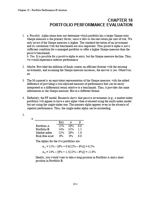
The alphas for the two portfolios are: A = 11% – [6% + 0.8(12% – 6%)] = 0.2% B = 14% – [6% + 1.5(12% – 6%)] = –1.0% Ideally, you would want to take a long position in Portfolio A and a short position in Portfolio B.
11 6 0.5 10
14 6 0.26 31
Therefore, using the Sharpe criterion, Portfolio A is preferred. 6. We first distinguish between timing ability and selection ability. The intercept of the scatter diagram is a measure of stock selection ability. If the manager tends to have a positive excess return even when the market’s performance is merely “neutral” (i.e., the market has zero excess return) then we conclude that the manager has, on average, made good stock picks. In other words, stock selection must be the source of the positive excess returns. Timing ability is indicated by the curvature of the plotted line. Lines that become steeper as you move to the right of the graph show good timing ability. The steeper slope shows that the manager maintained higher portfolio sensitivity to market swings (i.e., a higher beta) in periods when the market performed well. This ability to choose more market-sensitive securities in anticipation of market upturns is the essence of good timing. In contrast, a declining slope as you move to the right indicates that the portfolio was more sensitive to the market when the market performed poorly, and less sensitive to the market when the market performed well. This indicates poor timing. We can therefore classify performance ability for the four managers as follows: A B C D 7. a. Actual: (0.70 2.0%) + (0.20 1.0%) + (0.10 0.5%) = 1.65% Bogey: (0.60 2.5%) + (0.30 1.2%) + (0.10 0.5%) = 1.91% Underperformance = 1.91% – 1.65% = 0.26% Selection Ability Bad Good Good Bad Timing Ability Good Good Bad Bad
- 1、下载文档前请自行甄别文档内容的完整性,平台不提供额外的编辑、内容补充、找答案等附加服务。
- 2、"仅部分预览"的文档,不可在线预览部分如存在完整性等问题,可反馈申请退款(可完整预览的文档不适用该条件!)。
- 3、如文档侵犯您的权益,请联系客服反馈,我们会尽快为您处理(人工客服工作时间:9:00-18:30)。
Chapter 04
Mutual Funds and Other Investment Companies
Mutual funds offer many benefits Some of those benefits include the ability to invest with small amounts of money diversification professional management low transaction costs tax benefits and reduce administrative functions
Close-end funds trade on the open market and are thus subject to market pricing Open-end funds are sold by the mutual fund and must reflect the NAV of the investments
Annual fees charged by a mutual fund to pay for marketing and distribution costs
A unit investment trust is an unmanaged mutual fund Its portfolio is fixed and does not change due to asset trades as does a close-end fund Exchange-traded funds can be traded during the day just as the stocks they represent They are most tax effective in that they do not have as many distributions They also have much lower transaction costs They also
do not require load charges management fees and minimum investment amounts Hedge funds have much less regulation since they are part of private partnerships and free from mist SEC regulation They permit investors to take on many risks unavailable to mutual funds Hedge funds however may require higher fees and provide less transparency to investors This offers
significant counter party risk and hedge fund investors need to be more careful about the firm the invest with
An open-end fund will have higher fees since they are actively marketing and managing their investor base The fund is always looking for new investors A unit investment trust need not spend too much time on such matters since investors find each other
Asset allocation funds may dramatically vary the proportions allocated to each market in accord with the portfolio managers forecast of the relative performance of each sector Hence these funds are engaged in market timing and are not designed to be low-risk investment vehicles
a A unit investment trusts offer low costs and stable portfolios Since they do not change their portfolio the investor knows exactly what they own They are better suited to sophisticated investors
b Open-end mutual funds offer higher levels of service to investors The investors do not have any administrative burdens and their money is actively managed This is better suited for less knowledgeable investors
c Individual securities offer the most sophisticate
d investors ultimat
e flexibility They are able to save money since they are only charged the expenses they incur All decisions are under the control o
f the investor
Open-end funds must honor redemptions and receive deposits from investors This flow of money necessitates retaining cash Close-end funds
no longer take and receive money from investors As such they are free to be fully invested at all times
The offering price includes a 6 front-end load or sales commission meaning that every dollar paid results in only 094 going toward purchase of shares Therefore
Offering price 1138
NAV offering price 1 – load 1230 95 1169
HW
Value of stocks sold and replaced 15000000
Turnover rate 0357 357
NAV 3940
Premium or discount –0086 -86
The fund sells at an 86 discount from NAV
Rate of return 00880 880
HW
Assume a hypothetical investment of 100
Loaded up
a Year 1 100 x 106-0175 10425
b Year 3 100 x 106-0175 3 11630
c Year 10 100 x 106-0175 10 15162
Economy fund
a Year 1 100 x 98 x 106-0025 10364
b Year 3 100 x 98 x 106-0025 3 11590
c Year 10 100 x 98 x 106-0025 10 17141
NAV
a 450000000 – 10000000 44000000 10 per share
b 440000000 – 10000000 43000000 10 per share
Empirical research indicates that past performance of mutual funds is not highly predictive of future performance especially for better-performing funds While there may be some tendency for the fund to be an above ave。