ansys fluent中文版流体计算工程案例详解

合集下载

ansys fluent中文版流体计算工程案例详解

ansys fluent中文版流体计算工程案例详解ANSYS Fluent是一种流体计算动力学软件，可用于解决各种流体力学问题。

本文将详细介绍ANSYS Fluent中文版的流体计算工程案例，包括案例的基本背景、模拟过程和结果分析。

这些案例旨在帮助用户深入了解ANSYS Fluent的使用方法和流体计算工程实践。

一个典型的案例是流体在管道中的流动。

该案例背景是，一根长直管道内有水流动，管道的直径为0.1米，长度为10米。

水的初始速度为1 m/s，管道的壁面是光滑的，管道两端的压差为100Pa。

现在需要使用ANSYS Fluent模拟该流体流动过程，并进一步分析不同参数对流动的影响。

首先，在ANSYS Fluent中创建一个新的仿真项目，并选择“仿真”模块。

在界面上点击“新建”按钮，在弹出的对话框中填写相应的参数，例如案例名称、计算器类型和尺寸单位。

点击“确定”后，进入模拟设置页面。

首先，需要定义获得流动场稳定解所需的物理模型和求解方法。

在“物理模型”选项卡中，选择“连续相”和“非恒定模型”。

在“湍流模型”中选择某种适合的模型，例如k-ε模型。

在“重力”选项卡中，定义流体的密度和重力加速度。

接下来，在“模型”选项卡中，定义管道的几何和边界条件。

选择“管道”作为流体领域的几何模型，并定义长度、直径和内壁面的润滑系数。

在“边界”选项卡中，定义管道两端的入口和出口条件，例如速度和压力。

将管道两端的压力差设置为100Pa，在入口处设置水的初始速度为1 m/s。

在出口处选择“出流”边界条件。

完成几何和边界条件的定义后，点击“模拟”选项卡进入模拟设置界面。

在“求解控制”中，设置计算时间步长和迭代次数。

选择合适的网格划分方法，并进行网格划分。

点击“网格”选项卡，选择合适的网格类型，并进行网格划分。

在划分网格后，可以使用“导入”按钮导入网格文件，并进行网格优化。

完成设置后，点击“计算”按钮开始进行模拟计算。

在计算过程中，可以实时观察流体场的变化情况，并通过Fluent Post-processing工具进行结果分析。

Ansys Workbench零基础超详细单向流体分析的例子

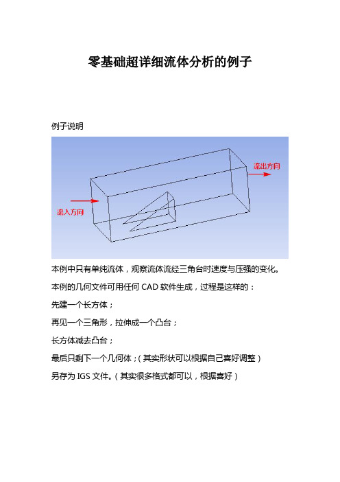
零基础超详细流体分析的例子例子说明本例中只有单纯流体，观察流体流经三角台时速度与压强的变化。

本例的几何文件可用任何CAD软件生成，过程是这样的：先建一个长方体；再见一个三角形，拉伸成一个凸台；长方体减去凸台；最后只剩下一个几何体；（其实形状可以根据自己喜好调整）另存为IGS文件。

（其实很多格式都可以，根据喜好）1.从开始菜单启动WorkBench2.新建mesh cell拖动左边Mesh图标到Schematic中即可3.关联几何文件本例的几何文件是由CatiaV5另存的IGS格式，也可以用Ansys自带的DesignModeler制作，那就要点击New Geometry，而不是Import Geometry。

4.启动ICEM在ICEM中做两件事：建3个Named Selection（inlet、outlet、wall）；划分网格。

4.1.创建Named SelectionA．右键进气（液）面，选Create Named Selection，命名为inletB．同理，选中对面的出气（液）面，命名为outletC．同理，选中剩余8个面，命名为wall。

按住Ctrl键实现多选。

4.2.划分网格A．点击Mesh调出网格划分选项B．展开Sizing，选Relevance Center为Fine，意思是网格划分较细C．另外，做如下设置D．点击Update，生成网格E．保存F．关闭ICEM，回到WB 5.建立一个CFX cell6.Update CFX Cell7.进入CFX-Pre7.1.进入快速设置7.2.设置好一页后点击Next7.3.刷新并保存，退出CFX-Pre8.求解8.1.进入求解器8.2.直接运行8.3.退出求解器9.查看结果9.1.进入后处理器9.2.新建一个观察平面点击apply查看结果点击Apply查看结果。

ANSYS流体第4章flotran流体分析典型工程实例

第4 章FLOTRAN流体分析典型工程实例ANSYS程序中的FLOTRAN CFD流体分析是一个用于分析二维及三维流体流动场的先进工具。

本章重点通过实例讲解介绍FLOTRAN CFD流体分析在工程上的一些典型应用。

本章要点如何解决流体力学问题FLOTRAN流体分析典型工程实例本章案例三维U型管道速度场的数值模拟实际生活中射流现象的数值模拟4.1 如何解决流体力学问题在流体力学的研究中，常用的方法有理论研究方法、数值计算方法和实验研究方法。

理论研究方法的特点是：能够清晰、普遍地揭示出流动的内在规律，但该方法目前只局限于少数比较简单的理论模型。

研究更复杂更符合实际的流动一般采用数值计算方法，它的特点就是能够解决理论研究方法无法解决的复杂流动问题，如常见的航空工程、气象预报、水利工程、环境污染预报、星云演化过程等。

实验研究方法的特点就是结果可靠，但其局限性在于相似准侧不能全部满足、尺寸限制、边界影响等。

数值计算方法和实验研究方法相比，它所需的费用和时间都比较少，并且有较高的精度，但它要求对问题的物理特性有足够的了解（通过实验方法了解），并能建立较精确的描述方程组（通过理论分析）。

对于流体力学的数值模拟常采用的步骤如下。

（1）建立力学模型通过流动分析，采用合理的假设与简化，建立力学模型。

假设与简化：连续介质与不连续介质；理想流体与粘性流体；不可压缩流体与可压缩流体；定常流动与非定常流动。

（2）建立数学模型根据力学模型，建立描述力学模型的数学方程组，并利用无量钢化、量纲分析、引进新的物理参数、经验或半经验公式等方法对基本方程组进行简化，得到相应流动的求解方程组，再根据具体的流动条件确定流动的初始条件和边界条件。

描写流体运动的两种方法：拉格朗日方法和欧拉方法。

（3）求解方法●准确解法：解析解●近似解法：近似解、数值解●实验解法：相似解（4）求解结果速度分布、压力分布、合力、阻力、能量耗散等物理量的求解结果。

ANSYS_CFD之Flotran中文讲解说明

第三步：生成有限元网格
用户必须事先确定流场中哪个地方流体的梯度变化较大，在这些地方，网格必须作适当的调整。例如：如果用了紊流模型，靠近壁面的区域的网格密度必须比层流模型密得多，如果太粗，该网格就不能在求解中捕捉到由于巨大的变化梯度对流动造成的显著影响，相反，那些长边与低梯度方向一致的单元可以有很大的长宽比。为了得到精确的结果，应使用映射网格划分，因其能在边界上更好地保持恒定的网格特性，映射网格划分可由命令 MSHKEY,1 或其相应的菜单 Main Menu>Preproce ssor > -Meshing-Mesh>-entity-Mapped 来实现。
FLUID141 单元
FLUID141 单元具有下列特征：维数：二维形状：四节点四边形或三节点三角形自由度：速度、压力、温度、紊流动能、紊流能量耗散、多达六种流体的各自质量所占的份额
FLUID142 单元
FLUID142 单元具有下列特征：维数：三维形状：四节点四面体或八节点六面体自由度：速度、压力、温度、紊流动能、紊流能量耗散、多达六种流体的各自质量所占的份额
FLOTRAN 分析的主要步骤
一个典型的 FLOTRAN 分析有如下七个主要步骤： 1. 确定问题的区域。 2. 确定流体的状态。 3. 生成有限元网格。 4. 施加边界条件。 5. 设置 FLOTRAN 分析参数。 6. 求解。 7. 检查结果。
第一步：确定问题的区域
用户必须确定所分析问题的明确的范围，将问题的边界设置在条件已知的地方，如果并不知道精确的边界条件而必须作假定时，就不要将分析的边界设在靠近感兴趣区域的地方，也不要将边界设在求解变量变化梯度大的地方。有时，也许用户并不知道自己的问题中哪个地方梯度变化最大，这就要先作一个试探性的分析，然后再根据结果来修改分析区域。这些在后面章节中都有详述。

fluent流体工程仿真计算实例与应用

fluent流体工程仿真计算实例与应用引言流体力学在工程和科学领域中扮演着重要的角色。

通过流体力学的研究，我们可以了解和预测液体和气体在不同条件下的行为。

然而，在真实的实验中，获取流体的准确和详细的数据是非常困难和昂贵的。

因此，流体工程仿真计算成为了一种重要的工具，它可以在实际实验之前通过计算的方式对流体进行建模和分析。

fluent流体工程仿真计算简介Fluent是一款商业化的流体动力学仿真软件，由ANSYS公司开发。

它是一个基于计算流体力学（CFD）的软件工具，能够对各种复杂的流体问题进行建模和分析。

该软件提供了丰富的功能和工具，使工程师能够模拟和解决涉及流体力学的问题。

流体力学仿真计算的优势与传统的实验方法相比，流体力学仿真计算具有以下几个优势： 1. 成本效益：流体力学仿真计算可以节约大量的实验成本，同时缩短了实验周期。

2. 控制参数的灵活性：在真实实验中，很多参数无法被精确控制，而在仿真计算中，我们可以精确地控制和调整各种参数。

3. 快速修改和优化：在实验中，修改和优化系统需要经历繁琐的实验过程，而在仿真计算中，可以轻松地进行快速修改和优化。

4. 可视化和详细分析：通过仿真计算，我们可以获得流体行为的详细信息，同时可以使用可视化工具展示仿真结果。

实例与应用1. 空气动力学仿真空气动力学是流体力学的一个重要分支，研究涉及空气流动的物体。

通过Fluent软件，我们可以对飞行器、汽车、建筑物等在空气中的流动行为进行仿真。

这样的仿真可以帮助工程师改进设计，提高性能和效率。

在空气动力学仿真中，我们可以通过设置不同的参数和条件，如飞行速度、角度、流体密度等，来模拟不同的飞行状态和环境。

通过仿真结果，可以获得飞行过程中的压力分布、升力和阻力等关键性能指标。

2. 建筑气流仿真在建筑领域中，气流对于建筑物的设计和能源消耗具有重要影响。

通过Fluent软件，可以对建筑物内、外的气流进行仿真。

建筑气流仿真可以帮助工程师优化建筑物的通风系统、改善空气质量、减少能耗。

ANSYS CFD管道流体分析经典算例 Fluid

Fluid #2: Velocity analysis of fluid flow in a channel USING FLOTRAN Introduction:In this example you will model fluid flow in a channelPhysical Problem:Compute and plot the velocity distribution within the elbow. Assume that the flow is uniform at both the inlet and the outlet sections and that the elbow has uniform depth.Problem Description:T he channel has dimensions as shown in the figureThe flow velocity as the inlet is 10 cm/sUse the continuity equation to compute the flow velocity at exitObjective:T o plot the velocity profile in the channelT o plot the velocity profile across the elbowYou are required to hand in print outs for the aboveFigure:IMPORTANT: Convert all dimensions and forces into SI unitsSTARTING ANSYSC lick on ANSYS 6.1in the programs menu.S elect Interactive.T he following menu comes up. Enter the working directory. All your files will be stored in this directory. Also under UseDefault Memory Model make sure the values 64 for Total Workspace, and 32 for Database are entered. To change these values unclick Use Default Memory ModelMODELING THE STRUCTUREG o to the ANSYS Utility Menu (the top bar)Click Workplane>W P Settings…The following window comes up:o Check the Cartesian and Grid Only buttonso Enter the values shown in the figure aboveGo to the ANSYS Main Menu (on the left hand side of the screen) and click Preprocessor>Modeling>Create>Keypoints>On Working PlaneCreate keypoints corresponding to the vertices in the figure. The keypoints look like below.Now create lines joining these key points.M odeling>Create>Lines>Lines>Straight lineT he model looks like the one below.Now create fillets between lines L4-L5 and L1-L2.C lick Modeling>Create>Lines>Line Fillet. A pop-up window will now appear. Select lines 4 and 5. Click OK. The following window will appear:T his window assigns the fillet radius. Set this value to 0.1 m.Repeat this process of filleting for Lines 1 and 2.The model should look like this now:N ow make an area enclosed by these lines.M odeling>Create>Areas>Arbitrary>By LinesS elect all the lines and click OK. The model looks like the followingT he modeling of the problem is done.ELEMENT PROPERTIESSELECTING ELEMENT TYPE:Click Preprocessor>Element Type>Add/Edit/Delete... In the 'Element Types' window that opens click on Add... The following window opens.∙Type 1 in the Element type reference number.∙Click on Flotran CFD and select 2D Flotran 141. Click OK. Close the Element types window.∙So now we have selected Element type 1 to be solved using Flotran, the computational fluid dynamics portion of ANSYS. This finishes the selection of element type.DEFINE THE FLUID PROPERTIES:∙Go to Preprocessor>Flotran Set Up>Fluid Properties.∙On the box, shown below, set the first two input fields as Air-SI, and then click on OK. Another box will appear. Accept the default values by clicking OK.∙Now we’re ready to define the Material PropertiesMATERIAL PROPERTIESW e will model the fluid flow problem as a thermal conduction problem. The flow corresponds to heat flux, pressurecorresponds to temperature difference and permeability corresponds to conductance.Go to the ANSYS Main MenuClick Preprocessor>Material Props>Material Models. The following window will appearA s displayed, choose CFD>Density. The following window appears.F ill in 1.23 to set the density of Air. Click OK.Now choose CFD>Viscosity. The following window appears:N ow the Material 1 has the properties defined in the above table so the Material Models window may be closed.MESHING: DIVIDING THE CHANNEL INTO ELEMENTS:G o to Preprocessor>Meshing>Size Cntrls>ManualSize>Lines>All Lines.I n the window that comes up type 0.01 in the field for 'Element edge length'.N ow Click OK.Now go to Preprocessor>Meshing>Mesh>Areas>Free. Click the area and the OK. The mesh will look like thefollowing.BOUNDARY CONDITIONS AND CONSTRAINTSG o to Preprocessor>Loads>Define Loads>Apply>Fluid CFD>Velocity>On lines. Pick the left edge of theouter block and Click OK. The following window comes up.E nter 0.1 in the VX value field and click OK. The 0.1 corresponds to the velocity of 0.1 meter per second of air flowingfrom the left side.R epeat the above and set the Velocity to ZERO for the air along all of the edges of the pipe. (VX=VY=0 for all sides)O nce they have been applied, the pipe will look like this:∙Go to Main Menu>Preprocessor>Loads>Define Loads>Apply>Fluid CFD>Pressure DOF>On Lines.∙Pick the outlet line. (The horizontal line at the top of the area) Click OK.∙Enter 0 for the Pressure value.∙Now the Modeling of the problem is done.SOLUTIONG o to ANSYS Main Menu>Solution>Flotran Set Up>Execution Ctrl.∙The following window appears. Change the first input field value to 300, as shown. No other changes are needed. Click OK.G o to Solution>Run FLOTRAN.W ait for ANSYS to solve the problem.C lick on OK and close the 'Information' window.POST-PROCESSINGP lotting the velocity distribution…Go to General Postproc>Read Results>Last Set.Then go to General Postproc>Plot Results>Contour Plot>Nodal Solution. The following window appears:∙Select DOF Solution and Velocity VSUM and Click OK.∙This is what the solution should look like:∙Next, go to Main Menu>General Postproc>Plot Results>Vector Plot>Predefined.The following window will appear:∙Select OK to accept the defaults. This will display the vector plot to compare to the solution of the same tutorial solved using the Heat Flux analogy. Note: This analysis is FAR more precise as shown by the followingsolution:∙Go to Main Menu>General Postproc>Path Operations>Define Path>By Nodes∙Pick points at the ends of the elbow as shown. We will graph the velocity distribution along the line joiningthese two points.∙The following window comes up.∙Enter the values as shown.∙Now go to Main Menu>General Postproc>Path Operations>Map onto Path. The following window comes up.∙Now go to Main Menu>General Postproc>Path Operations>Plot Path Items>On Graph.∙The following window comes up.∙Select VELOCITY and click OK.∙The graph will look as follows:。

ansys-cfd流体分析实例

ansys-cfd流体分析实例Example on using commercial software“ICEM CFD 5.1”Flow around a circular cylinderY.F.Lin23Two Dimensional problemsFlow around a circular cylinderProblem DescriptionAir flows across a cylinder with the uniform velocity 0.003m/s in the wind tunnel. The length of the wind tunnel (fluid domain) has 25m long and 10 m height. The diameter of cylinder is 1m .Assumption and Boundary Conditions: 1. 2 dimensional problems 2. Steady state condition 3. The uniform flow velocity 4. No Heat transfer5. Neglect the gravitational force6. Constant air densityPre-processing stageIn this stage, we implement the “ICEM CFD” to perform the pre-processing work. The basic steps as follow:1. Establish geometry model2. Block the parts3. Generation the O grid4. Mesh the model and check quality of mesh5. Extrude the mesh6. Reset the BC’s (boundary conditions)7. Output to CFX5.7.1Creating Geometry1. Open ICEM CFDDouble Click the “ICEM CFD” Icon , afterwards, you can see the interface of the ICEMCFD.InOut5DCylinde WallFluid5D20WallOpen File>New Project…:45Set the name with “cylinder_2d”, and Click “Save”2. Creating Geometry: A. PointsClick button “Create Point” and then click button “Explicit Coordinates”Set the points in Cartesian coordinate system(X, Y, Z) with ( X=0, Y=0, Z=0 ) respectively.Click “Apply” button and see the screen: a point is createdA tree widget can be seen at left of the screen (A) and (B)A BThe same method creates other points:X=0; Y=0.5, -0.5 X=-5; Y=5, -5X=20; Y=5, -5 Y=0; X=0.5,-0.567B. Draw line (curve)First of all see the tree widget, open Model>Geometry>Points by right buttonSelect Show Point Names and you can see the name of each point like the figure showed.Now you can create curvesClick button “Create/Modify Curve ”Click button “Create Curve”Note: the left corner of the black screen: Select locationswith left button, middle=done, right=cancelSelect points by using left button of the mouse.Change the name of the Part with “INLET”:8Select PONITS.05 and POINTS.06 with left button (A),And draw a line with middle button “done” (B) and the INLET part is created in the tree widget. The same steps draw the curves named “OUTLET, SIDEA, SIDEB” with the POINTS.07and POINTS.08, POINTS.06 and POINTS.07, POINTS.05 and POINTS.08 respectively.We will see the line and the tree widgetA B910Draw the cylinderClick button “Circle or arc from Center point a nd 2 points on plane”.Set the Part with name “CYLINDER”Click button and select points “POINTS.00,POINTS.01, POINTS.03” with left button respectively (A).A BDraw the cylinder by middle button (B).See tree widget:Close Points name Use button to fit the window.Set the body and material.Click button “Create Body”Choose button “Material Point”and select “Selected surfaces” in the “By Topology” menu. Change the name of the part with “FLUID”; open the Show Point Name of the tree widget and useselect POINTS.06 and POINTS.08.The same way change the part name with “CYLINDER” and select POINTS.01 and POINTS.02. Close Show Point Name and open the tree widget:Open the bodies and you can seeAt last, open the File>Geometry>Save Geometry As…Give it the name with “cylinder_2d”. Click “save”.Now we begin to block the model.Click button “Create Block”See the first one , choose the part with “FLUID”,from the pull down menu select “FLUID”And set the Initialize Blocks type with “2D Planar”Click “Apply” button.A BWe will see that the colors of figure are changed. From (A) to (B)See the tree widget: Model>BlockingThen create some assistant points with button “CreatePoint”{Y=0X=-0.45,-0.4,-0.35,-0.3,-0.25,-0.2,-0.15,-0.1,-0.5, 0.5, 0.1,0.15, 0.2, 0.25, 0.3, 0.35, 0.4, 0.45}{X=0Y=-0.45,-0.4,-0.35,-0.3,-0.25,-0.2,-0.15,-0.1,-0.5, 0.5, 0.1,0.15, 0.2, 0.25, 0.3, 0.35, 0.4, 0.45}Now begin to block the regionClick button “Split Block”Then select button “Split Block”See the split method, select “Prescribed point”Use the put down menu to select the Prescribed point,Use the button firstly select the Edge “INLET”and secondly select the Point “POINTS.03”.We will see the block line in the vertical direction of theINLET.Zoom the fiure.The same way we draw other block lines. From the “POINTS.01 to POINTS.04”See the tree widgetSelect the “Blocking” and select “Index Control”Model>Blocking: Index Control (using right button of the mouse) We can see at the right corner of the screenBy using button and we set I min=2 and see the figureThe same way we set I max =3 , J min=2 , J max=3 And the screen shown thatThe same way block again from “POINTS.00, POINTS.09 to POINTS.44”:(A)(B)(C)After block.See the tree widget: Model>Parts>VORFN :using the right button select “Add to Part”. Click button “Blocking Material”, Add Blocks to PartUsing select blocking regions and we can see Zoom the block regions (A).A B CSelect the blocks in the cylinder or attached the cylinder (B)(C).Using the middle button to set it OK, and you can see blow (D).Click button “Associate”ABDCSelect the associate edge to curve “Associate Edge toCurve”buttonUsing the choose the edge and curveChoosing edge:Select curves:Set O grid CBAClick button “Split Block”Click “Ogird Block”buttonSelect theSee the tree widget: Open Model>Parts>VORFNOpen the VORFN (A)AUsing button to selectin or attached the cylinder (B)(C)(D).B CD EUsing middle button to click “Apply” (E)Close “VORFN” from the tree widget (F)F GClick the “Reset”(G) Mesh the edgesClick button “Set Curve Mesh Size”Using button to select Curve(s):Choose Method with “Element count”Set the Number with 100 and click Apply.See the tree: close the Model>Geometry>points, and the Model>Blocking>edgesUsing right button to select Model>Geometry>Curves:Curve Node Spacing (by using right button)The same way set the “INLET” and “OUTLET” with number 100, the “SIDEA” and “SIDEB”with number 250.Click button “Pre-Mesh Params”Choose Blocking >Pre-Mesh ParamsClick button “Update Sizes”and keep default,Then click ApplySee tree open Model>Blocking>Pre_Mesh: Project faces(by using right button)And we will see a menuClick Yes.Now we will see the mesh of the model.Zoom it see the local partClose Geomery>Points and curves, and Blocking>Edges.Then open File>Mesh>Load from BlockingOpen File>Mesh>Save Mesh As…: and set the name with “cylinder_2d”Open File>Blocking>Save Blocking As…: Save block with the name “cylinder_2d”Check the quality of the meshClick button “Display Mesh Quality”Click ApplyWe can see no negatives mesh.Extrude meshClick button “Extrude Mesh”Use to select Elements:Method 1Click button “Select items in a part”and a menu appears:Click “All” and “Accept”Method 2A BPut the left button and drag it to select all the regions (A)(C). Click middle button to accept (B) Give the New volume part name “FLUID2D”, new side part name “SIDE”, new top par name “TOP”And set the Spacing type>spacing with “0.1”, then ApplyCSo the mesh change a height 0.1 in the Z direction (D)DBox ZoomE FClick button “Shaded Full Display”(E)(F) Check the quality of the extrude meshSee the tree widget:Close top “TOP” (B) Close “FLUID” (C) A BSet the new boundary conditionsSee the tree widget:Model>Parts: Create Part (by using the right button)Click “Create Part by Selection” button From the pull down menu of the Part: select the “CYLINDER” Using and left button drag the regionUsing middle button accepts it, so a new CYLINDER boundary condition has been set (C).CBACThe same way set the INLET, OUTLET, SIDEA and SIDEB boundary conditions. INLETThe Whole Boundary Conditions CA BSee the tree widget:A Open Model>Parts>FLUID(B)B Open Model>Parts>TOP(C)CSix kinds of patternsClick File>Mesh>Save Mesh As…And save the new mesh with name “cylinder_2d_extrude”. Output the mesh file to CFXClick button “Select solver”and choose “CFX-5”Click “Okay”CBFEDAClick button “Write input”Keep default and click “Done”Then the Domain selection appearsKeep the Selected domains with “cylinder_2d_extrude.uns” and click “Done”.Now we will see the created files in working directions:From these files, we must note that only the file named “cfx5” can be inputted into CFX5.7.1 The mesh is finished.Other examples:Example on using commercial software“CFX 5.7.1”Flow around a circular cylinderY.F.LinTwo Dimensional problemsFlow around a circular cylinderAfter established the geometry model, we begin to use CFX to solve this two dimensional case. Processing with CFX-5.7.11.Open CFXDouble click the “CFX” Icon, afterwards, you can see the interface of the CFX.There are three kinds of functions of the CFX:1.CFX-Pre 5.7.1 (set the relevant parameters).2.CFX-Solver 5.7.1 (solve the case by using established physical model)3.CFX-Post 5.7.1 (get the data and figures which we need)CFX-Pre step:1.Import the mesh file from ICEM CFD2.Simulation type3.Domain4.BC’s (boundary conditions)5.Initial conditions6.Solver control7.Output file and monitor points8.Write “.def” file and simulationClick button “CFX-Pre 5.7.1”and run it.Establish a new simulationOpen File>New Simulation…:Select button “General”and give the file namewith “cylinder_2d”. Click “Save”Now we can see the interface of the CFX-PreImport mesh fileSee the middle position of the screen, Click button “Import mesh”Open Mesh>Definition>Mesh Format:From the pull down menu select “ICEM CFD”, (see figure below)Definition>File: Click button “Browse”Find the working direction and select the file named “cfx5”,Then click “Open” button. And “OK”Note: no other files can be inputted in CFX5.7.1Then the mesh file has been inputted into the CFX-PreAnd the left window appears.All of these names were already defined by us in “ICEM CFD”Set the relevant parameters1. Define the simulation type:Click button “Define the Simulation Type”button.Note: the blue color note suggest we should set a domain. Then the simulation type appearsBasic Settings>Option: Select “Transient”Basic Settings>Time Duration>Option: From the pull down menu select Total Time.Basic Settings>Time Duration>Total Time: Set with 42000s.Basic Settings>Time Steps>Option: From the pull down menu select Timesteps.Basic Settings>Time Steps>Timesteps: Set with 1s.Initial Time>Option: From the pull down menu select Autorratic.Then click Apply and Ok2. Create a domain:Click button “Create a Domain”.Set the name with “ cylinder2d” and click OkSee figure below: the color of the domain changed into green, and the window “Edit Domain”appears.General Options>Basic Settings>Location: From the pull down menu select “FLUID2D”Then click “Apply” buttonFluid Models>Heat Transfer Model>Option:Keep by default.Fluid Models>Heat Transfer Model>FluidTemperature: Set the temperature with 25c.Fluid Models>Turbulence Model>Option: Setit with “None(Laminar).Click OK3. Set boundary condtions:Click button “Create a Boundary Condition”Set INLET boundary conditionSet the Name with “INLET” and click OK。

ansys fluent中文版流体计算工程案例详解