第十二章 分层回归分析--Hierarchy Regression
回归分析(regression analysis)
回归分析(regression analysis)➢概述回归分析是寻求成对出现的一组数值型数据之间的关系模型的一种统计工具,这咱关系模型是一条直线或曲线。
回归分析就是要找到这条直线或曲线的方程,以及度量模型对数据拟合优度的判定系数r2和其他一些统计工具。
线性回归是通过绘制数据的散布图来拟合一条最优直线。
本部分将就这种最简单的回归类型展开讨沦。
非线性回归是寻求与数据最优的曲线。
多元回归是解决一个因变量受多个自变量影响的问题。
非线性和多元回归都过于复杂,需要使用时可以寻求统计学家的帮助。
➢适用场合·当取得一组成对出现的数据型数据时;·在绘制完成数据的散布图后;·当要了解自变量的变化对因变量有怎样的影响时;·当掌握了自变量的信息,想要预测因变量的变化情况时;·当需要得到直线或曲线对数据的拟合程度的统汁测量结果时。
➢实施步骤线性回归可以用手工完成,但是通过计算机软件可以大大简化运算。
按照软件说明逐步完成分析过程。
回归分析会得到与数据最优拟合的回归直线图形以及一张统计表格,包括:·回归直线的斜率。
直线方程的形式是:ˆy mx b=+,m是斜率,代表当自变量x增加一个单位时,因变量ˆy将随之增加一个单位。
正的斜率意味着回归线是由左向右上方倾斜的;负斜率说明回归线向下方倾斜(ˆy的上标是用来提醒它只是因变量)估计值,而不是真实值)。
·回归直线的截距。
在直绒方程中,常数b代表截距。
它是直线与y轴交点处ˆy的值。
得到斜率和截距值后,就可以根据等式ˆy mx b=+画出回归线或按照给定的x值估计y的值了。
·判定系数r2。
r2的值介于0和1之间,是对同归线与数据拟合程度的度量。
如果,r2=1,代表直线与数据完全吻合。
随着r2值的减小,表示拟合度越差,得到的估计值也更不准确。
将r2看作是y的变动中可以用回归直线解释的那部分,因为大部分的数据点都不会准确地落在回归线上,不能用回归线解释的那部分(1—r2)是残差。
hierarchical regression analysis
hierarchical regression analysis 层次回归分析是一种广泛应用于社会科学、心理学和教育研究的统计方法。
它是一种多元线性回归分析的变体,它允许考虑不同层次的变量对因变量的影响。
在本文中,我们将介绍层次回归分析的基本概念、步骤和应用,以及一些常见的数据分析问题和解决方法。
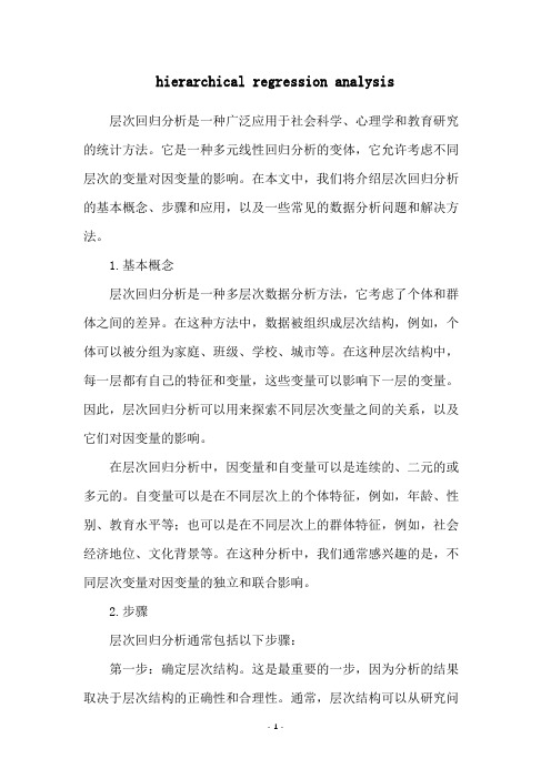
1.基本概念层次回归分析是一种多层次数据分析方法,它考虑了个体和群体之间的差异。
在这种方法中,数据被组织成层次结构,例如,个体可以被分组为家庭、班级、学校、城市等。
在这种层次结构中,每一层都有自己的特征和变量,这些变量可以影响下一层的变量。
因此,层次回归分析可以用来探索不同层次变量之间的关系,以及它们对因变量的影响。
在层次回归分析中,因变量和自变量可以是连续的、二元的或多元的。
自变量可以是在不同层次上的个体特征,例如,年龄、性别、教育水平等;也可以是在不同层次上的群体特征,例如,社会经济地位、文化背景等。
在这种分析中,我们通常感兴趣的是,不同层次变量对因变量的独立和联合影响。
2.步骤层次回归分析通常包括以下步骤:第一步:确定层次结构。
这是最重要的一步,因为分析的结果取决于层次结构的正确性和合理性。
通常,层次结构可以从研究问题、数据来源、理论框架等方面确定。
第二步:确定模型。
在层次回归分析中,有两种基本模型:随机截距模型和随机斜率模型。
随机截距模型假设不同层次的个体之间存在随机差异,但自变量对因变量的影响是相同的。
随机斜率模型假设不同层次的个体之间存在随机差异,并且自变量对因变量的影响也可能因层次而异。
在选择模型时,需要考虑研究问题、数据的特点、理论假设等因素。
第三步:进行模型拟合。
在层次回归分析中,通常使用最大似然估计或贝叶斯方法进行参数估计。
拟合模型时,需要考虑模型的拟合度、参数的显著性、模型的解释力等方面。
第四步:进行模型诊断。
模型诊断是判断模型是否合理和可靠的重要步骤。
常用的方法包括检查残差图、Q-Q图、杠杆点和离群值等。
大学生性别角色与社会适应的关系模型概要
Advances in Social Sciences 社会科学前沿 , 2015, 4(4, 218-224Published Online December 2015 in Hans.文章引用 : 申可 , 陈红 . 大学生性别角色与社会适应的关系模型 [J]. 社会科学前沿 , 2015, 4(4: 218-224.The Relationship between Sex-Role and Social Adaption of College Students Ke Shen, Hong Chen*Department of Psychology, Southwest University, ChongqingReceived: Nov. 1st , 2015; accepted: Nov. 20th , 2015; published: Nov. 23rd , 2015Copyright © 2015 by authors and Hans Publishers Inc.This work is licensed under the Creative Commons Attribution International License (CC BY.AbstractIn western culture, three theories regarding the utility of sex-roles have been proposed: the con-gruency model, the androgyny model, and the masculinity model. The congruency model posits that masculin ity facilitates males’ mental health but not females’, while femininity facilitates fe-males’ well-being but not males’. Androgyny model states that people with high levels of both masculinity and femininity enjoy the highest level of well-being independent of their gender. Masculinity model holds thatmasculinity is the dominant factor that promotes ones’ psychological well-being. This study used Students’ Sex Role Inventory (CSRI-50 and College Students Adapta-bility Scale (CSAI to investigate, random sample of 188 subjects from local universities, to explore the applicability of three models in college students. The results showed that the masculinity model is most appropriate in explaining the relation of sex-role to social adaptation in college students. KeywordsCollege Students, Sex Role, Social Adaption大学生性别角色与社会适应的关系模型申可,陈红 *西南大学心理学部,重庆收稿日期:2015年 11月 1日;录用日期:2015年 11月 20日;发布日期:2015年 11月 23日*通讯作者。
层次分析法介绍

层次分析法介绍我顶!一.层次分析法的基本原理1.引言层次分析法(Analytia1 Hierarchy Process,简称AHP)是美国匹兹堡大学教授A.L.Saaty于20世纪70年代提出的一种系统分析方法。
AHP是一种能将定性分析与定量分析相结合的系统分析方法。
AHP是分析多目标、多准则的复杂大系统的有力工具。
它具有思路清晰、方法简便、适用面广、系统性强等特点,便于普及推广,可成为人们工作和生活中思考问题、解决问题的一种方法。
将AHP引入决策,是决策科学化的一大进步。
它最适宜于解决那些难以完全用定量方法进行分析的决策问题,因此,它是复杂的社会经济系统实现科学决策的有力工具。
应用AHP解决问题的思路是:首先,把要解决的问题分层系列化,即根据问题的性质和要达到的目标,将问题分解为不同的组成因素,按照因素之间的相互影响和隶属关系将其分层聚类组合,形成一个递阶的、有序的层次结构模型。
然后,对模型中每一层次因素的相对重要性,依据人们对客观现实的判断给予定量表示,再利用数学方法确定每一层次全部因素相对重要性次序的权值。
最后,通过综合计算各层因素相对重要性的权值,得到最低层(方案层)相对于最高层(总目标)的相对重要性次序的组合权值,以此作为评价和选择方案的依据。
2.基本原理我们可以分析下面这个简单的例子,来说明AHP的基本原理。
二.层次分析法的步骤用AHP分析问题大体要经过以下五个步骤:(1)建立层次结构模型;(2)构造判断矩阵;(3)层次单排序;(4)层次总排序;(5)一致性检验。
其中后三个步骤在整个过程中需要逐层地进行。
1.建立层次结构模型运用AHP进行系统分析,首先要将所包含的因素分组,每一组作为一个层次,按照最高层、若干有关的中间层和最低层的形式排列起来。
对于决策问题,通常可以将其划分成层次结构模型。
其中:最高层:表示解决问题的目的,即应用AHP所要达到的目标。
中间层:它表示采用某种措施和政策来实现预定目标所涉及的中间环节,一般又分为策略层、约束层、准则层等。
分层回归分析的意义

分层回归分析的意义
1、分层回归分析的意义?
【答案】分层回归(层次回归)本质上是建立在回归分析基础上,区别在于分层回归可分为多层,用于研究两个或者多个回归模型之间的差异。
分层回归将核心研究的变量放在最后一步进入模型,以考察在排除了其他变量的贡献的情况下,该变量对回归方程的贡献。
如果变量仍然有明显的贡献,那么就可以做出该变量确实具有其他变量所不能替代的独特作用的结论。
这种方法主要用于,当自变量之间有较高的相关,其中一个自变量的独特贡献难以确定的情况。
例如,在研究学习疲倦感中,将性别、年龄、学历等(控制变量)放置在第一层,第二层放置工作压力(核心研究变量)。
常用于中介作用或者调节作用研究。
分层回归分析
分层回归分析
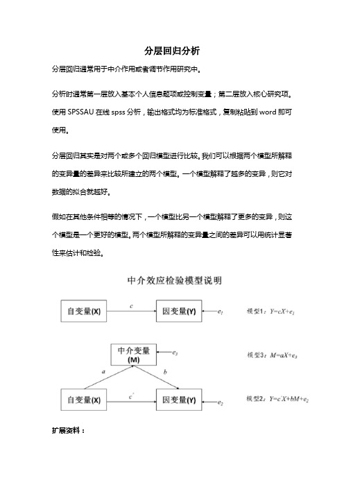
分层回归通常用于中介作用或者调节作用研究中。
分析时通常第一层放入基本个人信息题项或控制变量;第二层放入核心研究项。
使用SPSSAU在线spss分析,输出格式均为标准格式,复制粘贴到word即可使用。
分层回归其实是对两个或多个回归模型进行比较。
我们可以根据两个模型所解释的变异量的差异来比较所建立的两个模型。
一个模型解释了越多的变异,则它对数据的拟合就越好。
假如在其他条件相等的情况下,一个模型比另一个模型解释了更多的变异,则这个模型是一个更好的模型。
两个模型所解释的变异量之间的差异可以用统计显著性来估计和检验。
扩展资料:
前面介绍的回归分析中的自变量和因变量都是数值型变量,如果在回归分析中引入虚拟变量(分类变量),则会使模型的应用范围迅速扩大。
在自变量中引入虚拟变量本身并不影响回归模型的基本假定,因为经典回归分析是在给定自变量X 的条件下被解释变量Y的随机分布。
但是如果因变量为分类变量,则会改变经典回归分析的基本假定,一般在计量经济学教材中有比较深入的介绍,如Logistics回归等。
层次分析法(AHP)简介

系
要
层
矩
权
统
素
次
阵
重
AHP的基本原理
基本原理 AHP决策分析方法的基本原理,可以用以下的简单事例分析来
说明。 假设有n个物体A1,A2,…,An,它们的重量分别记为W1,
W2,…,Wn。现将每个物体的重量两两进行比较如下:
AHP的基本原理
若以矩阵来表示各物体的这种相互重量关系,
W1 / W1 W1 / W2 W1 / Wn
人的技 术素质
经营管 理水平
建立判断矩阵
判断矩阵是以上一级的某一要素C作为评价准则,对本级的要素进 行两两比较来确定矩阵元素的。
例如,以C为评价标准的有n个要素,其判断矩阵形式如下:
C
B1
B2 …
Bj
…
Bn
B1
b11
b12 …
b1j
…
b1n
B2
b21
b22 …
b2j
…
b2n
…
…
…
…
…
…
Bi
bi1
假如上一层的层次总排序已经完成,元素A1,A2,…,Am得到的权重值
分别为a1,a2,…,am;与Aj对应的本层次元素B1,B2,…,Bn的层次单排
序结果为[b1j , b2j ,, bnj 那么,B层次的总排序结果见表。
]T(当Bi与Aj无联系时,bi j =0);
层次总排序表
综合重要度的计算
对层次分析法的简单评价
优点:思路简单明了,它将决策者的思维过程条理化、数量化,便于计算,容易 被人们所接受;
所需要的定量化数据较少,但对问题的本质,问题所涉及的因素及其内在关 系分析得比较透彻、清楚。
Regression回归分析

Regression回归分析Regression Analysis (Spring, 2000)By WonjaePurposes: a. Explaining the relationship between Y and X variables with a model (Explain a variable Y in terms of Xs)b. Estimating and testing the intensity of their relationshipc. Given a fixed x value, we can predict y value.(How does a change of in X affect Y, ceteris paribus?)(By constructing SRF, we can estimate PRF.)OLS (ordinary least squares) method: A method to choose the SRF in such a way that the sum of the residuals is as small as possible.Cf. Think of ‘trigonometrical function’ and ‘the use of differentiation’Steps of regression analysis:1. Determine independent and dependent variables: Stare one dimension function model!2. Look that the assumptions for dependent variables are satisfied: Residuals analysis!a. Linearity(assumption 1)b. Normality (assumption 3)— draw histogram for residuals (dependent variable) or normal P-P plot(Spss statistics regression linear plots ‘Histogram’, ‘Normal P-P plot ofregression standardized’)c. Equal variance (homoscedasticity: assumption 4)—draw scatter plot for residuals (Spss statistics regression linear plots: Y = *ZRESID, X =*ZPRED)Its form should be rectangular!If there were no symmetry form in the scatter plot, we should suspect the linearity.d. Independence (assumption 5,6: no autocorrelation between the disturbances,zero covariance between error term and X)—each individual should be independent3. Look at the correlation between two variables by drawing scatter graph:(Spss graph scatter simple)a. Is there any correlation?b. Is there a linear relation?c. Are there outliers? If yes, clarify the reason and modify it!(We should make outliers dummy as a new variable, and do regression analysis again.)d. Are there separated groups? If yes, it means those data came from different populations4. Obtain a proper model by using statistical packages (SPSS)5. Test the model:a. Test the significance of the model (the significance of slope): F-TestIn the ANOV A table, find the f-value and p-value(sig.)If p-value is smaller than alpha, the model is significant.b. Test the goodness of fit of the model In the ‘Model Summary’, look at R-square. R-square(coefficient of determination)—It measures the proportion or percentage ofthe total variation in Y explained by the regression model. (If the model is significant but R-square is small, it means that observed values arewidely spread around the regression line.)6. Test that the slope is significantly different from zero:a. Look at t-value in the ‘Coefficients’ table and find p-vlaue.b. T-square should be equal to F-value.7. If there is the significance of the model, Show the model and interpret it!steps: a. Show the SRFb. In “Model Summary” Interpret R-square!c. In “ANOV A” table Show the table, interpret F-value and the null hypothesis!d. In “Coefficients” table Show the table and interpret beta values!e. Show the residuals statistics and residuals’ scatter plot!If there is no significance of the model, interpret it like this:“X variable is little helpful for explaining Y variable.” or“There is no linear relationship between X variable and Y variable.”8. Mean estimation (prediction) and individual prediction :We can predict the mean, individuals and their confidence intervals.(Spss statistics regression linear save predicted values: unstandardized)Testing a modelWonjaeBefore setting up a model1. Identify the linear relationship between each independent variable and dependent variable. Create scatter plot for each X and Y.( STATA: plot Y X1, plot Y X2)ovtest, rhsgraph Y X1 X2 X3, matrixavplots)2. Check partial correlation for each X and Y.( STATA: pcorr Y X1 X2, pcorr X1 Y X2, pcorr X2 Y X1 )After setting up a model1. Testing whether two different variables have same coefficients.The null hypothesis is that “X1” and “X2”variables have the same impact on Y.( STATA: test X1 = X2 )2. Testing Multicollinearity (Gujarati, p.345)1) DetectionHigh R2 but few significant t-ratios.High pair-wise (zero-order) correlations among regressors( STATA: regress Y X1 X2 X3graph Y X1 X2 X3, matrixavplots)Examination of partial correlationsAuxiliary regressionsEigen-values and condition indexTolerance and variance inflation factor( STATA: regress Y X1 X2 X3vif)# Interpretation: If a VIF is in excess of 20, or a tolerance (1/VIF) is .05 or less,There might be a problem of multicollinearity.2) Correction:A. Do nothingIf the main purpose of modeling is predicting Y only, then don’t worry.(since ESS is left the same)“Don’t worry about multicollinearity if the R-squared from the regression exceeds the R-squared of any independent variable regressed on the other independent variables.”“Don’t worry about it if the t-statistics are all greater than 2.”(Kennedy, Peter. 1998. A Guide to Econometrics: 187)B. Incorporate additional informationAfter examining correlations between all variables, find the most strongly relatedvariable with the others. And simply omit it.( STATA: corr X1 X2 X3)Be careful of the specification error, unless the true coefficient of that variable is zero.Increase the number of dataFormalize relationships among regressors: for example, create interaction term(s)If it is believed that the multicollinearity arises from an actual approximate linearrelationship among some of the regressors, this relationship could be formalized and the estimation could then proceed in the context of a simultaneous equation estimation problem.Specify a relationship among some parameters: If it is well-known that there exists a specific relationship among some of the parameters in the estimating equation, incorporate this information. The variances of the estimates will reduce.Form a principal component: Form a composite index variable capable of representing this group of variables by itself, only if the variables included in the composite havesome useful combined economic interpretation.Incorporate estimates from other studies: See Kennedy (1998, 188-189).Shrink the OLS estimates: See Kennedy.3. Heteroscedasticity1) DetectionCreate scatter plot for ‘residual squares’ and Y (p.368)Create scatter plot for each X and Y residuals (standardized)(“Partial Regression Plot” in SPSS)( STATA: predict rstanplot X1 rstanplot X2 rstan )White’s test (p.379)Step 1: regress your model (STATA: reg Y X1 X2…)Step 2: obtain the residuals and the squared residuals( STATA: predict resi / gen resi2 = resi^2 )Step 3: generate the fitted values yhat and the squared fitted values yhat( STATA: predict yhat/ gen yhat2 = yhat^2 )Step 4: run the auxiliary regression and get the R2( STATA: reg resi2 yhat yhat2 )Step 5: 1) By using f-statistic and its p-value, evaluate the null hypothesis.or 2) By comparing χ2calculated (n times R2) with χ2critical , evaluate it again.If the calculated value is greater than the critical value (reject the null),there might be ‘heteroscedasticity’ or ‘specification bias’ or both.Cook & Weisberg test( STATA: regress Y X1 X2 X3hettest)The Breusch-Pagan test( STATA: reg Y X1 X2 …. / predict resi / gen resi2 = resi^2 / reg res2 X1 X2…)2) Remedial measureswhen variance is known: use WLS method( STATA: reg Y* X0 X1* noconstant )cf. Y* =Y/δ , X* = X/δwhen variance is not known: use white’ method( STATA: gen X2r =sqrt(X) , gen dX2r =1/X2rgen Y* = Y/X2rreg Y* dX2r X2r, noconstant )4. Autocorrelation1) DetectionCreate plot( STATA: predict resi, resigen lagged resi =resi[_n-1]plot resi lagged resi)Durbin-Watson d test(Run the OLS regression and obtain the residuals compute ‘d’find d Lcritical and d Uvalues, given the N and K decide according to the decision rules)( STATA: regress Y X1 X2 X3dwstat )Runs test( STATA: regress Y X1 X2 X3predict resi, resiruntest resi)2) Remedial measures (pp.426-433)Estimate ρ: ρ = 1 – d/2 (D-W) or ρ = n2(1- d/2) + k2/n2 –k2 (Theil-Nagar)Regress with transformed variables and get the new d statistic.Compare it with d Lcritical and d Uvalues5. Testing Normality of residualsobtain ‘normal probability plot’(With ‘ZY’ and ‘ZX’, choose ‘Normal probability plot’ in SPSS)( STATA: predict resi, resi egen zr =std(resi)pnorm zr )6. Testing OutliersDetection(STATA: avplot x1 / cprplot X1 / rvpplot X1)Cooksd test: Cook’s distance, which measures the aggregate change in the estimated coefficients, when each observation is left out of the estimation(STATA: regress Y X1 X2predict c, cooksddisplay 4/d.f. remember this cut point value!list X1 X2 c compare the values in c with the cut point value!list c if c > 4/d.f. identify which observations are outliers!drop if c > 4/d.f. If you want to drop outliers! )。
- 1、下载文档前请自行甄别文档内容的完整性,平台不提供额外的编辑、内容补充、找答案等附加服务。
- 2、"仅部分预览"的文档,不可在线预览部分如存在完整性等问题,可反馈申请退款(可完整预览的文档不适用该条件!)。
- 3、如文档侵犯您的权益,请联系客服反馈,我们会尽快为您处理(人工客服工作时间:9:00-18:30)。
分层回归其实是对两个或多个回归模型进行比较。
我们可以根据两个模型所解释的变异量的差异来比较所建立的两个模型。
一个模型解释了越多的变异,则它对数据的拟合就越好。
假如在其他条件相等的情况下,一个模型比另一个模型解释了更多的变异,则这个模型是一个更好的模型。
两个模型所解释的变异量之间的差异可以用统计显著性来估计和检验。
模型比较可以用来评估个体预测变量。
检验一个预测变量是否显著的方法是比较两个模型,其中第一个模型不包括这个预测变量,而第二个模型包括该变量。
假如该预测变量解释了显著的额外变异,那第二个模型就显著地解释了比第一个模型更多的变异。
这种观点简单而有力。
但是,要理解这种分析,你必须理解该预测变量所解释的独特变异和总体变异之间的差异。
一个预测变量所解释的总体变异是该预测变量和结果变量之间相关的平方。
它包括该预测变量和结果变量之间的所有关系。
预测变量的独特变异是指在控制了其他变量以后,预测变量对结果变量的影响。
这样,预测变量的独特变异依赖于其他预测变量。
在标准多重回归分析中,可以对独特变异进行检验,每个预测变量的回归系数大小依赖于模型中的其他预测变量。
在标准多重回归分析中,回归系数用来检验每个预测变量所解释的独特变异。
这个独特变异就是偏相关的平方(Squared semi-partial correlation)-sr2(偏确定系数)。
它表示了结果变量中由特定预测变量所单独解释的变异。
正如我们看到的,它依赖于模型中的其他变量。
假如预测变量之间存在重叠,那么它们共有的变异就会削弱独特变异。
预测变量的独特效应指的是去除重叠效应后该预测变量与结果变量的相关。
这样,某个预测变量的特定效应就依赖于模型中的其他预测变量。
标准多重回归的局限性在于不能将重叠(共同)变异归因于模型中的任何一个预测变量。
这就意味着模型中所有预测变量的偏决定系数之和要小于整个模型的决定系数(R2)。
总决定系数包括偏决定系数之和与共同变异。
分层回归提供了一种可以将共同变异分配给特定预测变量的方法。
分层回归标准多重回归可以测量模型所解释的变异量的大小,它由复相关系数的平方(R2,即决定系数)来表示,代表了预测变量所解释的因变量的变异量。
模型的显著性检验是将预测变量所解释的变异与误差变异进行比较(即F值)。
但是,也可以采用相同的方式来比较两个模型。
可以将两个模型所解释的变异之差作为F 值的分子。
假如与误差变异相比,两个模型所解释的变异差别足够大,那么就可以说这种差别达到了统计的显著性。
相应的方程式将在下面详细阐述。
分层回归就是采用的这种方式。
分层回归包括建立一系列模型,处于系列中某个位置的模型将会包括前一模型所没有的额外预测变量。
假如加入模型的额外解释变量对解释分数差异具有显著的额外贡献,那么它将会显著地提高决定系数。
这个模型与标准多重回归的差异在于它可以将共同变异分配到预测变量中。
而在标准多重回归中,共同变异不能分配到任何预测变量中,每个预测变量只能分配到它所解释的独特变异,共同变异则被抛弃了。
在分层回归中,将会把重叠(共同)变异分配给第一个模型中的预测变量。
因此,共同变异将会分配给优先进入模型的变量。
重叠的预测变量(相关的预测变量Predictor variables that overlap)简单地看来,由一系列预测变量所解释的变异就像一块块蛋糕堆积在一起。
每个预测变量都有自己明确的一块。
它们到达桌子的时间是无关紧要的,因为总有同样大小的蛋糕在等着它们。
不同部分变异的简单相加就构成了某个模型所解释的总体变异。
但是,这种加法的观点只有在每个预测变量互相独立的情况下才是正确的。
对于多重回归来说,则往往不正确。
假如预测变量彼此相关,它们就会在解释变异时彼此竞争。
归因于某个预测变量的变异数量还取决于模型中所包含的其他变量。
这就使得我们对两个模型的比较进行解释时,情况变得更为复杂。
方差分析模型是建立在模型中的因素相互独立的基础上的。
在ANOVA中,因素对应于多重回归中的预测变量。
这些因素具有加法效应,变异(方差)可以被整齐地切开或分割。
这些因素之间是正交的。
但是,在多重回归中,变量进入模型的顺序会影响该变量所分配的变异量。
在这种情况下,预测变量就像一块块浸在咖啡杯中的海绵。
每一块都吸收了一些变异。
在分层多重回归中,第一块浸入咖啡杯的海绵首先吸收变异,它贪婪地吸收尽可能多的变异。
假如两个预测变量相关,那它们所解释的变异就存在重叠。
如果一个变量首先进入模型,那它就将重叠(共同)变异吸收据为己有,不再与另一个变量分享。
在标准多重回归中,所有预测变量同时进入模型,就像将所有海绵同时扔进咖啡杯一样,它们互相分享共同变异。
在这种情况下,偏相关的平方(sr2)与回归系数相等,它们检验了相同的东西:排除了任何共同变异后的独特变异。
这样,在多重回归中,对回归系数的T 检验就是sr2的统计显著性检验。
但是,在分层回归或逐步回归中,sr2不再与回归系数相等。
但T检验仍然是对回归系数的检验。
要估计sr2是否显著,必须对模型进行比较。
模型比较就是首先建立一个模型(模型a),使它包括除了要检验的变量以外的所有变量,然后再将想要检验的变量加入模型(模型b),看所解释的变异是否显著提高。
要检验模型b 是否要比模型a显著地解释了更多的变异,就要考察各个模型所解释的变异之差是否显著大于误差变异。
下面就是检验方程式(Tabachnik and Fidell, 1989)。
(R2b-R2a)/MF = ————————(1+ R2b) /dferror(2为平方,a,b为下标。
不知道在blog里如何设置文字格式)原文(DATA ANALYSIS FOR PSYCHOLOGY, George Dunbar)如此,但参考了其他书后,觉得这是误印,真正的公式应该是这样的:(R2b-R2a)/MF = ————————(1- R2b) /dferror注:M是指模型b中添加的预测变量数量R2b是指模型b(包含更多预测变量的模型)的复相关系数的平方(决定系数)。
R2a是指模型a(包含较少预测变量的模型)的复相关系数的平方(决定系数)。
dferror是指模型b误差变异的自由度。
分层回归与向前回归、向后回归和逐步回归的区别后三者都是选择变量的方法。
向前回归:根据自变量对因变量的贡献率,首先选择一个贡献率最大的自变量进入,一次只加入一个进入模型。
然后,再选择另一个最好的加入模型,直至选择所有符合标准者全部进入回归。
向后回归:将自变量一次纳入回归,然后根据标准删除一个最不显著者,再做一次回归判断其余变量的取舍,直至保留者都达到要求。
逐步回归是向前回归法和向后回归法的结合。
首先按自变量对因变量的贡献率进行排序,按照从大到小的顺序选择进入模型的变量。
每将一个变量加入模型,就要对模型中的每个变量进行检验,剔除不显著的变量,然后再对留在模型中的变量进行检验。
直到没有变量可以纳入,也没有变量可以剔除为止。
向前回归、向后回归和逐步回归都要按照一定判断标准执行。
即在将自变量加入或删除模型时,要进行偏F检验,计算公式为:(R2b-R2a)/MF = ————————(1- R2b) /dferrorSPSS回归所设定的默认标准是选择进入者时偏F检验值为3.84,选择删除者时的F检验值为2.71。
从上面可以看出,分层回归和各种选择自变量的方法,其实都涉及模型之间的比较问题,而且F检验的公式也相等,说明它们拥有相同的统计学基础。
但是,它们又是不同范畴的概念。
分层回归是对于模型比较而言的,而上面三种方法则是针对自变量而言的。
上面三种选择自变量的方法,都是由软件根据设定标准来自动选择进入模型的变量。
而分层回归则是由研究者根据经验和理论思考来将自变量分成不同的组(block),然后再安排每一组变量进入模型的顺序,进入的顺序不是根据贡献率,而是根据相应的理论假设。
而且,研究者还可以为不同组的自变量选用不同的纳入变量的方法。
分层回归在SPSS上的实现在线性回归主对话框中,在定义完一组自变量后,在因变量不变的情况下,利用block前后的previous和next按钮,继续将其他变量组加入模型。
我所设计的回归模型中,有a自变量,b为调节变量,a与b的交互项,4个控制变量,1个因变量。
我打算用分层回归模型来做。
(我主要为验证自变量a以及b调节作用)第一步,在"Block of 1 " 中,我将4个控制引入到"Independent"中,"Method "选择"Enter",然后点击NEXT。
第二步,在“Block of 2"中,将a,b及交互项引入”Independent"中,“Mehod" 选择”stepwise”。
我想问各位大咔,我这样做对吗?还有,分层回归和逐步回归有什么区别?我是否可以将第二步省略,直接把a,b,交互项放入Block of 1 中,Method变为sterwise?。