机器学习决策树 ID3算法的源代码

合集下载

决策树之ID3算法

决策树之ID3算法⼀、决策树之ID3算法简述 1976年-1986年，J.R.Quinlan给出ID3算法原型并进⾏了总结，确定了决策树学习的理论。

这可以看做是决策树算法的起点。

1993，Quinlan将ID3算法改进成C4.5算法，称为机器学习的⼗⼤算法之⼀。

ID3算法的另⼀个分⽀是CART(Classification adn Regression Tree, 分类回归决策树)，⽤于预测。

这样，决策树理论完全覆盖了机器学习中的分类和回归两个领域。

本⽂只做了ID3算法的回顾，所选数据的字段全部是有序多分类的分类变量。

C4.5和CART有时间另花篇幅进⾏学习总结。

本⽂需要有⼀定的pandas基础、了解递归函数。

1、ID3算法研究的核⼼思想是if-then，本质上是对数据进⾏分组操作。

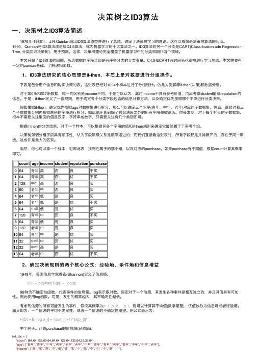
下表是包含⽤户信息和购买决策的表。

这张表已经对1024个样本进⾏了分组统计。

依此为例解释if-then(决策)和数据分组。

对于第0条和第7条数据，唯⼀的区别是income不同，于是可以认为，此时income不具有参考价值，⽽应考察student值或reputation的信息。

于是：if-then定义了⼀套规则，⽤于确定各个分类字段包含的信息计算⽅法，以及确定优先按照哪个字段进⾏分类决策。

假如根据if-then，确定优先按照age对数据集进⾏拆分，那么可以确定三个⽔平(青年、中年、⽼年)对应的⼦数据集。

然后，继续对着三个⼦数据集分别再按照剩余的字段进⾏拆分。

如此循环直到除了购买决策之外的所有字段都被遍历。

你会发现，对于每个拆分的⼦数据集，根本不需要关注⾥⾯的值是汉字、字符串或数字，只需要关注有⼏个类别即可。

根据if-then的分类结果，对于⼀个样本，可以根据其各个字段的值和if-then规则来确定它最终属于下表哪个组。

决策树强调分组字段具有顺序性，认为字段层级关系是层层递进的；⽽我们直接看这张表时，所有字段都是并排展开的，存在于同⼀层级。

id3决策树算法python程序

id3决策树算法python程序关于ID3决策树算法的Python程序。

第一步：了解ID3决策树算法ID3决策树算法是一种常用的机器学习算法，用于解决分类问题。

它基于信息论的概念，通过选择最佳的特征来构建决策树模型。

ID3算法的核心是计算信息增益，即通过选择最能区分不同类别的特征来构建决策树。

第二步：导入需要的Python库和数据集在编写ID3决策树算法的Python程序之前，我们需要导入一些必要的Python库和准备好相关的数据集。

在本例中，我们将使用pandas库来处理数据集，并使用sklearn库的train_test_split函数来将数据集拆分为训练集和测试集。

pythonimport pandas as pdfrom sklearn.model_selection import train_test_split# 读取数据集data = pd.read_csv('dataset.csv')# 将数据集拆分为特征和标签X = data.drop('Class', axis=1)y = data['Class']# 将数据集拆分为训练集和测试集X_train, X_test, y_train, y_test = train_test_split(X, y, test_size=0.2) 第三步：实现ID3决策树算法的Python函数在此步骤中，我们将编写一个名为ID3DecisionTree的Python函数来实现ID3决策树算法。

该函数将递归地构建决策树，直到满足停止条件。

在每个递归步骤中，它将计算信息增益，并选择最佳特征作为当前节点的分裂依据。

pythonfrom math import log2from collections import Counterclass ID3DecisionTree:def __init__(self):self.tree = {}def calc_entropy(self, labels):label_counts = Counter(labels)entropy = 0for count in label_counts.values():p = count / len(labels)entropy -= p * log2(p)return entropydef calc_info_gain(self, data, labels, feature):feature_values = data[feature].unique()feature_entropy = 0for value in feature_values:subset_labels = labels[data[feature] == value]feature_entropy += len(subset_labels) / len(labels) * self.calc_entropy(subset_labels)return self.calc_entropy(labels) - feature_entropydef choose_best_feature(self, data, labels):best_info_gain = 0best_feature = Nonefor feature in data.columns:info_gain = self.calc_info_gain(data, labels, feature)if info_gain > best_info_gain:best_info_gain = info_gainbest_feature = featurereturn best_featuredef build_tree(self, data, labels):if len(set(labels)) == 1:return labels[0]elif len(data.columns) == 0:return Counter(labels).most_common(1)[0][0] else:best_feature = self.choose_best_feature(data, labels)sub_data = {}for value in data[best_feature].unique():subset = data[data[best_feature] == value].drop(best_feature, axis=1)sub_labels = labels[data[best_feature] == value]sub_data[value] = (subset, sub_labels)tree = {best_feature: {}}for value, (subset, sub_labels) in sub_data.items():tree[best_feature][value] = self.build_tree(subset, sub_labels)return treedef fit(self, data, labels):self.tree = self.build_tree(data, labels)def predict(self, data):predictions = []for _, row in data.iterrows():node = self.treewhile isinstance(node, dict):feature = list(node.keys())[0]value = row[feature]node = node[feature][value]predictions.append(node)return predictions第四步：使用ID3决策树模型进行训练和预测最后一步是使用我们实现的ID3DecisionTree类进行训练和预测。

id3算法代码

id3算法代码ID3算法简介ID3算法是一种常用的决策树算法，它通过对数据集的属性进行分析，选择最优属性作为节点，生成决策树模型。

ID3算法是基于信息熵的思想，通过计算每个属性对样本集合的信息增益来选择最优划分属性。

ID3算法步骤1. 计算数据集的熵首先需要计算数据集的熵，熵越大表示样本集合越混乱。

假设有n个类别，则数据集D的熵可以表示为：$$ Ent(D) = -\sum_{i=1}^{n}p_i\log_2p_i $$其中$p_i$表示第i个类别在数据集D中出现的概率。

2. 计算每个属性对样本集合的信息增益接下来需要计算每个属性对样本集合的信息增益。

假设有m个属性，则第j个属性$A_j$对数据集D的信息增益可以表示为：$$ Gain(D, A_j) = Ent(D) - \sum_{i=1}^{v}\frac{|D_i|}{|D|}Ent(D_i) $$其中$v$表示第j个属性可能取值的数量，$D_i$表示在第j个属性上取值为$i$时所包含的样本子集。

3. 选择最优划分属性从所有可用属性中选择最优划分属性作为当前节点。

选择最优划分属性的方法是计算所有属性的信息增益，选择信息增益最大的属性作为当前节点。

4. 递归生成决策树使用选择的最优划分属性将数据集划分成若干子集，对每个子集递归生成子树。

ID3算法代码实现下面是Python语言实现ID3算法的代码：```pythonimport mathimport pandas as pd# 计算熵def calc_entropy(data):n = len(data)label_counts = {}for row in data:label = row[-1]if label not in label_counts:label_counts[label] = 0label_counts[label] += 1entropy = 0.0for key in label_counts:prob = float(label_counts[key]) / n entropy -= prob * math.log(prob, 2) return entropy# 划分数据集def split_data(data, axis, value):sub_data = []for row in data:if row[axis] == value:sub_row = row[:axis]sub_row.extend(row[axis+1:])sub_data.append(sub_row)return sub_data# 计算信息增益def calc_info_gain(data, base_entropy, axis):values = set([row[axis] for row in data])new_entropy = 0.0for value in values:sub_data = split_data(data, axis, value)prob = len(sub_data) / float(len(data))new_entropy += prob * calc_entropy(sub_data) info_gain = base_entropy - new_entropyreturn info_gain# 选择最优划分属性def choose_best_feature(data):num_features = len(data[0]) - 1base_entropy = calc_entropy(data)best_info_gain = 0.0best_feature = -1for i in range(num_features):info_gain = calc_info_gain(data, base_entropy, i)if info_gain > best_info_gain:best_info_gain = info_gainbest_feature = ireturn best_feature# 多数表决函数，用于确定叶子节点的类别def majority_vote(class_list):class_count = {}for vote in class_list:if vote not in class_count:class_count[vote] = 0class_count[vote] += 1sorted_class_count = sorted(class_count.items(), key=lambda x:x[1], reverse=True)return sorted_class_count[0][0]# 创建决策树def create_tree(data, labels):class_list = [row[-1] for row in data]if class_list.count(class_list[0]) == len(class_list):return class_list[0]if len(data[0]) == 1:return majority_vote(class_list)best_feature_idx = choose_best_feature(data)best_feature_label = labels[best_feature_idx]tree_node = {best_feature_label: {}}del(labels[best_feature_idx])feature_values = [row[best_feature_idx] for row in data] unique_values = set(feature_values)for value in unique_values:sub_labels = labels[:]sub_data = split_data(data, best_feature_idx, value) tree_node[best_feature_label][value] =create_tree(sub_data, sub_labels)return tree_node# 预测函数def predict(tree, labels, data):first_str = list(tree.keys())[0]second_dict = tree[first_str]feat_index = labels.index(first_str)key = data[feat_index]value_of_feat = second_dict[key]if isinstance(value_of_feat, dict):class_label = predict(value_of_feat, labels, data) else:class_label = value_of_featreturn class_label# 测试函数def test():# 读取数据集df = pd.read_csv('iris.csv')data = df.values.tolist()# 划分训练集和测试集train_data = []test_data = []for i in range(len(data)):if i % 5 == 0:test_data.append(data[i])else:train_data.append(data[i])# 创建决策树labels = df.columns.tolist()[:-1]tree = create_tree(train_data, labels)# 测试决策树模型的准确率correct_count = 0for row in test_data:true_label = row[-1]pred_label = predict(tree, labels, row[:-1])if true_label == pred_label:correct_count += 1accuracy = float(correct_count) / len(test_data)if __name__ == '__main__':test()```代码解释以上代码实现了ID3算法的主要功能。

matlab实现的ID3 分类决策树算法

function D = ID3(train_features, train_targets, params, region)% Classify using Quinlan's ID3 algorithm% Inputs:% features - Train features% targets - Train targets% params - [Number of bins for the data, Percentage of incorrectly assigned samples at a node]% region - Decision region vector: [-x x -y y number_of_points]%% Outputs% D - Decision sufrace[Ni, M] =size(train_features); %·µ»ØÐÐÊýNiºÍÁÐÊýM%Get parameters[Nbins, inc_node] = process_params(params);inc_node = inc_node*M/100;%For the decision regionN = region(5);mx = ones(N,1) * linspace(region(1),region(2),N); %linspace(ÆðÊ¼Öµ£¬ÖÕÖ¹Öµ£¬ÔªËØ¸öÊý)my = linspace (region(3),region(4),N)' * ones(1,N);flatxy = [mx(:), my(:)]';%Preprocessing[f, t, UW, m] = PCA(train_features,train_targets, Ni, region);train_features = UW * (train_features -m*ones(1,M));flatxy = UW * (flatxy - m*ones(1,N^2));%First, bin the data and the decision region data [H, binned_features]=high_histogram(train_features, Nbins, region); [H, binned_xy] = high_histogram(flatxy, Nbins, region);%Build the tree recursivelydisp('Building tree')tree = make_tree(binned_features,train_targets, inc_node, Nbins);%Make the decision region according to the tree disp('Building decision surface using the tree') targets = use_tree(binned_xy, 1:N^2, tree, Nbins, unique(train_targets));D = reshape(targets,N,N);%ENDfunction targets = use_tree(features, indices, tree, Nbins, Uc)%Classify recursively using a treetargets = zeros(1,size(features,2)); %size(features,2)·µ»Øfeatu resµÄÁÐÊýif (size(features,1) == 1),%Only one dimension left, so work on itfor i = 1:Nbins,in = indices(find(features(indices) == i));if ~isempty(in),if isfinite(tree.child(i)),targets(in) = tree.child(i);else%No data was found in the training set for this bin, so choose it randomallyn = 1 +floor(rand(1)*length(Uc));targets(in) = Uc(n);endendendbreakend%This is not the last level of the tree, so:%First, find the dimension we are to work ondim = tree.split_dim;dims= find(~ismember(1:size(features,1), dim)); %And classify according to itfor i = 1:Nbins,in = indices(find(features(dim, indices) == i));targets = targets + use_tree(features(dims, :), in, tree.child(i), Nbins, Uc);end%END use_treefunction tree = make_tree(features, targets,inc_node, Nbins)%Build a tree recursively[Ni, L] = size(features);Uc = unique(targets);%When to stop: If the dimension is one or the number of examples is smallif ((Ni == 1) | (inc_node > L)),%Compute the children non-recursivelyfor i = 1:Nbins,tree.split_dim = 0;indices = find(features == i);if ~isempty(indices),if(length(unique(targets(indices))) == 1),tree.child(i) =targets(indices(1));elseH =hist(targets(indices), Uc);[m, T] = max(H);tree.child(i) = Uc(T);endelsetree.child(i) = inf;endendbreakend%Compute the node's Ifor i = 1:Ni,Pnode(i) = length(find(targets == Uc(i))) / L; endInode = -sum(Pnode.*log(Pnode)/log(2));%For each dimension, compute the gain ratio impurity delta_Ib = zeros(1, Ni);P = zeros(length(Uc), Nbins);for i = 1:Ni,for j = 1:length(Uc),for k = 1:Nbins,indices = find((targets == Uc(j)) & (features(i,:) == k));P(j,k) = length(indices);endendPk = sum(P);P = P/L;Pk = Pk/sum(Pk);info = sum(-P.*log(eps+P)/log(2));delta_Ib(i) =(Inode-sum(Pk.*info))/-sum(Pk.*log(eps+Pk)/log( 2));end%Find the dimension minimizing delta_Ib[m, dim] = max(delta_Ib);%Split along the 'dim' dimensiontree.split_dim = dim;dims = find(~ismember(1:Ni, dim));for i = 1:Nbins,indices = find(features(dim, :) == i); tree.child(i) = make_tree(features(dims, indices), targets(indices), inc_node, Nbins); end。

【机器学习笔记】ID3构建决策树

【机器学习笔记】ID3构建决策树好多算法之类的，看理论描述，让⼈似懂⾮懂，代码⾛⼀⾛，现象就了然了。

引：from sklearn import treenames = ['size', 'scale', 'fruit', 'butt']labels = [1,1,1,1,1,0,0,0]p1 = [2,1,0,1]p2 = [1,1,0,1]p3 = [1,1,0,0]p4 = [1,1,0,0]n1 = [0,0,0,0]n2 = [1,0,0,0]n3 = [0,0,1,0]n4 = [1,1,0,0]data = [p1, p2, p3, p4, n1, n2, n3, n4]def pred(test):dtre = tree.DecisionTreeClassifier()dtre = dtre.fit(data, labels)print(dtre.predict([test]))with open('treeDemo.dot', 'w') as f:f = tree.export_graphviz(dtre, out_file = f, feature_names = names)pred([1,1,0,1]) 画出的树如下：关于这个树是怎么来的，如果很粗暴地看列的数据浮动情况：或者说是⽅差，⽅差最⼩该是第三列，fruit，然后是butt，scale（⽅差3.0），size（⽅差3.2857）。

再⼀看树节点的分叉情况，fruit，butt，size，scale，两相⽐较，好像发现了什么？衡量数据⽆序度：划分数据集的⼤原则是：将⽆序的数据变得更加有序。

那么如何评价数据有序程度？⽐较直观地，可以直接看数据间的差距，差距越⼤，⽆序度越⾼。

但这显然还不够聪明。

组织⽆序数据的⼀种⽅法是使⽤信息论度量信息。

机器学习-ID3决策树算法（附matlaboctave代码）

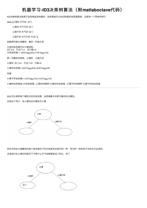
机器学习-ID3决策树算法（附matlaboctave代码）ID3决策树算法是基于信息增益来构建的，信息增益可以由训练集的信息熵算得，这⾥举⼀个简单的例⼦data=[⼼情好天⽓好出门⼼情好天⽓不好出门⼼情不好天⽓好出门⼼情不好天⽓不好不出门]前⾯两列是分类属性，最后⼀列是分类分类的信息熵可以计算得到：出门=3，不出门=1，总⾏数=4分类信息熵 = -(3/4)*log2(3/4)-(1/4)*log2(1/4)第⼀列属性有两类，⼼情好，⼼情不好⼼情好 ,出门=2，不出门=0，⾏数=2⼼情好信息熵=-(2/2)*log2(2/2)+(0/2)*log2(0/2)同理⼼情不好信息熵=-(1/2)*log2(1/2)-(1/2)*log2(1/2)⼼情的信息增益=分类信息熵 - ⼼情好的概率*⼼情好的信息熵 - ⼼情不好的概率*⼼情不好的信息熵由此可以得到每个属性对应的信息熵，信息熵最⼤的即为最优划分属性。

还是这个例⼦，加⼊最优划分属性为⼼情然后分别在⼼情属性的每个具体情况下的分类是否全部为同⼀种，若为同⼀种则该节点标记为此类别，这⾥我们在⼼情好的情况下不管什么天⽓结果都是出门所以，有了⼼情不好的情况下有不同的分类结果，继续计算在⼼情不好的情况下，其它属性的信息增益，把信息增益最⼤的属性作为这个分⽀节点，这个我们只有天⽓这个属性，那么这个节点就是天⽓了，天⽓属性有两种情况，如下图在⼼情不好并且天⽓好的情况下，若分类全为同⼀种，则改节点标记为此类别有训练集可以，⼼情不好并且天⽓好为出门，⼼情不好并且天⽓不好为不出门，结果⼊下图对于分⽀节点下的属性很有可能没有数据，⽐如，我们假设训练集变成data=[⼼情好晴天出门⼼情好阴天出门⼼情好⾬天出门⼼情好雾天出门⼼情不好晴天出门⼼情不好⾬天不出门⼼情不好阴天不出门]如下图：在⼼情不好的情况下，天⽓中并没有雾天，我们如何判断雾天到底是否出门呢？我们可以采⽤该样本最多的分类作为该分类，这⾥天⽓不好的情况下，我们出门=1，不出门=2，那么这⾥将不出门，作为雾天的分类结果在此我们所有属性都划分了，结束递归，我们得到了⼀颗⾮常简单的决策树。

机器学习决策树算法ID3

机器学习决策树算法ID3决策树是一种重要的机器学习算法，它能够处理分类和回归的问题，并且易于理解和解释。

其中，ID3（Iterative Dichotomiser 3）算法是决策树学习中最简单和最流行的一种算法，本文将介绍ID3算法的基本原理和实现过程。

什么是决策树决策树是一种树形结构，其中每个内部节点表示一个属性上的判断，每个叶子节点表示一种分类结果。

决策树的生成分为两个步骤：构建和剪枝。

构建过程是将数据集通过分裂形成一颗完整的决策树；剪枝过程是通过去除不必要的分支来提高模型的泛化能力。

ID3算法的基本原理ID3算法是一种贪心算法，也就是说，在每一次分裂时，它都会选择当前最优的特征进行分裂。

其基本思想是：通过计算某个特征的信息增益来确定每个节点的最优分割策略。

信息增益是指在选择某个特征进行分割后，熵的减少量。

熵的计算公式如下：$$ H(D) = -\\sum_{k=1}^{|y|}p_klog_2p_k $$其中，|y|表示类别的数量，p k表示第k个类别在所有样本中出现的概率。

信息增益的计算公式如下：$$ Gain(D,F) = H(D) - \\sum_{v\\in V(F)}\\frac{|D_v|}{|D|}H(D_v) $$其中，F表示属性，V(F)表示属性F的取值集合。

D v表示选择属性F取值为v时的样本集。

在计算信息增益时，需要选择具有最大信息增益的属性作为分裂属性。

ID3算法的实现过程ID3算法的实现过程可以分为以下几个步骤：1.选择分裂属性：选择信息增益最大的属性作为分裂属性；2.构建节点：将节点标记为分裂属性；3.分裂样本：按照分裂属性将样本集分裂为若干子集；4.递归继续分裂：对于每个子集，递归地执行步骤1到步骤3，直到构建完整个决策树。

具体实现时，可以使用递归函数来实现决策树的构建。

代码如下所示：```python def create_tree(dataset, labels):。

广工ID3决策树算法实验报告

三、实验代码及数据记录1.代码#ID3算法实现代码import pandas as pdimport numpy as npimport timeimport treePlotter as treeplotterdef getData():testdata =pd.read_csv('C:/Users/asus/PycharmProjects/ID3/car_evalution-databases.csv',encoding = "utf-8")# 获取测试数据集特征feature = np.array(testdata.keys())feature = np.array(feature[1:feature.size])# 将测试数据转换成数组S = np.array(testdata)S = np.array(S[:, 1:S.shape[1]])return S,feature#统计某一特征的各个取值的概率def Probability(x):value = np.unique(np.array(x)) #统计某列特征取值类型valueCount = np.zeros(value.shape[0]).reshape(1,value.shape[0])for i in range(0, value.shape[0]):q = np.matrix(x[np.where(x[:,0] == value[i])[0]])valueCount[:,i] = q.shape[0]p = valueCount/valueCount.sum()return p#计算Entropy#S为矩阵类型#返回entropydef Entropy(S):P = Probability(S[:,S.shape[1]-1])logP = np.log(P)entropy = -np.dot(P,np.transpose(logP))[0][0]return entropy#计算EntropyA#S为数组类型#返回最小的信息熵的特征的索引值#返回最小的信息熵值def getMinEntropyA(S):entropy = np.zeros(S.shape[1]-1)for i in range(0, S.shape[1]-1):value = np.unique(np.array(S[:,i]))valueEntropy = np.zeros(value.shape[0]).reshape(1,value.shape[0]) for j in range(0,value.shape[0]):q = np.matrix(S[np.where(S[:,i] == value[j])[0]])valueEntropy[:,j] = Entropy(q)proportion = Probability(np.matrix(S[:, i]).transpose())entropy[i] = np.dot(proportion, valueEntropy.transpose())[0][0] minEntropyA = entropy.min()positionMinEntropA = entropy.transpose().argmin()return positionMinEntropA, minEntropyA#计算Gain#S为数组类型#返回最大信息增益的特征的索引值def getMaxGain(S):entropyS = Entropy(np.matrix(S))positionMinEntropyA, entropyA = getMinEntropyA(S)if(entropyS - entropyA > 0):return positionMinEntropyA#ID3算法#返回ID3决策树def id3Tree(S,features):if(Entropy(np.matrix(S)) == 0):return S[0][S.shape[1] - 1]elif features.size == 1:typeValues = np.unique(S[:, S.shape[1]-1])max = 0maxValue = S[0][S.shape[1] - 1]for value in typeValues:Stemp = np.array(S[np.where(S[:, S.shape[1]-1] == value)[0]]) if max < Stemp.shape[0]:max = Stemp.shape[0]maxValue = valuereturn maxValueelse:bestFeatureIndex = getMaxGain(S)bestFeature = features[bestFeatureIndex]bestFeatureValues = np.unique(S[:, bestFeatureIndex])# 划分S，featurefeatures = delArrary(features, bestFeatureIndex)id3tree = {bestFeature:{}}for value in bestFeatureValues:Stemp = np.array(S[np.where(S[:, bestFeatureIndex] == value)[0]]) Stemp = delArrary(Stemp, bestFeatureIndex)id3tree[bestFeature][value] = id3Tree(Stemp,features)return id3tree#删除数组中的某一列,维数小于2def delArrary(arrary,index):if(arrary.shape[0] == arrary.size):x = np.array(arrary[0:index])y = np.array(arrary[index+1:arrary.shape[0]])return np.array(np.append(x,y))else:x = np.array(arrary[:,0:index])y = np.array(arrary[:,index+1:arrary.shape[1]])return np.array(np.hstack((x,y)))def Classify(tree, feature, S):firstStr = list(tree.keys())[0]secondDict = tree[firstStr]index = list(feature).index(firstStr)for key in secondDict.keys():if S[index] == key:if type(secondDict[key]) != type(1):classlabel = Classify(secondDict[key],feature,S)else:classlabel = secondDict[key]return classlabeltic = time.process_time()S, feature = getData()S2 = np.array(S[30:S.shape[0]])S1 = np.array(S[0:29])a = np.zeros(S1.shape[0],int)b = np.array(S[0:29:,S.shape[1]-1])#生成决策树tree = id3Tree(S, feature)#print(tree)treeplotter.createPlot(tree)print('决策树生成至C:/Users/asus/PycharmProjects/ID3/决策树.png')#生成ID3决策树代码import matplotlib.pyplot as plt"""绘决策树的函数"""decisionNode = dict(boxstyle="round4", color="yellow",fc="1.0") # 定义分支点的样式leafNode = dict(boxstyle="round4", color="green",fc="1.0") # 定义叶节点的样式arrow_args = dict(arrowstyle="<-") # 定义箭头标识样式# 计算树的叶子节点数量def getNumLeafs(myTree):numLeafs = 0firstStr = list(myTree.keys())[0]secondDict = myTree[firstStr]for key in secondDict.keys():if type(secondDict[key]).__name__ == 'dict':numLeafs += getNumLeafs(secondDict[key])else:numLeafs += 1return numLeafs# 计算树的最大深度def getTreeDepth(myTree):maxDepth = 0firstStr = list(myTree.keys())[0]secondDict = myTree[firstStr]for key in secondDict.keys():if type(secondDict[key]).__name__ == 'dict':thisDepth = 1 + getTreeDepth(secondDict[key])else:thisDepth = 1if thisDepth > maxDepth:maxDepth = thisDepthreturn maxDepth# 画出节点def plotNode(nodeTxt, centerPt, parentPt, nodeType):createPlot.ax1.annotate(nodeTxt, xy=parentPt, xycoords='axes fraction', \xytext=centerPt, textcoords='axes fraction', va="center", ha="center",\bbox=nodeType, arrowprops=arrow_args)# 标箭头上的文字def plotMidText(cntrPt, parentPt, txtString):lens = len(txtString)xMid = (parentPt[0] + cntrPt[0]) / 2.0yMid = (parentPt[1] + cntrPt[1]) / 2.0createPlot.ax1.text(xMid, yMid, txtString)def plotTree(myTree, parentPt, nodeTxt):numLeafs = getNumLeafs(myTree)depth = getTreeDepth(myTree)firstStr = list(myTree.keys())[0]cntrPt = (plotTree.x0ff + \(1.0 + float(numLeafs)) / 2.0 / plotTree.totalW, plotTree.y0ff) plotMidText(cntrPt, parentPt, nodeTxt)plotNode(firstStr, cntrPt, parentPt, decisionNode)secondDict = myTree[firstStr]plotTree.y0ff = plotTree.y0ff - 1.0 / plotTree.totalDfor key in secondDict.keys():if type(secondDict[key]).__name__ == 'dict':plotTree(secondDict[key], cntrPt, str(key))else:plotTree.x0ff = plotTree.x0ff + 1.0 / plotTree.totalWplotNode(secondDict[key], \(plotTree.x0ff, plotTree.y0ff), cntrPt, leafNode)plotMidText((plotTree.x0ff, plotTree.y0ff) \, cntrPt, str(key))plotTree.y0ff = plotTree.y0ff + 1.0 / plotTree.totalDdef createPlot(inTree):fig = plt.figure(figsize=(300,15))fig.clf()axprops = dict(xticks=[], yticks=[])createPlot.ax1 = plt.subplot(111, frameon=False, **axprops)plotTree.totalW = float(getNumLeafs(inTree))plotTree.totalD = float(getTreeDepth(inTree))plotTree.x0ff = -0.5 / plotTree.totalWplotTree.y0ff = 1.0plotTree(inTree, (0.5, 1.0), '')plt.savefig(""C:/Users/asus/PycharmProjects/ID3/决策树.png") #plt.show()2.结果截图决策树截图：。

1、下载文档前请自行甄别文档内容的完整性，平台不提供额外的编辑、内容补充、找答案等附加服务。
2、"仅部分预览"的文档,不可在线预览部分如存在完整性等问题,可反馈申请退款(可完整预览的文档不适用该条件!)。
3、如文档侵犯您的权益，请联系客服反馈,我们会尽快为您处理(人工客服工作时间：9:00-18:30)。

机器学习决策树ID3算法的源代码上（VC6.0测试通过）发布: 2009-4-16 11:42 | 作者: 天涯| 来源: 资讯[i=s] 本帖最后由天涯于2009-4-17 13:03 编辑这个的重要，不用多说了吧，有什么意见和建议跟帖留言啊，哈，觉得好，请顶一个第一部分：#include<iostream.h>#include<fstream.h>#include<string.h>#include<stdlib.h>#include<math.h>#include<iomanip.h>#define N 500 //N定义为给定训练数据的估计个数#define M 6 //M定义为候选属性的个数#define c 2 //定义c=2个不同类#define s_max 5 //定义s_max为每个候选属性所划分的含有最大的子集数int av[M]={3,3,2,3,4,2};int s[N][M+2],a[N][M+2]; //数组s[j]用来记录第i个训练样本的第j个属性值int path_a[N][M+1],path_b[N][M+1]; //用path_a[N][M+1],path_b[N][M+1]记录每一片叶子的路径int count_list=M; //count_list用于记录候选属性个数int count=-1; //用count+1记录训练样本数int attribute_test_list1[M];int leaves=1;//用数组ss[k][j]表示第k个候选属性划分的子集Sj中类Ci的样本数，数组的具体大小可根据给定训练数据调整int ss[M][c][s_max];//第k个候选属性划分的子集Sj中样本属于类Ci的概率double p[M][c][s_max];//count_s[j]用来记录第i个候选属性的第j个子集中样本个数int count_s[M][s_max];//分别定义E[M]，Gain[M]表示熵和熵的期望压缩double E[M];double Gain[M];//变量max_Gain用来存储最大的信息增益double max_Gain;int Trip=-1; //用Trip记录每一个叶子递归次数int most;void main(void){int i,j=-1,k,temp,l,count_test,true_class=0,count_train;char trainname[256],testname[256];int test[N][8];cout<<"请输入训练集文件名:";cin>>trainname;ifstream trainfile;trainfile.open(trainname,ios::in|ios::nocreate);if(!trainfile){cout<<"无法使用训练集，请重试!"<<'\n';exit(1);}//读取训练集while(trainfile>>temp){j=j+1;k=j%(M+2);if(k==0||j==0) count+=1;//count为训练集的第几个,k代表室第几个属性switch(k){case 0:s[count][0]=temp;break;case 1:s[count][1]=temp;break;case 2:s[count][2]=temp;break;case 3:s[count][3]=temp;break;case 4:s[count][4]=temp;break;case 5:s[count][5]=temp;break;case 6:s[count][6]=temp;break;case 7:s[count][7]=temp;break;}}trainfile.close();//输出训练集for(i=0;i<=count;i++){if(i%2==0) cout<<'\n';for(j=0;j<M+2;j++)cout<<setw(4)<<s[j];}//most记录训练集中哪类样本数比较多，以用于确定递归终止时不确定的类别for(i=0,j=0,k=0;i<=count;i++){if(s[0]==0) j+=1;else k+=1;}if(j>k) most=0;else most=1;//count_train记录训练集的样本数count_train=count+1;//训练的属性for(i=0;i<M;i++)attribute_test_list1=i+1;//首次调用递归函数，即是生成根结点的分支Generate_decision_tree(s,count+1,attribute_test_list1,count_list,0,0);cout<<'\n'<<"叶子结点的个数为:"<<leaves<<'\n';cout<<"请输入测试集文件名:";cin>>testname;ifstream testfile;testfile.open(testname,ios::in|ios::nocreate);if(!testfile){cout<<"无法使用训练集，请重试!"<<'\n';exit(1);}count_test=0;j=-1;//读取测试集数据while(testfile>>temp){j=j+1;k=j%(M+2);if(k==0) count_test+=1;switch(k){case 0:test[count_test][7]=temp;break;case 1:test[count_test][1]=temp;break;case 2:test[count_test][2]=temp;break;case 3:test[count_test][3]=temp;break;case 4:test[count_test][4]=temp;break;case 5:test[count_test][5]=temp;break;case 6:test[count_test][6]=temp;break;}}testfile.close();for(i=1;i<=count_test;i++)test[0]=0; //以确保评估分类准确率cout<<"count_test="<<count_test<<'\n';cout<<"count_train="<<count_train<<'\n';//用测试集来评估分类准确率for(i=1;i<=count_test;i++){l=0;for(j=1;j<=leaves;j++)if(test[path_b[j][1]]==path_a[j][1]&&test[path_b[j][2]]==path_a[j][2]&&test[path_b[j][3] ]==path_a[j][3]&&test[path_b[j][4]]==path_a[j][4]&&test[path_b[j][5]]==path_a[j][5]&&test[path _b[j][6]]==path_a[j][6]){l=1;if(test[7]==path_a[j][0]) true_class+=1;break;}if(test[7]==most && l==0) true_class+=1;}cout<<"测试集与训练集的比例为:"<<float(count_train)/count_test<<'\n';cout<<"分类准确率为:"<<float(true_class)/count_test<<'\n';}天涯(2009-4-16 11:43:00)第二部分：void Generate_decision_tree(int b[][M+2],int bn,int attribute_test_list[],int sn,int ai,int aj) {//定义数组a记录目前待分的训练样本集，定义数组b记录目前要分结点中所含的训练样本集//same_class用来记数，判别samples是否都属于同一个类Trip+=1;//用Trip记录每一个叶子递归次数path_a[leaves][Trip]=ai;//用path_a[N][M+1],path_b[N][M+1]记录每一片叶子的路径path_b[leaves][Trip]=aj;int same_class,i,j,k,l,ll,lll;if(bn==0){//待分结点的样本集为空时，加上一个树叶，标记为训练集中最普通的类//记录路径与前一路径相同的部分for(i=1;i<Trip;i++)if(path_a[leaves][i]==0){path_a[leaves][i]=path_a[leaves-1][i];path_b[leaves][i]=path_b[leaves-1][i];}cout<<'\n'<<"IF ";for(i=1;i<=Trip;i++)if(i==1) cout<<"a["<<path_b[leaves][i]<<"]="<<path_a[leaves][i];else cout<<"^a["<<path_b[leaves][i]<<"]="<<path_a[leaves][i];cout<<" THEN class="<<most;path_a[leaves][0]=most;//修改树的深度if(path_a[leaves][Trip]==av[path_b[leaves][Trip]-1])for(i=Trip;i>1;i--)if(path_a[leaves][i]==av[path_b[leaves][i]-1]) Trip-=1;elsebreak;Trip-=1;leaves+=1;}else{same_class=1;for(i=0;i<bn-1;i++)if(b[i][0]==b[i+1][0])same_class+=1;if(same_class==bn){//待分样本集属于同一类时以该类标记//记录路径与前一路径相同的部分for(i=1;i<Trip;i++)if(path_a[leaves][i]==0){path_a[leaves][i]=path_a[leaves-1][i];path_b[leaves][i]=path_b[leaves-1][i];}cout<<'\n'<<"IF ";for(i=1;i<=Trip;i++)if(i==1)cout<<"a["<<path_b[leaves][i]<<"]="<<path_a[leaves][i];elsecout<<"^a["<<path_b[leaves][i]<<"]="<<path_a[leaves][i]; cout<<" THEN class="<<b[0][0];path_a[leaves][0]=b[0][0];//修改树的深度if(path_a[leaves][Trip]==av[path_b[leaves][Trip]-1])for(i=Trip;i>1;i--)if(path_a[leaves][i]==av[path_b[leaves][i]-1])Trip-=1;elsebreak;Trip-=1;leaves+=1;//未分类的样本集减少for(i=0,l=-1;i<=count;i++){for(j=0,lll=0;j<bn;j++)if(s[i][M+1]==b[j][M+1])lll++;if(lll==0){l+=1;for(ll=0;ll<M+2;ll++)a[l][ll]=s[i][ll];}}for(i=0,k=-1;i<l;i++){k++;for(ll=0;ll<M+2;ll++)s[k][ll]=a[i][ll];}count=count-bn;}else{if(sn==0){//候选属性集为空时，标记为训练集中最普通的类//记录路径与前一路径相同的部分for(i=1;i<Trip;i++)if(path_a[leaves][i]==0){path_a[leaves][i]=path_a[leaves-1][i];path_b[leaves][i]=path_b[leaves-1][i];}cout<<'\n'<<"IF ";for(i=1;i<=Trip;i++)if(i==1) cout<<"a["<<path_b[leaves][i]<<"]="<<path_a[leaves][i];else cout<<"^a["<<path_b[leaves][i]<<"]="<<path_a[leaves][i]; //判断类别for(i=0,ll=0,lll=0;i<bn;i++){if(b[i][0]==0) ll+=1;else lll+=1;}if(ll>lll) {cout<<" THEN class=0";path_a[leaves][0]=0;}else{cout<<" THEN class=1";path_a[leaves][0]=1;}//修改树的深度if(path_a[leaves][Trip]==av[path_b[leaves][Trip]-1])for(i=Trip;i>1;i--)if(path_a[leaves][i]==av[path_b[leaves][i]-1]) Trip-=1;elsebreak;Trip-=1;leaves+=1;//未分类的样本集减少for(i=0,l=-1;i<=count;i++){for(j=0,lll=0;j<bn;j++)if(s[i][M+1]==b[j][M+1]) lll++;if(lll==0){l+=1;for(ll=0;ll<M+2;ll++)a[l][ll]=s[i][ll];}}for(i=0,k=-1;i<l;i++){k++;for(ll=0;ll<M+2;ll++)s[k][ll]=a[i][ll];}count=count-bn;}else//待分结点的样本集不为空时{//定义count_Positive记录属于正例的样本数int count_Positive=0;//p1,p2分别定义为正负例的比例double p1,p2;double Entropy_Es; //Entropy_Es表示熵for(i=0;i<=count;i++)if(s[i][0]==1)count_Positive+=1;p1=double(count_Positive)/(count+1);p2=1-p1;Entropy_Es=-p1*log10(p1)/log10(2)-p2*log10(p2)/log10(2);cout<<p1<<'\t'<<p2<<'\t'<<Entropy_Es<<'\n';天涯(2009-4-16 11:43:32)继续：//初始化for(i=0;i<sn;i++)//当前的属性包含的个数for(j=0;j<c;j++)//类别for(k=0;k<av[i];k++)//以当前属性分成的小类(每个属性包含的种类数)ss[attribute_test_list[i]-1][j][k]=0;//用数组ss[k][i][j]表示第k个候选属性划分的子集Sj中类Ci的样本数，数组的具体大小可根据给定训练数据调整 for(i=0;i<sn;i++)for(j=0;j<av[i];j++)count_s[attribute_test_list[i]-1][j]=0;//初始化某个属性的某个具体值的全部个数for(i=0;i<count+1;i++)for(j=1;j<=sn;j++)if(s[i][0]==0){//找出每个属性具体某个值属于反例的个数ss[attribute_test_list[j-1]-1][0][s[i][j]-1]+=1;count_s[attribute_test_list[j-1]-1][s[i][j]-1]+=1;}else{ss[attribute_test_list[j-1]-1][1][s[i][j]-1]+=1;count_s[attribute_test_list[j-1]-1][s[i][j]-1]+=1;}//计算分别以各个候选属性划分样本后，各个子集Sj中的样本属于类Ci的概率for(i=0;i<sn;i++)for(j=0;j<c;j++)for(k=0;k<av[i];k++)if(count_s[attribute_test_list[i]-1][k]!=0)p[attribute_test_list[i]-1][j][k]=double(ss[attribute_test_list[i]-1][j][k])/count_s[attribute_test_list[i]-1][k];for(i=0;i<sn;i++)E[attribute_test_list[i]-1]=0.0;//计算熵for(i=0;i<sn;i++)for(j=0;j<av[attribute_test_list[i]-1];j++){//if语句处理0*log10(0)=0if(p[attribute_test_list[i]-1][0][j]==0||p[attribute_test_list[i]-1][1][j]==0) {p[attribute_test_list[i]-1][0][j]=1;p[attribute_test_list[i]-1][1][j]=1;}E[attribute_test_list[i]-1]+=(ss[attribute_test_list[i]-1][0][j]+ss[attribute_test_list[i]-1][1][j])*(-(p[ attribute_test_list[i]-1][0][j]*log10(p[attribute_test_list[i]-1][0][j])/log10(2)+p[attribute_test_list[i]-1][1][j]*log10 (p[attribute_test_list[i]-1][1][j])/log10(2)))/(count+1);}//计算熵的信息增益for(i=0;i<sn;i++)Gain[attribute_test_list[i]-1]=Entropy_Es-E[attribute_test_list[i]-1];//找出信息增益的最大值,用j记录哪个候选属性的信息增益最大max_Gain=Gain[0];j=attribute_test_list[0]-1;for(i=0;i<sn;i++)//找出最大的信息增益if(max_Gain<Gain[attribute_test_list[i]-1]) {max_Gain=Gain[attribute_test_list[i]-1];j=attribute_test_list[i]-1;}//利用得到的具有最大信息增益的属性来划分待分的样本集b[bn][8]int temp[s_max];int b1[N][M+2];int temp1=-1;int temp_b[s_max][N][M+2];for(i=1;i<=av[j];i++){temp[i]=-1;for(k=0;k<bn;k++)//样本的个数if(b[k][j+1]==i){temp[i]+=1;for(l=0;l<M+2;l++)temp_b[i][temp[i]][l]=b[k][l];}}//对于每一个分支使用递归函数重复生成树for(i=1;i<=av[j];i++){for(k=0;k<=temp[i];k++)for(l=0;l<M+2;l++)b1[k][l]=temp_b[i][k][l];if(i==1){for(ll=0,l=0;ll<sn;ll++)if(attribute_test_list[ll]-1!=j) attribute_test_list[l++]=attribute_test_list[ll];Generate_decision_tree(b1,k,attribute_test_list,l,i,j+1);sn-=1;}else{Generate_decision_tree(b1,k,attribute_test_list,sn,i,j+1);if(i==av[j]) attribute_test_list[sn]=j+1;}}}}}}。