Chap015The Term Structure of Interest Rates(金融工程-南开大学,王小麓))
货币银行学The Risk and Term Structure of Interest Rates课件讲义

A bond’s term to maturity also affects its interest rate.
The relationship among interest rates on bonds with different terms to maturity is called the term structure of interest rates.
Risk premium
The spread between the interest rates on bonds with default risk and default-free bonds. It indicates how much additional interest people must earn to be willing to hold a risky bond.
Figure 3 Interest Rate on Municipal and in Treasury Bonds
(a) Market for municipal bonds Price of Bonds, P (P increases↑ )
SC
(b) Default-free(U.S. Treasury)bond market
Price of Bonds, P
Interest Rate, I
(P increases↑ )
(i increases↓ )
ST
P2 T
i2T
i2T
P1 C
i1C
Risk
P1 T
i1T
Premium
P2 C
i2C
Liquidity
Another attribute of a bond that influences its interest rate. The more liquid an asset is, the more desirable it is.
金融市场与金融机构英文课件 (5)

© 2012 Pearson Education. All rights reserved.
5-4
Risk Structure of Interest Rates
Result: Baa-Treasury spread increased from 185 bps to 545 bps.
© 2012 Pearson Education. All rights reserved.
5-15
Liquidity Factor
Another attribute of a bond that influences its interest rate is its liquidity; a liquid asset is one that can be quickly and cheaply converted into cash if the need arises. The more liquid an asset is, the more desirable it is (higher demand), holding everything else constant.
© 2012 Pearson Education. All rige of Long Bonds in the U.S.
© 2012 Pearson Education. All rights reserved.
5-6
Risk Structure of Long Bonds in the U.S.
© 2012 Pearson Education. All rights reserved.
投资学 第11版 Ch15 The Term Structure of Interest Rates
The Yield Curve and Future Interest Rates (2 of 5)
• Yield Curve Under Certainty
• Buy and hold vs. rollover:
1 y2 2 1 r1 1 r2
1
y2
1
r1
1
r2
.5
• (r2) is just enough to make rolling over a series of 1-year bonds equal to investing in the 2-year bond
INVESTMENTS | BODIE, KANE, MARCUS
15-7
Bond Pricing: Two Types of Yield Curves
Pure Yield Curve • Uses stripped or zero
coupon Treasuries
• May differ significantly from the on-the-run yield curve
• Equilibrium requires that both strategies provide the same return
INUS
15-9
Two 2-Year Investment Programs
INVESTMENTS | BODIE, KANE, MARCUS
INVESTMENTS | BODIE, KANE, MARCUS
15-11
The Yield Curve and Future Interest Rates (3 of 5)
• Yield Curve Under Certainty
Chapter 12 The Term Structure of Interest Rates
• so if true,
investors hold ST bonds UNLESS LT bonds offer higher yield as incentive higher yield = liquidity premium
IF LT bond yields have a liquidity premium, then usually LT yields > ST yields or yield curve slopes up.
The Pure Expectations Td buyers do not have any preference about maturity i.e. bonds of different maturities are perfect substitutes
• relationship between yield &
maturity is NOT constant • sometimes short-term yields are highest, • most of the time long-term yields are highest
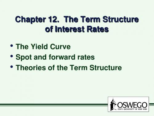
I. The Yield Curve
• assume:
bonds of different maturities are NOT substitutes at all
• if assumption is true,
• separate markets for ST and LT bonds • slope of yield curves tells us nothing about future ST rates unrealistic to assume NO substitution bet. ST and LT bonds
The Term Structure of Interest-Rate Futures Prices, working paper

The Term Structure of Interest-RateFutures Prices.1Richard C.Stapleton2,and Marti G.Subrahmanyam3First draft:June,1994This draft:August13,20011Earlier versions of this paper have been presented at the Workshop on Finan-cial Engineering and Risk Management,European Institute for Advanced Studies in Management,Brussels,and the Chicago Board of Trade Annual European Fu-tures Conference,Rome,and in seminars at New York University,The Federal Reserve Bank of New York,University of Cardiff,University of London,Birkbeck College,The Australian Graduate School of Management,Sydney,The Fields In-stitute,Toronto,and University of California at Los Angeles.We would like to thank T.S.Ho,C.Thanassoulas,S-L.Chung,Q.Dai and O.Grischchenko for helpful comments.We would also like to thank the editor,B.Dumas,and an anonymous referee,whose detailed comments lead to considerable improvements in the paper.We acknowledge able research assistance by V.Acharya,A.Gupta and P.Pasquariello.2Department of Accounting and Finance,University of Strathclyde,100, Cathedral Street,Glasgow,Scotland.Tel:(44)524—381172,Fax:(44)524—846874, Email:rcs@ and University of Melbourne,Australia 3Leonard N.Stern School of Business,New York University,Management Ed-ucation Center,44West4th Street,Suite9—190,New York,NY10012—1126,USA. Tel:(212)998—0348,Fax:(212)995—4233,Email:msubrahm@AbstractThe Term Structure of Interest-Rate FuturesPricesWe derive general properties of two-factor models of the term structure of in-terest rates and,in particular,the process for futures prices and rates.Then, as a special case,we derive a no-arbitrage model of the term structure in which any two futures rates act as factors.In this model,the term structure shifts and tilts as the factor rates vary.The cross-sectional properties of the model derive from the solution of a two-dimensional,autoregressive process for the short-term rate,which exhibits both mean-reversion and a lagged persistence parameter.We show that the correlation of the futures rates is restricted by the no-arbitrage conditions of the model.In addition,we inves-tigate the determinants of the volatilities and the correlations of the futures rates of various maturities.These are shown to be related to the volatility of the short rate,the volatility of the second factor,the degree of mean-reversion and the persistence of the second factor shock.We also discuss the extension of our model to three or more factors.We obtain specific re-sults for futures rates in the case where the logarithm of the short-term rate [e.g.,the London Inter-Bank Offer Rate(LIBOR)]follows a two-dimensional process.We calibrate the model using data from Eurocurrency interest rate futures contracts.Interest Rate Futures1 1IntroductionTheoretical models of the term structure of interest rates are of interest to both practitioners andfinancial academics.The term structure exhibits several patterns of changes over time.In some periods,it shifts up or down, partly in response to higher expectations of future inflation.In other periods, it tilts,with short-term interest rates rising and long-term interest rates falling,perhaps in response to a tightening of monetary policy.Sometimes, its shape changes to an appreciable extent,affecting its curvature.Hence, a desirable feature of a term-structure model is that it should be able to capture shifts,tilts and changes in the curvature of the term structure.In this paper,we present and analyse a model of the term structure of futures rates that has the above properties.Previous work on the term structure of interest rates has concentrated mainly on bond yields of varying maturities or,more recently,on forward rates.In contrast,this paper concentrates on futures rates,partly motivated by the relative lack of previous theoretical models of interest-rate futures prices.However,the main reason for focussing on futures rates is analytical tractability.Futures prices are simple expectations of spot prices under the equivalent martingale measure(EMM),of the future relevant short-term bond prices,whereas forward prices and spot rates involve more complex relationships.It follows that futures prices and futures rates are fairly sim-ple to derive from the dynamics of the spot rate.In contrast,closed-form solutions for forward rates have been obtained only under rather restrictive (e.g.Gaussian)assumptions.Further,from an empirical perspective,since forward and futures rates differ only by a convexity adjustment,it is likely that most of the time series and cross-sectional properties of futures rates are shared by forward rates,to a close approximation,at least for short ma-turity contracts.It makes sense,therefore,to analyse these properties,even if the ultimate goal is knowledge of the term-structure behaviour of forward or spot prices.Finally,the analysis of futures rates is attractive because of the availability of data from trading on organized futures exchanges.Hence, the models derived in the paper are directly testable,using data from the liquid market for Eurocurrency interest rate futures contracts.One contrast between many of the term-structure models presented in the academic literature and those used by practioners for the pricing of interest rate options is in the distributional assumptions made.Most of the modelsInterest Rate Futures2 which derive the term structure,for example Vasicek(1977),Balduzzi,Das, Foresi and Sundaram(1996)(BDFS),Jegadeesh and Pennacchi(1996)(JP), and Gong and Remolona(1997)assume that the short term interest rate is Gaussian.In contrast,popular models for the pricing of interest-rate options often assume that rates are lognormally distributed(see for example Black and Karasinski(1991),Brace,Gatarek and Musiela(1997),and Miltersen, Sandmann and Sondermann(1997)).In this paper,we present a model where the short-term rate LIBOR is assumed to follows a multi-dimensional lognormal process under the EMM.We show that the no-arbitrage futures rates for all maturities are also log-linear in any two(or three)rates.This implies that all futures rates are also lognormal in our model.We then show that the correlation between the long and short maturity futures rates is restricted by the degree of mean-reversion of the short rate and the relative volatilities of the long and short-maturity futures rates.Also,the volatility structure of futures rates of various maturities can be derived explicitly from the assumed process for the spot short rate.The performance of a set of models where the short rate follows a process with a stochastic central tendency has been analysed in a recent article by Dai and Singleton(2000)(DS).They analyse the set of”affine”term struc-ture models introduced previously by Duffie and Kan(1994).Our process for the short rate is also a stochastic central tendency model.However, there are some differences that should be noted between our model and those analysed by DS.First,in our model the short rate follows a discrete-time,rather than a continuous-time process.Second,as noted above,we assume that the process is log-Gaussian.Third,we assume that the short rate follows the process under the risk-neutral measure;hence,we abstract from considerations of the market price of risk.We suggest a time series model in which the short rate follows a stochasic central tendency process.This assumption allows us to nest the AR(1) single-factor model as a special case.It is also general enough to produce stochastic no-arbitrage term structures with shapes that capture most of those observed empirically.A similar model,in which the conditional mean of the short rate is stochastic has been suggested by Hull and White(1994), JP(1996),BDFS(1996)and analysed by Gong and Remolona(1997).The characteristics of these models are reviewed below.The literature on the pricing of futures contracts was pioneered by Cox, Ingersoll and Ross(1981)[CIR],who characterized the futures price of anInterest Rate Futures3 asset as the expectation,under the risk-neutral measure,of the spot price of the asset on the expiration date.In a related paper,Sundaresan(1991) shows that,under the risk-neutral measure,the futures interest rate is the expectation of the spot interest rate in the future.This follows from the fact that the LIBOR futures contract is written on the three-month LIBOR itself,rather than on the price of a zero-coupon instrument.Jegadeesh and Pennacchi(1996)[JP]suggest a two-factor equilibrium model of bond prices and LIBOR futures based on a two-factor extension of the Vasicek(1977)Gaussian model.They assume that the(continuously com-pounded)interest rate is normally distributed and generated by a process with a stochastic central tendency.They then estimate the model using fu-tures prices of LIBOR contracts,backing out estimates of the coefficients of mean-reversion of the short rate as well as the second stochastic conditional-mean factor.Our approach is somewhat different.We directly assume a process for LIBOR,rather than the continuously compounded rate,and then derive the process for the LIBOR futures.1This allows us to analyse the less tractable log-Gaussian case.Our general model is closely related to the JP paper,with the important distinction that it is embedded in an arbitrage-free,rather than an equilib-rium framework,thus eliminating the need for explicitly incorporating the market price of risk.Although our analysis is based on weaker assumptions, we are able to derive quite general,distribution-free results for futures rates. We then include,as a significant special case,a model in which the interest rate is lognormal.The work of Gong and Remolona(1997)is similar,in some respects,to that of JP.Like JP,they also employ a two-factor model,in which the second factor is the conditional mean of the short-rate process.However, they focus on the yield of long-dated bonds rather than on the futures rates. In their model,the short-term rate is linear in the two factors.Also,in a manner similar to Vasicek(1977),they assume a market price of risk,solve for bond prices,and back-out the long-term rates and the variances of the two factors.21This is similar to the approach taken in the LIBOR market models of Brace,Gatarek and Musiela(1997),and Miltersen,Sandmann and Sondermann(1997).2Much of the recent literature,dating back to the work of Ho and Lee(1986),has been concerned with the evolution of forward rates.The most widely cited work in this area is by Heath,Jarrow and Morton[HJM](1990a,1990b,1992).HJM provide a continuous-Interest Rate Futures4 The two-factor models developed in this paper are related also to the expo-nential affine-class of term-structure models introduced by Duffie and Kan (1994).This class is defined as the one where the continuously compounded spot rate is a linear function of any n factors or spot rates.In an interesting special case of our model,where the logarithm of the LIBOR evolves as a two-dimensional linear process,it is the logarithm of the futures rate that is linear in the logarithm of any two futures rates.The remainder of this paper is organised as follows.In section2,we derive some general properties that characterise two-factor models in general and show that if the function of the price of a zero-coupon bond follows a two-dimensional process,its conditional expectation is generated by a two-factor model.We then derive a two-factor,cross-sectional model for futures prices in the general case where a function of the price of a zero-coupon bond follows a stochastic central tendency process.In section3,we assume that the logarithm of the London Inter-Bank Offer Rate(LIBOR)follows a two-dimensional process and derive our main result for futures contracts on the LIBOR:a two-factor cross-sectional relationship between the changes in the prices of interest-rate futures.We estimate the parameters of the two-factor model using estimates of the volatilities and correlations of futures rates derived from the Eurodollar futures contract for the period1995-99, in section4.The conclusions and possible applications of our model to the valuation of interest rate options and to risk management are discussed in section5.Here,we also discuss possible extensions and,in particular,the generalisation of the model to three factors.2Some general properties of two-factor models In this section,we establish two statistical results,that hold for any two-factor process of the form that we assume for the short-term rate.These time limit to the Ho-Lee model and generalize their results to a forward rate which evolves as a generalized Ito-process with multiple factors.The HJM paper can be distinguished from our paper in terms of the inputs to the two frameworks.The required input to the HJM-type models is the term structure of the volatility of forward rates.In contrast,in our paper,we derive the term structure of volatility of futures rates from a more basic assumption regarding the process for the spot rate.To the extent that the futures and forward volatility structures are related,our analysis in this paper provides a link between the spot-rate models of the Vasicek type and the extended HJM-type forward rate models.Interest Rate Futures5 results are used to establish a general proposition,that holds for the condi-tional expectation of any function of the zero-coupon bond price.The con-ditional expectation is of key significance,since the futures price(or rate)is closely related to the conditional expectation of the future spot interest rate. Later in the section,these results are directly applied to establish futures prices and rates.2.1Definitions and notationWe denote P t as the time-t price of a zero-coupon bond paying$1with certainty at time t+m,where m is measured in years.The short-term interest rate is defined in relation to this m-year bond,where m isfixed. The continuously compounded short-term interest rate for m-year money at time t is denoted as i t,where i t=−ln(P t)/m.The London Interbank Offer Rate LIBOR,again for m-year money is denoted r t,where P t=1/(1+r t m), where m is the proportion of a year.3We are concerned with interest rate contracts for delivery at a future date T.We denote the futures rate as F t,T,the rate contracted at t for delivery at T of an m-period loan.We denote the logarithm of the LIBOR futures rate as f t,T=ln[F t,T].Note that,under this notation,which is broadly consistent with HJM,F t,t=r t and f t,t=ln(r t).2.2General properties of two-factor modelsThe two-factor stochastic central tendency models introduced by JP and BDFS have the general form:dx t=k1(θt−x t)dt+σ1dz1(1)dθt=k2(θ−θt)dt+σ2dz2(2) where dz1dz2=ρ1,2dt,and whereρ1,2is the correlation between the Wiener processes dz1and dz2.The coefficients k1and k2measure the degree of mean reversion of the variables to their respective means,θt andθ.σ1and 3In the LIBOR contract,m has to be adjusted for the day-count convention.Hence, m becomes the actual number of days of the loan contract divided by the day-count basis (usually360or365days).Interest Rate Futures6σ2are the instantaneous standard deviations of the variables x andθ.In JP,x t=i t is the continuously compounded short-term interest rate.The central tendencyθt is interpreted as either a“federal funds target”or as reflecting“investors’rational expectations of longer-term inflation.”In the paper by BDFS,x t is again the short-term interest rate.However,they suggest a slightly more general process for the central tendencydθt=k2(θ−θt+a)dt+σ2dz2(3) The constant allows for a drift in the central tendency.In both models,the short-term interest rate is normally distributed.Essentially,these models are two-factor extensions of the one-factor Vasicek (1977)model.A similar extension is made in Hull and White(1994),with a slightly different assumption that allows the drift of the short-term interest rate to be time dependent.Hull and White assume that x t is any function of the short rate,for example;if x t=ln(i t),where i t is the continuously compounded short term rate,then the model is a two-factor extension of the lognormal Black and Karasinski model.Hull and White state the model in a slightly different form from that of JP and BDFS:dx t=(φt+u t−k1x t)dt+σ1dz1(4)du t=−k2u t dt+σ02dz2(5) However,this model can be shown to be a simple transformation of the BDFS model,with the generalisation that the drift term a is time dependent, i.e.(3)contains a term a t.4In this paper,we consider the general Hull-White class of two-factor models. In discrete form,these models have the following general structure:5.x t+1−x t=c(φt−x t)+y t+²t+1(8) 4Letφt=k1θt−u t,(6)σ02=k1σ2.(7) Then substitution of equations(6)and(7)in equations(4)and(5)yields the general BDFS model(1)and(3).5Dai and Singleton(2000),in the discussion following their equation(20),argue that models of this type,with the additional restriction that the innovations in r t andθt are uncorrelated,fail to capture the empirical term structure of volatility.They suggest thatInterest Rate Futures7y t+1−y t=−αy t+νt+1,(9)E(²t+1)=E(νt+1)=0(10)wherec=1−e−k1nα=1−e−k2n,and n is the length of the time period.In this model,y t has an initial value of zero and mean reverts to zero.6It follows that E(y t)=0,and hence, taking expectations in equation(8),E(x t+1)−E(x t)=c(φt−x t)Then,substituting back in equation(8)we havex t+1−E(x t+1)=(1−c)[x t−E(x t)]+y t+²t+1(11) Hence,in this type of model,the value of x t reverts at the rate c to its initial expected value.We now establish that,if a variable follows the above process,the conditional expectation of the variable is necessarily governed by a two-factor cross-sectional model.We begin by proving this result quite generally,and then apply it to the special case where x t is an interest rate or its logarithm.Lemma1The variable x t follows the processx t+1−E(x t+1)=(1−c)[x t−E(x t)]+y t+²t+1wherey t+1−y t=−αy t+νt+1if and only if the conditional expectation of x t+k is of the formE t(x t+k)=a k x t+b k E t(x t+1)humped shaped volatility term structures are not possible in the above model and the volatility structure is monotonic.However,as shown,for example,by Hull and White (1994),Figure3,this is not true.The simulations in Section4below also illustrate this point in some detail for the case of futures rate volatilities.6See Hull and White(1994),footnote4.Interest Rate Futures8 whereb k=kXτ=1(1−c)k−τ(1−α)τ−1(12)a k=(1−c)k−(1−c)b k.(13)Proof.See appendix1.First,let us take the simplest case where x is the short-term rate of interest. The lemma then implies that if the short rate follows the Hull-White process, the expectation of the short rate k periods hence,is linear in the short rate and the expectation of the short rate at t=1.The implication of this result can be illustrated as follows.Under the expectations hypothesis,where the forward rate is the expectation of the future spot rate,it follows that the k-th period forward rate is a linear function of the spot rate and the t=1 forward rate.One important implication of the lemma is that in this type of two-factor model,the cross-sectional linear coefficients a k and b k are invariant to the in-terchange of the mean reversion coefficient,c and the persistence parameter,α.That isa k,b k|c,α=a k,b k|c0,α0,if c0=α,andα0=c.This identification problem means that it may be difficult to distinguish models where the interest rate reverts very rapidly to a slowly decaying central tendency,from those where the interest rate reverts slowly to a rapidly decaying central tendency.7Lemma1states the implications of a two-dimensional,stochastic conditional mean,process for an arbitrary function of the zero-coupon bond price.The function could be a rate of interest,such as the continuously compounded rate(as in HJM)or the LIBOR(as in BGM),or it could be any other function of the price of the zero-coupon bond itself.The lemma restricts the cross-sectional properties of the conditional expectation.As we will 7This partially explains why,in the calibration of the model in section4,there are two sets of parameters that yield exactly the same volatilities and correlations of the futures rates.It may also explain discrepancies in empirical results presented in JP,DS and others.Interest Rate Futures9 see in the following section,these properties are directly relevant for the investigation of futures prices and rates.The intuition behind Lemma1is that the two influences on the function of the zero-bond prices,one of which is lagged,yield a cross-sectional structure with two factors.2.3Interest-Rate Futures Prices in a No-Arbitrage Economy In this sub-section,we apply the results in the previous sub-section to de-rive futures prices and futures interest rates in a no-arbitrage setting.We assume here that the two-dimensional process,specified in equation(11) for x t=f(P t),holds under the Equivalent Martingale Measure(EMM). The EMM is the measure under which all zero-coupon bond prices,nor-malised by the money market account,follow martingales.Assuming that the process followed by x t is of the Hull-White type under the risk-neutral measure abstracts from considerations of the market price of risk.It allows us to directly derive prices for futures contracts on x t.Cox,Ingersoll and Ross(1981)and Jarrow and Oldfield(1981)established the proposition that the futures price,of any asset,is the expected value of the future spot price of the asset,where the expected value is taken with respect to the equivalent martingale measure.We can now apply this result to determine futures prices,assuming that a function of the bond price is generated by the two-dimensional process analysed above.Since there is a one-to-one relationship between zero-coupon bond prices and short-term interest rates,defined in a particular way,we can then proceed to derive a model for futures interest rates.Initially,we make no specific distributional assumptions.We assume only a)a no-arbitrage economy in which the EMM exists,b)that x t,which is some function of the time t price of an m-year zero-coupon bond,follows a stochasic central tendency process of the general form assumed in Lemma 1,and c)that a market exists for trading futures contracts on x t,where the contracts are marked-to-market at the same frequency as the definition of the discrete time-period from t to t+1.Wefirst establish a general result, and then illustrate it with some familiar examples.We denote the futures price,at t,for delivery of x t+k at t+k,as x t,k.We now have: Proposition1(General Cross-Sectional Relationship for Futures Prices)Interest Rate Futures10 Assume that equation(11)holds for x t under the EMM,where x t=f(P t), then the k-period ahead futures price of x t is given by the two-factor linear relationship:x t,k−x0,k=a k[x t−x0,t]+b k[x t,t+1−x0,t+1]whereb k=kXτ=1(1−c)k−τ(1−α)τ−1(14)a k=(1−c)k−(1−c)b k.(15) Proof.From CIR(1981),proposition2and Pliska(1997),the futures price of any payoffis its expected value,under the EMM.Applying this result to x t+k,yieldsx t,k=E t(x t+k)(16) Substituting equation(16)in Lemma1yields the statement in the Propo-sition.2The rather general result in Proposition1is of principal interest because of two special cases.Thefirst is the case where the futures contract is on the zero-coupon bond itself.The second is the case of a futures contract on an interest rate,such as LIBOR,which is a function of the zero-coupon bond price.Thefirst case is typified by the T.Bill futures contract traded on the Sydney Futures Exchange.The second case is the most common, typified by the Eurocurrency futures contract.We consider these cases in the corollaries below.RemarkAn interesting implication of Proposition1is that if the bond price itself follows a linear process,under the EMM,then the futures prices of the bond will be given by a two-factor cross-sectional relationship.This follows by assuming that x t=f(P t)=P t in the Proposition.This shows that futures prices at time t are generated by a linear two-factor model,if and only if the zero-bond price follows a process of the Hull-White type.Note that the two factors generating the k th futures price are the spot price of the bond and thefirst futures price,i.e.,the futures with maturity equal to t+1.Interest Rate Futures11 Similarly,the variance of the k th futures price is determined by the variance of the spot bond price,the variance of the conditional mean and the mean-reversion coefficients.This is helpful in understanding the conditions under which the term structure follows a two-factor process.Essentially,if futures prices of long-dated futures contracts are given by the cross-sectional model in Proposition1,then forward prices,and also futures and forward rates will follow two-factor models.The relationship for interest rates,however, is,in general,complex,since the functions i t(P t)and r t(P t)are non-linear.We now illustrate the use of Proposition1in the case of interest rate(as opposed to bond-price)futures.Instead of assuming that the price of a zero-coupon bond follows a two-dimensional,linear process,we now assume that the interest rate,LIBOR,follows a stochastic central tendency process. We have the following corollary of Proposition1:Corollary1(Cross-Sectional Relationship for LIBOR Futures Prices for the Case of a Linear Process for the LIBOR)In a no-arbitrage economy,the short-term rate of interest follows a process of the formr t+1=E0[r t+1]+(1−c)[r t−E0(r t)]+y t+²t+1(17) wherey t+1−y t=−αy t+νt+1andE t(²t+1)=0,E t(νt+1)=0,if and only if the term structure of futures rates at time t is generated by a two-factor model,where the k th futures rate is given byr t,k−r0,t+k=a k[r t−r0,t]+b k[r t,t+1−r0,t+1](18) where a k and b k are given by(15)and(14)respectively.Interest Rate Futures12 Proof.The proof of the corollary again follows as a special case of Proposi-tion1,where x t=r t.2The corollary illustrates the simple two-factor structure of futures rates that is implied by the two-dimensional process for the spot rate.Note that the mean-reversion coefficients are embedded in the cross-sectional coefficients, a k and b k.Also,given the linear structure,it follows from(18),that the futures rates will be normally distributed,if the spot rate and thefirst futures rate are normally distributed.Hence,the corollary could be helpful in building a Gaussian model of the term structure of futures rates.83LIBOR futures prices in a lognormal short-rate modelIn the previous section,we showed that if the short-term LIBOR interest rate,evolves as a two-dimensional mean-reverting process under the risk-neutral measure,then a simple cross-sectional relationship exists between futures rates of various maturities.In principle,this type of model could be applied to predict relationships between the prices of Eurocurrency futures contracts,based on LIBOR or some other similar reference rate,which are the most important short-term interest rate futures contracts traded on the markets.However,in the case of LIBOR,the consensus in the academic literature and in market practice is that changes in interest rates are depen-dent on the level of interest rates.In particular,a lognormal distribution for short-term interest rates is commonly assumed.9When the logarithm of the short-term interest rate follows a linear process, the results of the analysis of futures prices in section2cannot be used directly,since the market does not trade futures on the logarithm of the LI-8In a two-factor extension of the Vasicek(1977)framework,JP(1996)estimate a two-factor term structure model that is similar to that in equation(18)under the assumption of normally distributed interest rates.They show that their modelfits the level of Eurodollar short-term interest rates contracts rather well for maturities of up to two years,and changes in the rates for longer-dated contracts.It is possible that this is because of ignoring the skewness effect(due to the normality assumption),which becomes significant for longer-dated contracts.9This is borne out by the empirical research of Chan et.al.,(1992)and more recently of Eom(1994)and Bliss and Smith(1998).There continues to be debate over the elasticity parameter of the changes in interest rates with respect to the level.。
The Term Structure of Interest Rates, Forward Contracts, and Futures

5
The Theory of Term Structure Forward Rates
The unbiased expectations theory attempts to explain observed forward rates by saying that expected future rates will, on average, be equal to the implied forward rates.
a. The liquidity premium added to a decreasing term structure b. The liquidity premium added to a increasing term structure
12
For page 11
For page 12
For page 14
The Term Structure of Interest Rates, Forward Contracts, and Futures
Section 1: The Term Structure of Interest Rates
The Yield to Maturity
2
3
The Theory of Term Structure Forward Rates
15
16
Section 2: Models of the Term Structure
Models of the term structure: Two categories Equilibrium Model: specify a process for the short-term interest rate that is based on assumptions about economic variables, not automatically fit market data on the term structure of interest rate at any point in time Arbitrage-free Model: calibrated to fit market data
投资学investment 题库Chap015
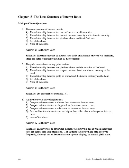
Multiple Choice Questions1. The term structure of interest rates is:A) The relationship between the rates of interest on all securities.B) The relationship between the interest rate on a security and its time to maturity.C) The relationship between the yield on a bond and its default rate.D) All of the above.E) None of the above.Answer: B Difficulty: EasyRationale: The term structure of interest rates is the relationship between two variables, years and yield to maturity (holding all else constant).2. The yield curve shows at any point in time:A) The relationship between the yield on a bond and the duration of the bond.B) The relationship between the coupon rate on a bond and time to maturity of thebond.C) The relationship between yield on a bond and the time to maturity on the bond.D) All of the above.E) None of the above.Answer: C Difficulty: EasyRationale: See rationale for question 15.1.3. An inverted yield curve implies that:A) Long-term interest rates are lower than short-term interest rates.B) Long-term interest rates are higher than short-term interest rates.C) Long-term interest rates are the same as short-term interest rates.D) Intermediate term interest rates are higher than either short- or long-term interestrates.E) none of the above.Answer: A Difficulty: EasyRationale: The inverted, or downward sloping, yield curve is one in which short-term rates are higher than long-term rates. The inverted yield curve has been observedfrequently, although not as frequently as the upward sloping, or normal, yield curve.4. An upward sloping yield curve is a(n) _______ yield curve.A) normal.B) humped.C) inverted.D) flat.E) none of the above.Answer: A Difficulty: EasyRationale: The upward sloping yield curve is referred to as the normal yield curve, probably because, historically, the upward sloping yield curve is the shape that has been observed most frequently.5. According to the expectations hypothesis, a normal yield curve implies thatA) interest rates are expected to remain stable in the future.B) interest rates are expected to decline in the future.C) interest rates are expected to increase in the future.D) interest rates are expected to decline first, then increase.E) interest rates are expected to increase first, then decrease.Answer: C Difficulty: EasyRationale: An upward sloping yield curve is based on the expectation that short-term interest rates will increase.6. Which of the following is not proposed as an explanation for the term structure ofinterest rates:A) The expectations theory.B) The liquidity preference theory.C) The market segmentation theory.D) Modern portfolio theory.E) A, B, and C.Answer: D Difficulty: EasyRationale: A, B, and C are all theories that have been proposed to explain the term structure.7. The expectations theory of the term structure of interest rates states thatA) forward rates are determined by investors' expectations of future interest rates.B) forward rates exceed the expected future interest rates.C) yields on long- and short-maturity bonds are determined by the supply and demandfor the securities.D) all of the above.E) none of the above.Answer: A Difficulty: EasyRationale: The forward rate equals the market consensus expectation of future short interest rates.8. Which of the following theories state that the shape of the yield curve is essentiallydetermined by the supply and demands for long-and short-maturity bonds?A) Liquidity preference theory.B) Expectations theory.C) Market segmentation theory.D) All of the above.E) None of the above.Answer: C Difficulty: EasyRationale: Market segmentation theory states that the markets for different maturities are separate markets, and that interest rates at the different maturities are determined by the intersection of the respective supply and demand curves.9. If forward rates are known with certainty and all bonds are fairly pricedA) all bonds would have the same yield to maturity.B) all short-maturity bonds would have lower prices than all long-maturity bonds.C) all bonds would have the same price.D) all bonds would provide equal 1-year rates of return.E) none of the above.Answer: D Difficulty: EasyRationale: In a world of perfect certainty, all bond must offer equal rates of return over any holding period; otherwise, at least one bond would be dominated by the others in that this bond would offer a lower rate of return than would combinations of other bonds.No one would be willing to hold this bond, and the price of the bond would decline (law of one price).10. According to the "liquidity preference" theory of the term structure of interest rates, theyield curve usually should be:A) inverted.B) normal.C) upward sloping.D) A and B.E) B and C.Answer: E Difficulty: EasyRationale: According to the liquidity preference theory, investors would prefer to beliquid rather than illiquid. In order to accept a more illiquid investment, investorsrequire a liquidity premium and the normal, or upward sloping, yield curve results. Use the following to answer questions 11-14:Suppose that all investors expect that interest rates for the 4 years will be as follows:Year Forward Interest Rate0 (today)5%1 7%2 9%3 10%11. What is the price of 3-year zero coupon bond with a par value of $1,000?A) $863.83B) $816.58C) $772.18D) $765.55E) none of the aboveAnswer: B Difficulty: ModerateRationale: $1,000 / (1.05)(1.07)(1.09) = $816.5812. If you have just purchased a 4-year zero coupon bond, what would be the expected rateof return on your investment in the first year if the implied forward rates stay the same?(Par value of the bond = $1,000)A) 5%B) 7%C) 9%D) 10%E) none of the aboveAnswer: A Difficulty: ModerateRationale: The forward interest rate given for the first year of the investment is given as 5% (see table above).13. What is the price of a 2-year maturity bond with a 10% coupon rate paid annually? (Parvalue = $1,000)A) $1,092.97B) $1,054.24C) $1,000.00D) $1,073.34E) none of the aboveAnswer: D Difficulty: ModerateRationale: [(1.05)(1.07)]1/2 - 1 = 6%; FV = 1000, n = 2, PMT = 100, i = 6, PV =$1,073.3414. What is the yield to maturity of a 3-year zero coupon bond?A) 7.00%B) 9.00%C) 6.99%D) 7.49%E) none of the aboveAnswer: C Difficulty: ModerateRationale: [(1.05)(1.07)(1.09)]1/3 - 1 = 6.99.Use the following to answer questions 15-18:The following is a list of prices for zero coupon bonds with different maturities and par value of $1,000.Maturity (Years) Price1 $943.402 $881.683 $808.884 $742.0915. What is, according to the expectations theory, the expected forward rate in the thirdyear?A) 7.00%B) 7.33%C) 9.00%D) 11.19%E) none of the aboveAnswer: C Difficulty: ModerateRationale: 881.68 / 808.88 - 1 = 9%16. What is the yield to maturity on a 3-year zero coupon bond?A) 6.37%B) 9.00%C) 7.33%D) 10.00%E) none of the aboveAnswer: C Difficulty: ModerateRationale: (1000 / 808.81)1/3 -1 = 7.33%17. What is the price of a 4-year maturity bond with a 12% coupon rate paid annually? (Parvalue = $1,000)A) $742.09B) $1,222.09C) $1,000.00D) $1,141.92E) none of the aboveAnswer: D Difficulty: DifficultRationale: (1000 / 742.09)1/4 -1 = 7.74%; FV = 1000, PMT = 120, n = 4, i = 7.74, PV = $1,141.9218. You have purchased a 4-year maturity bond with a 10% coupon rate paid annually. Thebond has a par value of $1,000. What would the price of the bond be one year from now if the implied forward rates stay the same?A) $808.88B) $1,108.88C) $1,000D) $1,042.78E) none of the aboveAnswer: D Difficulty: DifficultRationale: (943.40 / 742.09)]1/3 - 1.0 = 8.33%; FV = 1000, PMT = 100, n = 3, i = 8.33, PV = $1,042.7819. The market segmentation theory of the term structure of interest ratesA) theoretically can explain all shapes of yield curves.B) definitely holds in the "real world".C) assumes that markets for different maturities are separate markets.D) A and B.E) A and C.Answer: E Difficulty: EasyRationale: Although this theory is quite tidy theoretically, both investors and borrows will depart from their "preferred maturity habitats" if yields on alternative maturities are attractive enough.20. Given the following pattern of forward rates:Year Forward Rate1 5%2 6%3 6.5%If one year from now the term structure of interest rates changes so that it looks exactly the same as it does today, what would be your holding period return if you purchased a 3-year zero coupon bond today and held it for one year?A) 6%B) 8%C) 9%D) 5%E) none of the aboveAnswer: D Difficulty: DifficultRationale: $1,000 / (1.06)(1.065) = $885.82 (selling price); $1,000 / (1.05)(1.06)(1.065) = $843.64 (purchase price); ($885.82 - $843.64) / $843.64 = 5%.21. An upward sloping yield curveA) is an indication that interest rates are expected to increase.B) incorporates a liquidity premium.C) reflects the confounding of the liquidity premium with interest rate expectations.D) all of the above.E) none of the above.Answer: D Difficulty: EasyRationale: One of the problems of the most commonly used explanation of termstructure, the expectations hypothesis, is that it is difficult to separate out the liquidity premium from interest rate expectations.22. The "break-even" interest rate for year n that equates the return on an n-periodzero-coupon bond to that of an n-1-period zero-coupon bond rolled over into a one-year bond in year n is defined asA) the forward rate.B) the short rate.C) the yield to maturity.D) the discount rate.E) None of the above.Answer: A Difficulty: EasyRationale: The forward rate for year n, fn, is the "break-even" interest rate for year n that equates the return on an n-period zero- coupon bond to that of an n-1-periodzero-coupon bond rolled over into a one-year bond in year n.23. When computing yield to maturity, the implicit reinvestment assumption is that theinterest payments are reinvested at the:A) Coupon rate.B) Current yield.C) Yield to maturity at the time of the investment.D) Prevailing yield to maturity at the time interest payments are received.E) The average yield to maturity throughout the investment period.Answer: C Difficulty: ModerateRationale: In order to earn the yield to maturity quoted at the time of the investment, coupons must be reinvested at that rate.24. Which one of the following statements is true?A) The expectations hypothesis indicates a flat yield curve if anticipated futureshort-term rates exceed the current short-term rate.B) The basic conclusion of the expectations hypothesis is that the long-term rate isequal to the anticipated long-term rate.C) The liquidity preference hypothesis indicates that, all other things being equal,longer maturities will have lower yields.D) The segmentation hypothesis contends that borrows and lenders are constrained toparticular segments of the yield curve.E) None of the above.Answer: D Difficulty: ModerateRationale: A flat yield curve indicates expectations of existing rates. Expectationshypothesis states that the forward rate equals the market consensus of expectations of future short interest rates. The reverse of c is true.25. The concepts of spot and forward rates are most closely associated with which one ofthe following explanations of the term structure of interest rates.A) Segmented Market theoryB) Expectations HypothesisC) Preferred Habitat HypothesisD) Liquidity Premium theoryE) None of the aboveAnswer: B Difficulty: ModerateRationale: Only the expectations hypothesis is based on spot and forward rates. A andC assume separate markets for different maturities; liquidity premium assumes higheryields for longer maturities.26.Par Value $1,000Time to Maturity 20 yearsCoupon 10% (paid annually)Current Price $850Yield to Maturity 12%Given the bond described above, if interest were paid semi-annually (rather thanannually), and the bond continued to be priced at $850, the resulting effective annual yield to maturity would be:A) Less than 12%B) More than 12%C) 12%D) Cannot be determinedE) None of the aboveAnswer: B Difficulty: ModerateRationale: FV = 1000, PV = -850, PMT = 50, n = 40, i = 5.9964 (semi-annual);(1.059964)2 - 1 = 12.35%.27. Interest rates might declineA) because real interest rates are expected to decline.B) because the inflation rate is expected to decline.C) because nominal interest rates are expected to increase.D) A and B.E) B and C.Answer: D Difficulty: EasyRationale: The nominal rate is comprised of the real interest rate plus the expected inflation rate.28. Statistical estimation of the yield curve contains apparent pricing error. These errorterms are probably a result ofA) tax effects.B) call provisions.C) out of date price quotes.D) all of the above.E) none of the above.Answer: D Difficulty: EasyRationale: All of the factors listed can cause what appear to be pricing errors but are actually reflective of inaccurate reporting, differences in investor tax status, anddifferences in bond indentures.29. Forward rates ____________ future short rates because ____________.A) are equal to; they are both extracted from yields to maturity.B) are equal to; they are perfect forecasts.C) differ from; they are imperfect forecasts.D) differ from; forward rates are estimated from dealer quotes while future short ratesare extracted from yields to maturity.E) are equal to; although they are estimated from different sources they both are usedby traders to make purchase decisions.Answer: C Difficulty: EasyRationale: Forward rates are the estimates of future short rates extracted from yields to maturity but they are not perfect forecasts because the future cannot be predicted with certainty; therefore they will usually differ.30. The pure yield curve can be estimatedA) by using zero-coupon bonds.B) by using coupon bonds if each coupon is treated as a separate "zero."C) by using corporate bonds with different risk ratings.D) by estimating liquidity premiums for different maturities.E) A and B.Answer: E Difficulty: ModerateRationale: The pure yield curve is calculated using zero coupon bonds, but coupon bonds may be used if each coupon is treated as a separate "zero."31. The market segmentation and preferred habitat theories of term structureA) are identical.B) vary in that market segmentation is rarely accepted today.C) vary in that market segmentation maintains that borrowers and lenders will notdepart from their preferred maturities and preferred habitat maintains that market participants will depart from preferred maturities if yields on other maturities areattractive enough.D) A and B.E) B and C.Answer: E Difficulty: ModerateRationale: Borrowers and lenders will depart from their preferred maturity habitats if yields are attractive enough; thus, the market segmentation hypothesis is no longer readily accepted.32. The yield curveA) is a graphical depiction of term structure of interest rates.B) is usually depicted for U. S. Treasuries in order to hold risk constant acrossmaturities and yields.C) is usually depicted for corporate bonds of different ratings.D) A and B.E) A and C.Answer: D Difficulty: EasyRationale: The yield curve (yields vs. maturities, all else equal) is depicted for U. S.Treasuries more frequently than for corporate bonds, as the risk is constant across maturities for Treasuries.Use the following to answer questions 33-36:Year 1-Year Forward Rate1 5.8%2 6.4%3 7.1%4 7.3%5 7.4%33. What should the purchase price of a 2-year zero coupon bond be if it is purchased at thebeginning of year 2 and has face value of $1,000?A) $877.54B) $888.33C) $883.32D) $893.36E) $871.80Answer: A Difficulty: DifficultRationale: $1,000 / [(1.064)(1.071)] = $877.5434. What would the yield to maturity be on a four-year zero coupon bond purchased today?A) 5.80%B) 7.30%C) 6.65%D) 7.25%E) none of the above.Answer: C Difficulty: ModerateRationale: [(1.058) (1.064) (1.071) (1.073)]1/4 - 1 = 6.65%35. Calculate the price at the beginning of year 1 of a 10% annual coupon bond with facevalue $1,000 and 5 years to maturity.A) $1,105.47B) $1,131.91C) $1,177.89D) $1,150.01E) $719.75Answer: B Difficulty: DifficultRationale: i = [(1.058) (1.064) (1.071) (1.073) (1.074)]1/5 - 1 = 6.8%; FV = 1000, PMT = 100, n = 5, i = 6.8, PV = $1,131.9136. What should be the holding period return of a 9% annual coupon bond with face value$1000 and five years to maturity if it is purchased at the beginning of year 1 and sold at the beginning of year 2, assuming that rates do not change.A) 6.0%B) 7.1%C) 6.8%D) 7.4%E) none of the above.Answer: A Difficulty: DifficultRationale: Using the information in 15.36, P0 = $1,131.91; i = [(1.064) (1.071) (1.073)(1.074)]1/4 - 1 = 7.05%; FV = 1000, PMT = 100, n = 4, i = 7.05, PV = $1,099.81; HPR =(1099.81 - 1131.91 + 100) / 1131.91 = 6%.37. Given the yield on a 3 year zero-coupon bond is 7.2% and forward rates of 6.1% in year1 and 6.9% in year 2, what must be the forward rate in year 3?A) 7.2%B) 8.6%C) 6.1%D) 6.9%E) none of the above.Answer: B Difficulty: ModerateRationale: f3 = (1.072)3 / [(1.061) (1.069)] - 1 = 8.6%38. Consider two annual coupon bonds, each with two years to maturity. Bond A has a 7%coupon and a price of $1000.62. Bond B has a 10% coupon and sells for $1,055.12.Find the two one-period forward rates that must hold for these bonds.A) 6.97%, 6.95%B) 6.95%, 6.95%C) 6.97%, 6.97%D) 6.08%, 7.92%E) 7.00%, 10.00%Answer: D Difficulty: DifficultRationale: 1000.62 = d1 X 70 + d2 X 1070;1055.12 = d1 X 100 + d2 X 1100;2620.36 = 3000 d2;d2 = .8735; d1 = .9427; r1 = 6.08%; r2 = 7.92%.39. An inverted yield curve is oneA) with a hump in the middle.B) constructed by using convertible bonds.C) that is relatively flat.D) that plots the inverse relationship between bond prices and bond yields.E) that slopes downward.Answer: E Difficulty: EasyRationale: An inverted yield curve occurs when short-term rates are higher thanlong-term rates.40. Assuming the forecasts implicit in a yield curve come to pass, an inverted yield curvewould be most favorable forA) short-term borrowers.B) long-term borrowers.C) short-term lenders.D) long-term lenders.E) nobody - Neither a borrower nor a lender be.Answer: D Difficulty: DifficultRationale: Short-term borrowers would face high interest rates. Long-term borrowers would lock in a higher rate than necessary. Short-term lenders would earn a high rate initially, but later would earn lower rates. Long-term lenders would lock in higherinterest rates than they could in the future. Note: If lower rates occur later, some of the long-term borrowers may choose to prepay their loans.41. Investors can use publicly available financial date to determine which of the following?I)the shape of the yield curveII)future short-term ratesIII)the direction the Dow indexes are headingIV)the actions to be taken by the Federal ReserveA) I and IIB) I and IIIC) I, II, and IIID) I, III, and IVE) I, II, III, and IVAnswer: A Difficulty: ModerateRationale: Only the shape of the yield curve and future inferred rates can be determined.The movement of the Dow Indexes and Federal Reserve policy are influenced by term structure but are determined by many other variables also.42. Which of the following is a reason that bond prices do not conform exactly to thepresent value of the bond's cash flows?I) A call feature affects the bond's price.II)After-tax cash flows may be different for different investors.III)The IRS may impute a “built-in” interest payment.IV)Some investors might choose to sell the bond before its maturity date.A) I and IIB) I, II, and IIIC) I and IVD) I, II, and IVE) I, II, III and IVAnswer: E Difficulty: ModerateRationale: All of the items listed can affect the actual cash flows. It is not possible to know for sure whether a bond will be called, so cash flows after the call date may or may not be relevant. Investors have different tax brackets and situations and will therefore have different after-tax cash flows. Imputed interest income will apply to zero-coupon or OID bonds. And investors may choose different holding periods, for example, they may evaluate tax-timing options and make decisions based on tax consequences.43. A liquidity premiumA) compensates long-term investors for the uncertainty about future selling prices.B) compensates short-term investors for the uncertainty about future selling prices.C) compensates long-term investors for the lack of liquidity in bond markets.D) compensates short-term investors for the lack of liquidity in bond markets.E) is almost never observed in the markets.Answer: B Difficulty: EasyRationale: This definition is given in the section 15.2 of the text, on page 496.44. The Liquidity Preference Theory states thatA) stocks are preferred to bonds because they are generally more liquid.B) treasury Bonds are preferred to corporate bonds because they are more liquid.C) the liquidity premium is expected to be positive because short-term investorsdominate the market.D) bonds of large corporations are preferred because they have the highest liquidity.E) liquidity premiums can be measured precisely.Answer: C Difficulty: ModerateRationale: Short-term investors are not willing to hold long-term bonds unless they are compensated with a positive liquidity premium. The normal upward-sloping yield curve implies that f2 - E(r2), the liquidity premium, is expected to be positive.45. Which of the following combinations will result in a sharply increasing yield curve?A) increasing expected short rates and increasing liquidity premiumsB) decreasing expected short rates and increasing liquidity premiumsC) increasing expected short rates and decreasing liquidity premiumsD) increasing expected short rates and constant liquidity premiumsE) constant expected short rates and increasing liquidity premiumsAnswer: A Difficulty: ModerateRationale: Both of the forces will act to increase the slope of the yield curve. Thisconcept is illustrated graphically in Figure 15.5 on page 500.46. The yield curve is a component ofA) the Dow Jones Industrial Average.B) the consumer price index.C) the index of leading economic indicators.D) the producer price index.E) the inflation index.Answer: C Difficulty: EasyRationale: Since the yield curve is often used to forecast the business cycle, it is used as one of the leading economic indicators.47. The most recently issued Treasury securities are calledA) on the run.B) off the run.C) on the market.D) off the market.E) none of the above.Answer: A Difficulty: EasyUse the following to answer questions 48-51:Suppose that all investors expect that interest rates for the 4 years will be as follows:Year Forward Interest Rate0 (today)3%1 4%2 5%3 6%48. What is the price of 3-year zero coupon bond with a par value of $1,000?A) $889.08B) $816.58C) $772.18D) $765.55E) none of the aboveAnswer: A Difficulty: ModerateRationale: $1,000 / (1.03)(1.04)(1.05) = $889.0849. If you have just purchased a 4-year zero coupon bond, what would be the expected rateof return on your investment in the first year if the implied forward rates stay the same?(Par value of the bond = $1,000)A) 5%B) 3%C) 9%D) 10%E) none of the aboveAnswer: B Difficulty: ModerateRationale: The forward interest rate given for the first year of the investment is given as 3% (see table above).50. What is the price of a 2-year maturity bond with a 5% coupon rate paid annually? (Parvalue = $1,000)A) $1,092.97B) $1,054.24C) $1,028.51D) $1,073.34E) none of the aboveAnswer: C Difficulty: ModerateRationale: [(1.03)(1.04)]1/2 - 1 = 3.5%; FV = 1000, n = 2, PMT = 50, i = 3.5, PV =$1,028.5151. What is the yield to maturity of a 3-year zero coupon bond?A) 7.00%B) 9.00%C) 6.99%D) 4%E) none of the aboveAnswer: D Difficulty: ModerateRationale: [(1.03)(1.04)(1.05)]1/3 - 1 = 4%.Use the following to answer questions 52-55:The following is a list of prices for zero coupon bonds with different maturities and par value of $1,000.Maturity (Years) Price1 $925.162 $862.573 $788.664 $711.0052. What is, according to the expectations theory, the expected forward rate in the thirdyear?A) 7.23B) 9.37%C) 9.00%D) 10.9%E) none of the aboveAnswer: B Difficulty: ModerateRationale: 862.57 / 788.66 - 1 = 9.37%53. What is the yield to maturity on a 3-year zero coupon bond?A) 6.37%B) 9.00%C) 7.33%D) 8.24%E) none of the aboveAnswer: D Difficulty: ModerateRationale: (1000 / 788.66)1/3 -1 = 8.24%54. What is the price of a 4-year maturity bond with a 10% coupon rate paid annually? (Parvalue = $1,000)A) $742.09B) $1,222.09C) $1,035.66D) $1,141.84E) none of the aboveAnswer: C Difficulty: DifficultRationale: (1000 / 711.00)1/4 -1 = 8.9%; FV = 1000, PMT = 100, n = 4, i = 8.9, PV = $1,035.6655. You have purchased a 4-year maturity bond with a 9% coupon rate paid annually. Thebond has a par value of $1,000. What would the price of the bond be one year from now if the implied forward rates stay the same?A) $995.63B) $1,108.88C) $1,000D) $1,042.78E) none of the aboveAnswer: A Difficulty: DifficultRationale: (925.16 / 711.00)]1/3 - 1.0 = 9.17%; FV = 1000, PMT = 90, n = 3, i = 9.17, PV = $995.6356. Given the following pattern of forward rates:Year Forward Rate1 4%2 5%3 5.5%If one year from now the term structure of interest rates changes so that it looks exactly the same as it does today, what would be your holding period return if you purchased a 3-year zero coupon bond today and held it for one year?A) 6%B) 4%C) 3%D) 6%E) none of the aboveAnswer: B Difficulty: DifficultRationale: $1,000 / (1.05)(1.055) = $902.73 (selling price); $1,000 / (1.04)(1.05)(1.055) = $868.01 (purchase price); ($902.73 - $868.01) / $868.01 = 4%.57.Par Value $1,000Time to Maturity 18 yearsCoupon 9% (paid annually)Current Price $917.99Yield to Maturity 10%Given the bond described above, if interest were paid semi-annually (rather thanannually), and the bond continued to be priced at $917.99, the resulting effective annual yield to maturity would be:A) Less than 10%B) More than 10%C) 10%D) Cannot be determinedE) None of the aboveAnswer: B Difficulty: ModerateRationale: FV = 1000, PV = -917.99, PMT = 45, n = 36, i = 4.995325 (semi-annual);(1.4995325)2 - 1 = 10.24%.。
2-The Term Structure of Interest Rates-MB_2013
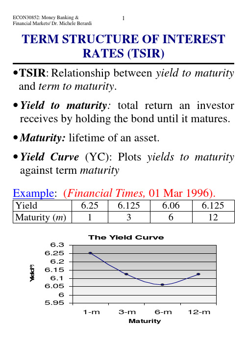
TERM STRUCTURE OF INTERESTRATES (TSIR)•T SIR:Relationship between yield to maturity and term to maturity.•Yield to maturity: total return an investor receives by holding the bond until it matures. •Maturity:lifetime of an asset.•Yield Curve(YC): Plots yields to maturity against term maturityExample: (Financial Times, 01 Mar 1996). Yield 6.25 6.125 6.06 6.125 Maturity (m) 1 3 612Other examples of Yield Curves (Financial Times, 01 Mar 1996)Euro par Yield Curve (Eurostat 5-Aug-2005)Government Bonds(zero coupon) (Bloomberg, Sun, 04 Mar 2001, 4:48pm EST) Country 3 Months 6 Months 1 yearFrance 4.670 4.570 4.530 Germany 4.761 4.651 4.535 Italy 4.235 4.539 4.432 U.K. 5.490- 5.279 U.S. 4.839 4.693 4.476U.S. Treasuries Sun, 04 Mar 2001, 5:21pm ESTBills Mat DatePreviousPrice/YieldCurrentPrice/Yield Yld Chg Prc Chg3month 5/31/01 4.71(4.83) 4.71(4.83) 0.00 -0 6month 8/30/01 4.51(4.68) 4.52(4.68) 0.01 +1 1year 2/28/02 4.26(4.46) 4.26(4.46) 0.00 +0Notes/Bonds Coupon Mat DatePreviousPrice/YieldCurrentPrice/Yield Yld Chg Prc Chg2year 4.625 2/28/03 100-10(4.46) 100-10(4.46) 0.00 -0-00 5year 5.750 11/15/05 104-09+(4.72) 104-10(4.71) 0.00 +0-00+ 10year 5.000 2/15/11 100-13+(4.95) 100-14(4.94) 0.00 +0-00+ 30year 5.375 2/15/31 100-04(5.37) 100-04+(5.37) 0.00 +0-00+InflationIndexedTreasury Coupon Mat DatePreviousPrice/YieldCurrentPrice/Yield Yld Chg Prc Chg5year 3.625 7/15/02 101-24+(2.30) 00(.00) -2.30 -101-2510year 3.500 1/15/11 101-10+(3.34) 00(.00) -3.34 -101-1130year 3.875 4/15/29 107-20(3.45) 00(.00) -3.45 -107-20TEN YEAR GOVERNMENT BOND SPREADS(Financial Times, Friday Feb 1 2008)/ft/markets/bonds.aspGov't Latest Spread vs Bund Spread vs T-Bonds N.Zealand 6.28% +2.33 +2.65 Australia 6.14% +2.19 +2.51UK 4.54% +0.59 +0.91 Norway 4.35% +0.40 +0.72 Italy 4.32% +0.37 +0.69 Greece 4.31% +0.36 +0.68 Portugal 4.22% +0.27 +0.59 Belgium 4.20% +0.25 +0.57 Austria 4.14% +0.19 +0.51 Spain 4.10% +0.15 +0.47 Denmark 4.09% +0.14 +0.46 France 4.07% +0.12 +0.44Gov't Latest Spread vs Bund Spread vs T-Bonds Finland 4.05% +0.10 +0.42 Netherlands 4.04% +0.09 +0.41 Sweden 3.97% +0.02 +0.34 Germany 3.95% 0.00 +0.32 Canada 3.90% -0.05 +0.27US 3.63% -0.32 0.00 Switzerland 2.83% -1.12 -0.80 Japan 1.43% -2.52 -2.20 Quotes are delayed by at least 20 minutes.•Compare spreads in Euro-zone with those in other countries.Government vs Corporate Bonds(Source: Baye and Jansen, 1995)•Interest rate differentials on similar assets reflect risk.UK Yield Curve (7 Feb 2009)Eurozone Yield Curve (7 Feb 2009)US Yield Curve (7 Feb 2009)Source: FT /markets/bonds.asp 08 February 20092. Main Facts of YCs: SummaryF1.YCs move together over time.F2.When short-term IRs are low, YCs slope upwards and when IRs are high YCsslope down.F3.A lmost always YCs are positive-sloping but they can also be negative-sloping(inverted) or flat.------------3. Main uses of govt. bonds YCs•YCs are used as leading indicator of economic activity/conditions.•YCs can be used as a yardstick for pricing many other fixed income securities. •YCs can be used to boost returns in bond investment strategies (known as riding the YC, or rolling down the YC).--------------4. The 3 main theories of the TSIR.A. Segmented Markets TheoryB. Expectations TheoryC. Preferred Habitat and Liquidity Theory Two important concepts•Substitutability of assets•Risk Aversion of investorsA. The Segmented Markets Theory Main assumptions/RationaleA1.Bonds of different maturities are not substitutesA2.Investors have strong preferences for bonds of particular maturities somarkets of assets are segmentedaccording to their maturity.A3.Investors prefer less risk.A4.Investors avoid transaction costs.Comments/Criticism of SMT • The SMT may explain F3.• SMT cannot explain F1 or F2.• The SMT is powerless in forecasting future rates.Maturity (years)Yield%16681210Bonds Year of Quantity −16%YieldBonds Year of Quantity −6%YieldBondsYear of Quantity −12%Yield)(Years Maturity %%8%6Bonds Year of Quantity −16%YieldBonds Year of Quantity −6%YieldBondsYear of Quantity −12%Yield )(Years Maturity %86%9B. The Expectations TheoryIan Fischer (1896), Hicks (1939) etc. … Main assumptions/RationaleA1.Investors are risk neutralA2.Short and longer-term assets are perfect substitutes.A3.No transaction costs.Given A1-A3, ET shows that longer-term rates are purely an average of expected short-term rates.Given A1-A3, decisions depend merely on the final income (V) since investors treat short and long term bonds as perfect substitutes, •With V S=V L the investor is indifferentExample On a specific date t an investor has available £1,000 for two years. On this datethe 1-year bond rate is %61=t ithe 2-year bond rate is %5.62=t i(Superscripts = term of maturity).Long-term investment22)1)(1000(£t L i V +==£1134.Short-term investmentInvestors buy the 1-year bond and re-invest their income in a second 1-year bond. (Compounded returns))1)](06.0)(1000(£1000[£11+++=t s Ei V=)1)(06.01(1000£11+++t Ei If %811=+t Ei then V S = £1144 > V L (=£1134)If %611=+t Ei then V S = £1123 < V L (=£1134).ï V S =V L due to arbitrage.The generalised formulaBased on V L =V S , we can generalise for an n-year bond (1)22)1)(1000(£t i += )1)(1(1000£111+++t t Ei i(2) 22)1(t i += )1)(1(111+++t t Ei iBased on (2) we write the general formula(3) =+n n t i )1()1)...(1)(1)(1(1112111−+++++++n t t t t Ei Ei Ei iSolving for n t i from eq. (3)(4) 1)1)...(1)(1)(1(1112111−++++=−+++n Ei Ei Ei i i n t t t t n tEquation (4) can be approximated as:(5) nEi Ei Ei i i n t t t tn t 1112111...−++++++≈(5) is used by the strict ET to explain TSIR.• It can estimate the rate that must be offered on a bond of n -years for the risk-neutral investor to hold this bond.• It can determine the shape of the yield curve. • Example : 21112++≈t t tEi i i •If short term-rates are expected to:Rise → An upward-sloping yield curve Fall → An downward-sloping yield curve Remain constant → A flat yield curve.Expectations Theory and The Yield Curve %Yield )(Years Maturity%72%)8(1112==+=+t t t Ei i i %61=t iComments and criticism of ET•The ET can explain F1, because short-term rates increase long-term rates•The ET can also explain F2, because low current short-term rates will be expected to rise in the future (and visa versa).•The ET can partially explain F3: It explains that YC can slope different ways but it implies that on average YCs should be flat. •In reality longer rates seem to under-react to changes in the short-term rate.•Unlike the SMT, the ET can be used for forecasting future interest rates.•The existence of systematic profits is totally incompatible with the ET (and part. RE).C. The Preferred Habitat and LiquidityPremium theories of TSIRMain assumptions/RationaleA1. It combines SMT and ET theories:A2. Investors are assumed to prefer one market of assets to another, but are willing to trade in other markets, given a compensation: the term premiumPreferred habitat theory (PHT) the term premium compensates for preferences.Liquidity premium theory (LPT) term premium compensates for riskBased on the ET formula, add the term nt θ.(6) nEi Ei Ei i i n t t t tn tn t 1112111...−+++++++≈θThe term premium therefore is the extra fixed yield required for the investor to be attracted into a market.• Under the SMT, only nt θ matters• Under the ET, nt θ = 0, and only expectations of short-term rates matter.Implication : Long-term IRs will equal the average of short-term IRs plus a term premiumExample: 211122+++=t t ttEi i i θ%12=t θ; %61=t i %611=+t Ei⇒ 07.0206.006.001.02=++=t iSo %61=ti and %72=t i• LPT implies an upward sloping YC,whereas under ET the YC remains flat.Comments and criticism of PHT & LPT•Both PHT and the LPT can account for allF1, F2, F3. F1 and F2 based on the ET and F3 based on the risk premium that ensuresthat on average YCs should slope upwards and allows for differences in risk premia.•Spread between L-R and S-R cannot always help predict future S-T rates.-------------。
- 1、下载文档前请自行甄别文档内容的完整性,平台不提供额外的编辑、内容补充、找答案等附加服务。
- 2、"仅部分预览"的文档,不可在线预览部分如存在完整性等问题,可反馈申请退款(可完整预览的文档不适用该条件!)。
- 3、如文档侵犯您的权益,请联系客服反馈,我们会尽快为您处理(人工客服工作时间:9:00-18:30)。
The yield curve has an upward bias built into the long-term rates because of the risk premium.
15-12
Expectations Theory
Observed long-term rate is a function of today’s short-term rate and expected future short-term rates. Long-term and short-term securities are perfect substitutes. Forward rates that are calculated from the yield on long-term securities are market consensus expected future short-term rates.
9.660 9.993
* $1,000 Par value zero
McGraw-Hill/Irwin
Copyright © 2001 by The McGraw-Hill Companies, Inc. All rights reserved.
15-7
Forward Rates from Observed Long-Term Rates
- Upward bias over expectations
Market Segmentation
- Preferred Habitat
McGraw-Hill/Irwin
Copyright © 2001 by The McGraw-Hill Companies, Inc. All rights reserved.
15-3
Yield Curves
Yields Upward Sloping Flat
Downward Sloping
Maturity
McGraw-Hill/Irwin
Copyright © 2001 by The McGraw-Hill Companies, Inc. All rights reserved.
The relationship between yield to maturity and maturity.
Information on expected future short term rates can be implied from yield curve. The yield curve is a graph that displays the relationship between yield and maturity.
(1 yn ) (1 f n ) (1 yn 1 ) n 1
n
fn = one-year forward rate for period n yn = yield for a security with a maturity of n
(1 yn ) (1 yn1 ) (1 f n )
McGraw-Hill/Irwin
Copyright © 2001 by The McGraw-Hill Companies, Inc. All rights reserved.
15-1
Chapter 15
The Term Structure of Interest Rates
McGraw-Hill/Irwin
Copyright © 2001 by The McGraw-Hill Companies, Inc. All rights reserved.
15-2
Overview of Term Structure of Interest Rates
=
=
0.063336
0.063008
Copyright © 2001 by The McGraw-Hill Companies, Inc. All rights reserved.
15-11
Theories of Term Structure
Expectations
Liquidity Preference
McGraw-Hill/Irwin
Copyright © 2001 by The McGraw-Hill Companies, Inc. All rights reserved.
15-13
Liquidity Premium Theory
Long-term bonds are more risky.
PVn = Present Value of $1 in n periods r1 = One-year rate for period 1
r2 = One-year rate for period 2
rn = One-year rate for period n
McGraw-Hill/Irwin
Copyright © 2001 by The McGraw-Hill Companies, Inc. All rights reserved.
McGraw-Hill/Irwin
Copyright © 2001 by The McGraw-Hill Companies, Inc. All rights reserved.
15-10
Forward Rates for Downward Sloping Yield Curve
1yr Forward Rates
15-14
Liquidity Premiums and Yield Curves
Yields
Observed Yield Curve
Forward Rates
Liquidity Premium Maturity
McGraw-Hill/Irwin
Copyright © 2001 by The McGraw-Hill Companies, Inc. All rights reserved.
McGraw-Hill/Irwin
Copyright © 2001 by The McGraw-Hill Companies, Inc. All rights reserved.
15-17
Using Spot Rates to Price Coupon Bonds
A coupon bond can be viewed as a series of zero coupon bonds. To find the value each payment is discount at the zero coupon rate. Once the bond value is found, one can solve for the yield. It’s the reason that similar maturity and default risk bonds sell at different yields to maturity.
McGraw-Hill/Irwin
Copyright © 2001 by The McGraw-Hill Companies, Inc. All rights reserved.
15-9
Downward Sloping Spot Yield Curve
Zero-Coupon Rates Bond Maturity 12% 1 11.75% 2 11.25% 3 10.00% 4 9.25% 5
Forward rates contain a liquidity premium and are not equal to expected future short-term rates.
McGraw-Hill/Irwin
Copyright © 2001 by The McGraw-Hill Companies, Inc. All rights reserved.
Copyright © 2001 by The McGraw-Hill Companies, Inc. All rights reserved.
15-5
Pricing of Bonds using Expected Rates
1 PVn (1 r1 ) (1 r2 )...(1 rn )
15-15
Liquidity Premiums and Yield Curves
Yields
Observed Yield Curve
Forward Rates Liquidity Premium
Maturity
McGraw-Hill/Irwin
Copyright © 2001 by The McGraw-Hill Companies, Inc. All rights reserved.
Three major theories are proposed to explain the observed yield curve.
McGraw-Hill/Irwin
Copyright © 2001 by The McGraw-Hill Companies, Inc. All rights reserved.
3yr = 9.660
fn = ?
(1.0993)4 = (1.0966)3 (1+fn) (1.46373) / (1.31870) = (1+fn) fn = .10998 or 11% Note: this is expected rate that was used in the prior example.