[宏观经济学第12讲_短期权衡取舍
高鸿业《宏观经济学》第十二章国民收入核算

•克林顿的实际年薪 :
•
二、潜在GDP:木桶的最大容量
1、含义:一国一定时期内可供利用的生产资源(L、K、N) 在正常情况下可以生产的最大产量。
2、公式: GDP*=Л*×(L*×H*) 其中, Л*——每人每小时的平均产值, L*——充分就业时的就业人数, H*——就业者在一年内每人劳动的小时数 而GDP= Л*×(L×H*) 其中, L——实际就业人数
最终产品的总卖价来计算GDP. 理解要点:谁购买?各支出多少?
1、GDP的构成:GDP=C+I+G+(X-M)
•
2、详解
(1)居民个人消费支出:consumption 指的是居民对最终消费品的支出。包括购买耐用
品、非耐用品和劳务的支出。 它构成一个国家总支出中一个主要部分(2/3)
•我买的新 房子是不 是消费支
(二)与PI牵手:DPI=PI-个人所得税 (三)构成:DPI=C+S,C=DPI-S
•
第四节 国民收入基本公式
——宏观经济模型
总方针:支出=收入,无论用什么方法核算,支出应等于收
入
一、两部门模型
1、主角:居民户 厂商 2、支出=C+I, 3、收入=C+S,所以有恒等式I=S
二、三部门模型
得 (1)I+(X-M-Kr)=S+(T-G),表示私人国内
总投资+可支配的外国资产=私人储蓄+政府储 蓄; (2)I=S+(T-G)+(M-X+Kr),表示投资=私 人储蓄+政府储蓄+国外储蓄
•
第五节 名义GDP与实际GDP
一、名义与实际GDP
(一)名义GDP(Nominal GDP)
《经济学原理:短期经济波动》

第35章 通货膨胀与失业之间的短期权衡取舍
一.菲利普斯曲线 1. 菲利普斯曲线的由来 2. 总需求、总供给和菲利普斯曲线 菲利普斯曲线说明,短期中出现的通货膨胀与失 业的组合是由于总需求曲线的移动使经济沿着短 期总供给曲线变动; 因为货币政策与财政政策可以使总需求曲线移 动,所以它们可以使经济沿着菲利普斯曲线移 动;
货币供给
物价水平
总需求 AD1
AD2
r1
2,支出增加 货币需求
MD2
r2 1,政府购买
AD3
4,挤出效应部分抵消 了总需求的增加
上
升0
MD1
央行固定货币量
货币量
增加总需求
0
产量
图:挤出效应
第34章 货币政策与财政政策对总需求的影响
6. 税收变动 减税增加了消费支出,就会使总需求曲线向右移动,同样,增税抑制了消费支出,使总需求曲线向左移 动;
物价水平
长期总供给
P1 物价水
平变动 P2
不影响长期中物品与 服务的供给量
0
自然水平
产量
图:总需求曲线
物价水平
LRAS1990 LRAS2000 LRAS2010
货币供给增长 总需求曲线移动
技术进步使长期 总供给曲线移动
P2010
持续的通货 膨胀
P2000
P1990
AD1990
AD2010 AD2000
二.运用政策来稳定经济 1. 支持积极稳定政策论 凯恩斯(及其许多追随者)认为,总需求的波动主要是因为非理性的悲观主义者与乐观主义者; 从原则上说,政府可以调整货币政策与财政政策以对这些乐观主义和悲观主义情绪做出反应,从而稳 定经济; 2. 反对积极稳定政策论 反对者认为:货币政策和财政政策有时滞; 3. 自动稳定器 ① 最重要的自动稳定器是税制; ② 政府支出也作为自动稳定器发挥作用;
2023版经济学原理名词解释
2023版经济学原理名词解释第一章1.稀缺性:社会拥有的资源是有限的,因此不能生产人们希望用油的所有物品与劳务2.经济学:研究社会如何管理自己的稀缺资源3.效率:社会能从稀缺资源中得到的最大利益4.平等:讲这些资源的成果平均地分配给社会成员5.机会成本:为了得到这种东西所放弃的东西6.理性人:能系统而由母的的尽最大努力去实现目标7.编辑变动:对现有行动计划的微小增量调整8.激励:引起一个人做出某种行为的某种东西9.市场失灵:市场本身不能有效配置资源的情况10.外部性:一个人的行为对旁观者福利的影响11.市场势力:单个人或者一小群人不适当地影响市场价格的能力12.生产率:每一单位劳动投入所生产的物品与劳动数量经济学十大原理1.人们面临权衡取舍2、某种东西的成本是为了得到它所放弃的东西3、理性人考虑边际量4、人们会对激励做出反应5、毛衣可以使每个人的状况都变得更好6、市场通常是组织经济活动的一种好方法7、政府又是可以改善市场结果8、一国的生活水平取决于它生产物品与劳务的能力9、当政府发行了过多的货币时,物价上升10、社会面临通货膨胀与事业之间的短期权衡取舍第二章要点1.循环流向图,见书20o在这个模型中,经济由两类觉得这,家庭和企业组成,2.物品与劳务市场上,家庭是买者,生产要素市场上,家庭是卖者3.生产可能性边界:一个图形,标明在生产要素和生产技术既定时,一个经济所能生产的产出。
大炮与黄油4.微观经济学:研究家庭和企业如何做出决策,以及他们如何在特定市场上相互影响5.宏观经济学:研究整体经济现象6.关于世界的表述有两种类型:一,实证表述:描述性的,关于世界是什么样子的表述;二,规范表述:关于世界应该是什么样子的表述第四章供给与需求的市场力量1.某种物品与劳务的买者与卖者组成的一个群体2、竞争市场:有许多买者与卖者,以至于一个人对市场价格的影响微乎其微的市场3、完全竞争的市场具有的两个特征:可供销售的物品是完全相同的;买者与卖者众多以至于任何一个买者或卖者无法影响市场价格,此时他们被称为价格接受者4、垄断者:一些市场只有一个卖者,由他决定价格5.需求量:买者愿意并且能够购买的该种物品的数量6.需求定理:在其他条件不变的情况下,价格上升,该物品的需求量减少,价格下降,需求量增加7.需求曲线:把价格与需求量联系一起的向右下方倾斜的曲线8.市场需求:所有个人对某种特定物品或劳务的需求的总和9.需求变动:需求曲线向右移动为去求增加,向左移动为需求减少10.影响需求量的因素:价格11.影响需求的因素:收入,相关物品的价格,嗜好,预期,买者数量12.供给量:卖者愿意并且能够出售的该种物品的数量13.供给定理:在其他条件不变时,一种物品价格上升,该物品的供给量增加,一种物品价格下降,该物品供给量减少14.供给变动:供给曲线向右移动,为供给增加,供给曲线向左移动,为供给减少15.影响供给的因素:投入品的价格,技术,预期,卖者数量16.分析均衡变动的三个步骤:一,确定该事件是使供给曲线移动还是使需求曲线移动,还是两者都移动;二,确定曲线移动方向;三。
经济学原理 (12.5)--通货膨胀与失业之间的短期权衡取舍、宏观经济政策的六个争论问题-习题答案
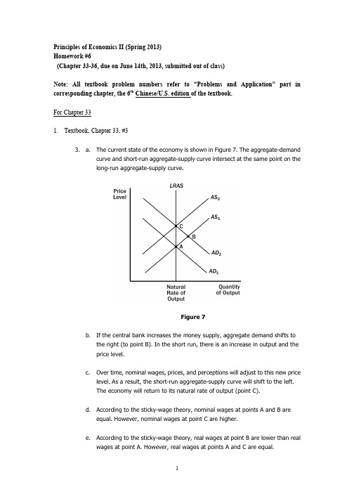
Principles of Economics II (Spring 2013)Homework #6(Chapter 33-36, due on June 14th, 2013, submitted out of class)Note: All textbook problem numbers refer to “Problems and Application” part in corresponding chapter, the 6th Chinese/U.S. edition of the textbook.For Chapter 331.Textbook, Chapter 33, #33. a. The current state of the economy is shown in Figure 7. The aggregate-demandcurve and short-run aggregate-supply curve intersect at the same point on thelong-run aggregate-supply curve.Figure 7b. If the central bank increases the money supply, aggregate demand shifts tothe right (to point B). In the short run, there is an increase in output and theprice level.c. Over time, nominal wages, prices, and perceptions will adjust to this new pricelevel. As a result, the short-run aggregate-supply curve will shift to the left.The economy will return to its natural rate of output (point C).d. According to the sticky-wage theory, nominal wages at points A and B areequal. However, nominal wages at point C are higher.e. According to the sticky-wage theory, real wages at point B are lower than realwages at point A. However, real wages at points A and C are equal.f. Yes, this analysis is consistent with long-run monetary neutrality. In the longrun, an increase in the money supply causes an increase in the nominal wage,but leaves the real wage unchanged.2.Textbook, Chapter 33, # 55. a. The statement that "the aggregate-demand curve slopes downward because itis the horizontal sum of the demand curves for individual goods" is false. Theaggregate-demand curve slopes downward because a fall in the price levelraises the overall quantity of goods and services demanded through the wealtheffect, the interest-rate effect, and the exchange-rate effect.b. The statement that "the long-run aggregate-supply curve is vertical becauseeconomic forces do not affect long-run aggregate supply" is false. Economicforces of various kinds (such as population and productivity) do affect long-runaggregate supply. The long-run aggregate-supply curve is vertical because theprice level does not affect long-run aggregate supply.c. The statement that "if firms adjusted their prices every day, then the short-runaggregate-supply curve would be horizontal" is false. If firms adjusted pricesquickly and if sticky prices were the only possible cause for the upward slope ofthe short-run aggregate-supply curve, then the short-run aggregate-supplycurve would be vertical, not horizontal. The short-run aggregate supply curvewould be horizontal only if prices were completely fixed.d. The statement that "whenever the economy enters a recession, its long-runaggregate-supply curve shifts to the left" is false. An economy could enter arecession if either the aggregate-demand curve or the short-runaggregate-supply curve shifts to the left.3.Textbook, Chapter 33, # 88. a. People will likely expect that the new chairman will not actively fight inflationso they will expect the price level to rise.b. If people believe that the price level will be higher over the next year, workerswill want higher nominal wages.c. At any given price level, higher labor costs lead to reduced profitability.d. The short-run aggregate-supply curve will shift to the left as shown in Figure10.Figure 10e. A decline in short-run aggregate supply leads to reduced output and a higherprice level.f. No, this choice was probably not wise. The end result is stagflation, whichprovides limited choices in terms of policies to remedy the situation.Figure 114.Textbook, Chapter 33, # 99. a. If households decide to save a larger share of their income, they must spendless on consumer goods, so the aggregate-demand curve shifts to the left, as shown in Figure 11. The equilibrium changes from point A to point B, so theprice level declines and output declines.b. If Florida orange groves suffer a prolonged period of below-freezingtemperatures, the orange harvest will be reduced. This decline in the naturalrate of output is represented in Figure 12 by a shift to the left in both theshort-run and long-run aggregate-supply curves. The equilibrium changesfrom point A to point B, so the price level rises and output declines.Figure 12Figure 13c. If increased job opportunities cause people to leave the country, the long-runand short-run aggregate-supply curves will shift to the left because there arefewer people producing output. The aggregate-demand curve will also shift tothe left because there are fewer people consuming goods and services. Theresult is a decline in the quantity of output, as Figure 13 shows. Whether theprice level rises or declines depends on the relative sizes of the shifts in theaggregate-demand curve and the aggregate-supply curves.5.Textbook, Chapter 33, #1111. a. If firms become optimistic about future business conditions and increaseinvestment, the result is shown in Figure 18. The economy begins at point Awith aggregate-demand curve AD1 and short-run aggregate-supply curve AS1.The equilibrium has price level P1 and output level Y1. Increased optimismleads to greater investment, so the aggregate-demand curve shifts to AD2.Now the economy is at point B, with price level P2 and output level Y2. Theaggregate quantity of output supplied rises because the price level has risenand people have misperceptions about the price level, wages are sticky, orprices are sticky, all of which cause output supplied to increase.Figure 18b. Over time, as the misperceptions of the price level disappear, wages adjust, orprices adjust, the short-run aggregate-supply curve shifts up to AS2 and theeconomy gets to equilibrium at point C, with price level P3 and output level Y1.The quantity of output demanded declines as the price level rises.c. The investment boom might increase the long-run aggregate-supply curvebecause higher investment today means a larger capital stock in the future,thus higher productivity and output.6.Textbook, Chapter 33, # 1212. Economy B would have a more steeply sloped short-run aggregate-supply curvethan would Economy A, because only half of the wages in Economy B are “sticky.”A 5% increase in the money supply would have a larger effect on output inEconomy A and a larger effect on the price level in Economy B.7.True or false? Keynes's primary message in The General Theory was that short-run economicfluctuations were the result of inadequate aggregate demand that could be corrected by using government policy.TrueFor Chapter 348.Textbook, Chapter 34, # 11. a. When the Fed’s bond traders buy bonds in open-market operations, themoney-supply curve shifts to the right from MS1 to MS2, as shown in Figure 1.The result is a decline in the interest rate.Figure 1 Figure 2b. When an increase in credit card availability reduces the cash people hold, themoney-demand curve shifts to the left from MD1 to MD2, as shown in Figure 2.The result is a decline in the interest rate.c. When the Federal Reserve reduces reserve requirements, the money supplyincreases, so the money-supply curve shifts to the right from MS1 to MS2, asshown in Figure 1. The result is a decline in the interest rate.d. When households decide to hold more money to use for holiday shopping, themoney-demand curve shifts to the right from MD1 to MD2, as shown in Figure3. The result is a rise in the interest rate.Figure 3e. When a wave of optimism boosts business investment and expands aggregatedemand, money demand increases from MD1 to MD2 in Figure 3. The increasein money demand increases the interest rate.Figure 49.Textbook, Chapter 34, # 22. a. The increase in the money supply will cause the equilibrium interest rate todecline, as shown in Figure 4. Households will increase spending and willinvest in more new housing. Firms too will increase investment spending. Thiswill cause the aggregate demand curve to shift to the right as shown in Figure5.Figure 5b. As shown in Figure 5, the increase in aggregate demand will cause an increasein both output and the price level in the short run (point B).c. When the economy makes the transition from its short-run equilibrium to itslong-run equilibrium, short-run aggregate supply will decline, causing the pricelevel to rise even further (point C).d. The increase in the price level will cause an increase in the demand for money,raising the equilibrium interest rate.e. Yes. While output initially rises because of the increase in aggregate demand,it will fall once short-run aggregate supply declines. Thus, there is no long-runeffect of the increase in the money supply on real output.10.Textbook, Chapter 34, # 3Figure 63. a. When fewer ATMs are available, money demand is increased and themoney-demand curve shifts to the right from MD1 to MD2, as shown in Figure6. If the Fed does not change the money supply, which is at MS1, the interestrate will rise from r1 to r2. The increase in the interest rate shifts theaggregate-demand curve to the left, as consumption and investment fall.b. If the Fed wants to stabilize aggregate demand, it should increase the moneysupply to MS2, so the interest rate will remain at r1 and aggregate demand willnot change.c. To increase the money supply using open market operations, the Fed shouldbuy government bonds.11.Textbook, Chapter 34, #88. a. The initial effect of the tax reduction of $20 billion is to increase aggregatedemand by $20 billion × 3/4 (the MPC) = $15 billion.b. Additional effects follow this initial effect as the added incomes are spent. Thesecond round leads to increased consumption spending of $15 billion × 3/4 =$11.25 billion. The third round gives an increase in consumption of $11.25billion × 3/4 = $8.44 billion. The effects continue indefinitely. Adding them allup gives a total effect that depends on the multiplier. With an MPC of 3/4, themultiplier is 1/(1 – 3/4) = 4. So the total effect is $15 billion × 4 = $60 billion.c. Government purchases have an initial effect of the full $20 billion, becausethey increase aggregate demand directly by that amount. The total effect of anincrease in government purchases is thus $20 billion × 4 = $80 billion. Sogovernment purchases lead to a bigger effect on output than a tax cut does.The difference arises because government purchases affect aggregatedemand by the full amount, but a tax cut is partly saved by consumers, andtherefore does not lead to as much of an increase in aggregate demand.d. The government could increase taxes by the same amount it increases itspurchases.12.Textbook, Chapter 34, # 99. If the marginal propensity to consume is 0.8, the spending multiplier will be 1/(1 – 0.8) = 5. Therefore, the government would have to increase spending by $400/5 = $80 billion to close the recessionary gap.13.Textbook, Chapter 34, 1111. a. Expansionary fiscal policy is more likely to lead to a short-run increase ininvestment if the investment accelerator is large. A large investmentaccelerator means that the increase in output caused by expansionary fiscalpolicy will induce a large increase in investment. Without a large accelerator,investment might decline because the increase in aggregate demand will raisethe interest rate.b. Expansionary fiscal policy is more likely to lead to a short-run increase ininvestment if the interest sensitivity of investment is small. Because fiscalpolicy increases aggregate demand, thus increasing money demand and theinterest rate, the greater the sensitivity of investment to the interest rate thegreater the decline in investment will be, which will offset the positiveaccelerator effect.For Chapter 3514.Textbook, Chapter 35, #11. Figure 8 shows two different short-run Phillips curves depicting these four points.Points A and D are on SRPC1 because both have expected inflation of 3%. Points Band C are on SRPC2 because both have expected inflation of 5%.Figure 815.Textbook, Chapter 35, #4Figure 144. a. Figure 14 shows the economy in long-run equilibrium at point A, which is onboth the long-run and short-run Phillips curves.b. A wave of business pessimism reduces aggregate demand, moving theeconomy to point B in the figure. The unemployment rate rises and theinflation rate declines. If the Fed undertakes expansionary monetary policy, itcan increase aggregate demand, offsetting the pessimism and returning theeconomy to point A, with the initial inflation rate and unemployment rate.c. Figure 15 shows the effects on the economy if the price of imported oil rises.The higher price of imported oil shifts the short-run Phillips curve up fromSRPC1 to SRPC2. The economy moves from point A to point C, with a higherinflation rate and higher unemployment rate. If the Fed engages inexpansionary monetary policy, it can return the economy to its originalunemployment rate at point D, but the inflation rate will be higher. If the Fedengages in contractionary monetary policy, it can return the economy to itsoriginal inflation rate at point E, but the unemployment rate will be higher. Thissituation differs from that in part (b) because in part (b) the economy stayedon the same short-run Phillips curve, but in part (c) the economy moved to ahigher short-run Phillips curve, which gives policymakers a less favorabletrade-off between inflation and unemployment.Figure 1516.Textbook, Chapter 35, #6Figure 166. If the Fed acts on its belief that the natural rate of unemployment is 4%, when thenatural rate is in fact 5%, the result will be a spiraling up of the inflation rate, asshown in Figure 16. Starting from a point on the long-run Phillips curve, with anunemployment rate of 5%, the Fed will believe that the economy is in a recession,because the unemployment rate is greater than its estimate of the natural rate.Therefore, the Fed will increase the money supply, moving the economy along theshort-run Phillips curve SRPC1. The inflation rate will rise and the unemploymentrate will fall to 4%. As the inflation rate rises over time, expectations of inflationwill rise, and the short-run Phillips curve will shift up to SRPC2. This process willcontinue, and the inflation rate will spiral upwards.The Fed may eventually realize that its estimate of the natural rate ofunemployment is wrong by examining the rising trend in the inflation rate.17.Textbook, Chapter 35, #77. a. If wage contracts have short durations, a recession induced by contractionarymonetary policy will be less severe, because wage contracts can be adjustedmore rapidly to reflect the lower inflation rate. This will allow a more rapidmovement of the short-run aggregate-supply curve and short-run Phillipscurve to restore the economy to long-run equilibrium.b. If there is little confidence in the Fed's determination to reduce inflation, arecession induced by contractionary monetary policy will be more severe. Itwill take longer for people's inflation expectations to adjust downwards.c. If expectations of inflation adjust quickly to actual inflation, a recessioninduced by contractionary monetary policy will be less severe. In this case,people's expectations adjust quickly, so the short-run Phillips curve shiftsquickly to restore the economy to long-run equilibrium at the natural rate ofunemployment.18.Textbook, Chapter 35, #9Figure 179. a. As shown in the left diagram of Figure 17, equilibrium output and employmentwill fall. However, the effects on the price level and inflation rate will beambiguous. The fall in aggregate demand puts downward pressure on prices,while the decline in short-run aggregate supply pushes prices up. The diagramon the right side of Figure 17 assumes that the inflation rate rises.b. The Fed would have to use expansionary monetary policy to keep output andemployment at their natural rates. Aggregate demand would have to shift toAD3.c. The Fed may not want to pursue this action because it will lead to a rise in theinflation rate as shown by point C.19.选举周期与经济波动:一个经济某一年的菲利普斯曲线由下列的关系式确定:π = πe - (u - 4%)。
宏观经济学(高鸿业版)第12章重点总结

宏观经济学(高鸿业版)第12章重点总结第一篇:宏观经济学(高鸿业版)第12章重点总结第十三章简单国民收入决定理论1.均衡产出:是和总需求相一致的产出,也就是经济社会的收入正好等于全体居民和企业想要有的产出。
简单的说就是和总需求相等的产出或收入。
2.均衡产出的条件:E=y 也可以用 i=s来表示。
3.消费函数:消费与可支配收入之间的依存关系。
c=c(y)c=α+βy4.边际消费倾向MPC:增加的消费与增加的收入之比率,也就是增加的1单位收入中用于增加消费部分的比率。
MPC=△c/△y =dc/dy5.平均消费倾向APC:指任一收入水平上消费之支出在收入中的比率。
APC=c/y6.储蓄函数:指储蓄与决定储蓄的各种因素之间的依存关系。
(广义)7.储蓄函数方程式: s=y-c=y-(α+βy)=-α+(1-βy)8.消费函数和储蓄函数的关系 P3879.均衡收入:y=(α+ I)/(1-β)P39310.投资乘数:指收入的变化与带来这种变化的投资支出的变化的比率。
k=1/(1-β)11.三部门经济中各种乘数 P399第十四章产品市场和货币市场的一般均衡1.资本边际效率MEC : 是一种贴现率,这种贴现率正好使一项资本物品的使用期内各预期收益的现值之和等于这项资本品的供给价格或者重置成本。
(公式P412)2.IS曲线:一条反应利率和收入间相互关系的曲线。
这条曲线上任何一点都代表一定的利率和收入的组合,在这些组合下,投资和储蓄都是相等的,即I=S,从而产品市场是均衡的。
3.货币需求动机:1)交易动机:指个人和企业需要货币是为了进行正常的交易活动。
收入越高,交易数量越大,为应付日常开支所需的货币量就越大。
2)谨慎动机(预防性动机):指为预防意外支出而持有一部分货币的动机,货币需求量大体上和收入成正比。
3)投机动机:指人们为了抓住有利的购买有价证券的机会而持有一部分货币的动机。
4.流动偏好陷阱:当利率极低,人们认为这时利率不大可能再下降,或者说有价证券市场价格不大可能再上升而只会跌落,人们不管有多少货币都愿意持在手中。
高鸿业五版宏观经济学第12章.ppt

2.宏观经济学运用经济加总法时值得注意的几点 第一,宏观分析中有些总量变化可以从微观分析 的个量中直接加总(大部分是加权平均加总)而 得到。
2019年3月30日星期六 制作者:勤奋之人工作室 24
第十二章 国民收入核算 第一节 宏观经济学的特点
2.宏观经济学运用经济加总法时值得注意的几点 第二,有的时候微观经济学中一些个体变量尽管 可以加总,但是这种加总却达不到研究整个社会 经济行为的目的。 尽管微观是宏观的基础,但总体经济行为并不 是个体经济行为的简单加总。对微观经济是正确 的东西,对宏观经济未必也是正确的。
2019年3月30日星期六
制作者:勤奋之人工作室
20
第十二章 国民收入核算 第一节 宏观经济学的特点
2.宏观宏观经济学与微观经济学的主要相同之处 第一,微观经济学中的价格和产量是一个个具体 商品的价格和产量——个量,而宏观经济学中的 价格和产量是整个社会的价格水平和产出水平— —总量,这里价格水平用价格指数表示,产出水 平用货币衡量的市场价值(国内生产总值)表示。
第十二章 国民收入核算 第一节 宏观经济学的特点
3.测度宏观经济运行情况的重要指标 第三,物价水平 物价水平指物价总水平,一般用价格指数即 社会上若干种商品价格水平的指数来表示。价格 指数包括消费物价措数(CPI)、生产者价格指数 (PPI)以及GDP折算指数三种。 物价水平的变动用通货膨胀率表示。
2019年3月30日星期六 制作者:勤奋之人工作室 21
第十二章 国民收入核算 第一节 宏观经济学的特点
2.宏观宏观经济学与微观经济学的主要相同之处 第二,微观经济学中需求曲线和供给曲线的一般 形态,看起来和宏观经济学中的总需求曲线和短 期总供给曲线的形态都差不多地向右下方倾斜和 向右上方倾斜,但是其原因却是不同的。
宏观经济学(第12章)(高鸿业版)

PPT课件
19
第十二章 国民收入核算 National income accounting
本章学习目的
1.掌握国内生产总值(GDP)的概念及其局限性 2.掌握国民收入核算中的恒等关系 3.熟悉国民收入核算的两种基本方法 4.熟悉宏观经济总量之间的数量增减关系
总收入:GDP=Y=要素收入之和=工资 +利息+地租+利润=消费(C)+储蓄(S)
C+I=C+S
I=S
PPT课件
36
第二节 产出、收入、支出
2.三部门经济国民收入流量循环
总支出:GDP=Y=消费需求+投资需求+政府需求 =C+I+G
总体行为 宏观最优化 宏观均衡 微观基础
总产量 总收入 总支出
恒等式
S=I
宏观分析
宏观经济 循环流转
宏观分析
结
构 PPT课件
产品市场 要素市场 货币市场 国外市场
长期分析
家庭 政府 部门 厂商
17
宏观经济分析的基础(续)
恒等式 S=I
宏观分析 结构
S+T=I+G
S+T+M=I+G+X
长期分析 短期分析
1.名义国内生产总值(nominal GDP)是用当期的产量乘当
期的价格计算出来的GDP。
2.实际国内生产总值(real GDP)是用当期的产量乘基期的
价格计算出来的GDP。
名义GDP
3.国内生产总值价格指数=
×100%
(GDP price index)
实际GDP
[经济学]第35章 通货膨胀和失业之间的短期权衡取舍
![[经济学]第35章 通货膨胀和失业之间的短期权衡取舍](https://img.taocdn.com/s3/m/02b01b01680203d8ce2f24da.png)
[经济学]第35章通货膨胀和失业之间的短期权衡取舍第三十五章通货膨胀与失业之间的短期权衡,菲利普斯曲线,菲利普斯曲线运动:预期效应,通货膨胀与失业之间的短期权衡,菲利普斯曲线运动:供给冲击,降低通货膨胀成本,结论,顺序,执行摘要,菲利普斯曲线描述了通货膨胀与失业之间的负相关关系。
与此同时,降低失业率的政策导致了更高的通货膨胀率以及通货膨胀与失业之间的负相关。
只有在短期内,不利的供应冲击才会改变短期菲利普斯曲线。
当美联储收紧货币供应以降低通货膨胀时,它将使经济沿着短期菲利普斯曲线运行,这将导致暂时的高失业率。
反通胀的成本取决于通胀预期的下降速度。
一些经济学家认为,可信的低通胀承诺可以通过调整预期来降低反通胀成本。
通货膨胀和失业之间的短期权衡。
依次,通货膨胀和失业是人们经常关心的两个指标。
一些经济学家称通货膨胀率和失业率之和为社会的“痛苦指数”。
从长远来看,最低工资法、工会力量、效率工资和求职的有效性决定了失业率。
货币供应量的增长决定了通货膨胀率。
短期内情况完全不同。
当决策者使用财政或货币政策来扩大总需求时,他们可以在短期内扩大产出并降低失业率,但这会导致价格快速上涨。
当决策者采取紧缩的财政或货币政策时,通货膨胀和失业之间的短期权衡可以在短期内减少,但代价是暂时的低产出和高失业率。
在本章中,我们将进一步研究通货膨胀和失业之间的短期权衡。
1958年,英国经济学家菲利普斯首次发现了通货膨胀和失业之间的负相关关系(当时他用名义工资的变化来表示通货膨胀)。
两年后,美国经济学家萨缪尔森(Samuelson)和索洛(Solow)用美国数据显示了通胀和失业之间的负相关性。
此外,得出的结论是,这种相关性是由于低失业率和高总需求之间的相关性。
两人指出,菲利普斯曲线为决策者提供了一个可能的经济结果菜单。
通过改变货币或财政政策,决策者可以选择曲线上的任何一点,通货膨胀和失业之间的短期权衡,菲利普斯曲线和菲利普斯曲线为决策者提供了一个可能的经济结果菜单。
- 1、下载文档前请自行甄别文档内容的完整性,平台不提供额外的编辑、内容补充、找答案等附加服务。
- 2、"仅部分预览"的文档,不可在线预览部分如存在完整性等问题,可反馈申请退款(可完整预览的文档不适用该条件!)。
- 3、如文档侵犯您的权益,请联系客服反馈,我们会尽快为您处理(人工客服工作时间:9:00-18:30)。
石油价格上涨 每桶原油价格:2004年2月的35美元到2008年6月的134 美元 从2007年6月到2008年6月:
失业率从4.6%上升到 5.5% CPI通货膨胀率从2.6%上升到4.9%
Page 29
结论
本章的理论是20世纪许多最优秀的经济学家的思想
他们告诉我们通货膨胀与失业率:
1960年,保罗· 萨缪尔森(Paul Samuelson)与罗伯特· 索 洛(Robert Solow)发现美国通货膨胀与失业之间也存在 这种负相关关系,他们把它称为“菲利普斯曲线”
Page 3
菲利普斯曲线的推导
假设今年 P = 100
下面的图形表示明年可能出现的两种结果:
A.总需求低,物价水平上升缓慢(低通货膨胀), 低产出,高失业 B. 总需求高,物价水平上升快(高通货膨胀), 高产出,低失业
罗伯特· 卢卡斯(Robert Lucas),托马斯· 萨金特
(Thomas Sargent),罗伯特· 巴罗(Robert Barro) 意味着反通货膨胀的成本可能要小得多……
Page 23
理性预期与无代价地反通货膨胀
如果联储向每个人做出降低通货膨胀的可信承诺 那预期通货膨胀会下降,短期菲利普斯曲线向下移动 结果:反通货膨胀引起的失业比传统牺牲率估计的要小
通货膨胀率 (年百分比)
10 8
6 4 2 0 0 2 4
20世纪70年代初期:虽然 通货膨胀率很高,失业率 还是在上升 费里德曼和菲 利普斯解释: 人们对通货膨 73 胀的预期赶上 71 69 70 68 了现实 72
66 67 65 64 63 62 1961
6
Page 15
8
10 失业率 (百分比)
4 2 0 0 2 4
2000
05 06 96 02 94 1987
92
98
6
Page 28
8
10 失业率 (百分比)
伯南克的挑战
总需求冲击:
次贷危机,住房价格下降,大量丧失赎权,金融机构处于 困境
总供给冲击:
食品/农产品价格上涨,如每蒲式耳玉米的价格从20052006年的2.10美元上涨到2008年5月的5.76美元
1972
8
10 失业率 (百分比)
降低通货膨胀的代价
反通货膨胀:降低通货膨胀率
为降低通货膨胀率,美联储必须降低货币增长率,以减少 总需求
短期:产出下降,失业上升 长期:产出与失业回到各自的自然率水平
Page 20
反通货膨胀的货币政策
紧缩性货币政策使经济从A
点移到B点
随着时间的推移, 预期通货膨胀下降,菲利 普斯曲线向下移动 在长期中,经济回到
Page 8
垂直的长期菲利普斯曲线
在长期中,货币增长越快只会导致通货膨胀率越高
P
LRAS 通货膨 胀 高通 胀 LRPC
P2
P1
AD2 AD1 Y
低通 胀 失业率 自然失业率
9
自然产量率
使理论与证据一致
来自20世纪60年代的证据: 菲利普斯曲线向右下方倾斜 理论(弗里德曼与费尔普斯): 长期菲利普斯曲线是垂直的 为使理论与证据相一致,弗里德曼与费尔普斯引进了一个 新的变量:预期通货膨胀 – 衡量人们预期物价总水平的变 动幅度
在长期中是无关的 短期中是负相关的 受预期影响,预期在经济从短期向长期调整过程中起着相当重要的 作用
Page 30
内容提要
菲利普斯曲线描述了通货膨胀与失业之间的短期权衡取舍
在长期中,通货膨胀与失业之间并不存在权衡取舍:通货
膨胀率取决于货币增长率,而失业率等于自然失业率 供给冲击与预期通货膨胀的变动会使短期菲利普斯曲线发 生移动,从而给决策者一个更有利或不利的通货膨胀和失 业之间的权衡取舍
结果: 高预期通货膨胀使菲利普斯曲线 进一步向右移动 1979年,石油价格再次上涨,联 储面临更艰难的权衡取舍
Page 18
20世纪70年代的石油价格冲击
通货膨胀率 (年百分比)
10 8
6 4 2 0 0 2 4 6
Page 19
81 75 74 79 78 73 77 76 80
供给冲击和 预期通货膨 胀率的上升 使联储面临 更艰难的权 衡取舍
通货膨胀率主要取决于货币供给的增长率
自然失业率取决于最低工资法,工会的市场势力,效率工资以及寻 找工作的有效性
经济学十大原理之一: 社会面临通货膨胀和失业之间的短期权衡取舍
Page 2
菲利普斯曲线
菲利普斯曲线:一条表示通货膨胀与失业之间短期权衡取 舍的曲线 1958年,菲利普斯(A.W. Phillips)说明英国名义工资增 长率与失业率之间的负相关关系
过程
13
主动学习 1
参考答案
PCB
LRPCD
LRPCA
7 6
inflation rate
预期通货膨 胀率的上升 使菲利普斯 曲线向右移 动 自然失业率 的下降使两 条曲线都向 左移动
5 4 3 2 1 0 0 1 2 3 4 5 6 7 8
14
PCD PCC
unemployment rate
菲利普斯曲线的破灭
A
PC2 PC1
失业率
AD Y2
Y1
Y
随着菲利普斯曲线向右移动,通货膨胀率与失业率都上升
Page 17
20世纪70年代的石油价格冲击
每桶原油价格 1/1973 1/1974 1/1979 1/1980 1/1981 $ 3.56 10.11 14.85 32.50 38.00
美联储用更快的货币增长来抵消 1973年的第一次石油价格冲击
Page 25
沃尔克的反通货膨胀
通货膨胀率 (年百分比)
10
80
反通货膨胀的代价非常高
81
8
6 4
1979 82 84 83 87 85 86
在1982-1983 年,失业率接 近10%
2 0 0 2 4 6
Page 26
8
10 失业率 (百分比)
格林斯潘时代
1986年:石油价格下降了50% 1989 -1990年: 失业率下降,通货膨胀上升,美联 储提高利率,引起经济的微小衰退 格林斯潘 联邦公开市场委 员会主席 1987.8-2006.1
20世纪90年代:
失业率和通货膨胀都下降
2001年:不利的需求冲击使美国经济经历了十年中的第一 次衰退,政策决策者用扩张性的货币政策与扩张性的财政 政策帮助结束了这次衰退
Page 27
ቤተ መጻሕፍቲ ባይዱ
格林斯潘时代
通货膨胀率 (年百分比)
10 8
6
90
在格林斯潘担任美联储主席的 大部分时间里,通货膨胀与失 业率都较低
第十二章
通货膨胀与失业之间的短期权衡取舍
Page 0
本章我们将探索这些问题的答案:
短期内通货膨胀与失业有什么关系?长期内呢?
什么因素会改变通货膨胀与失业之间的这种关系?
减少通货膨胀的短期成本是什么? 为什么在20世纪90年代美国的通货膨胀与失业率都很低?
1
介绍
在长期中,通货膨胀与失业是不相关的:
最初,预期通货膨胀与实 际通货膨胀都等于3%, 失业率 =自然率 (6%) 联储使实际通货膨胀比预 期通货膨胀高出2%,失 业率降到4% 在长期中,预期通货膨胀 会上升到5%,菲利普斯 曲线向右上方移动,失业 率回到自然失业率水平
通货膨 胀率 B LRPC
5% 3%
C
A
PC2 PC1
4% 6%
失业率
政策制定者提供了一个可以选择各种经济结果的菜单:
低失业与高通货膨胀
低通货膨胀与高失业
两者之间的任何情况
20世纪60年代,美国的数据支持菲利普斯曲线。许多人认 为菲利普斯曲线是稳定可信的
Page 6
菲利普斯曲线的证据?
通货膨胀率 (年百分比)
10 8
6 4 2 0 0 2 4
68 66 67 65 64 63 62 1961
菲利普斯曲线的移动:供给冲击
供给冲击:直接改变企业的成本和价格,使经济中的总供 给曲线移动,进而使菲利普斯曲线移动的事件 例如:石油价格的大幅上涨
Page 16
不利供给冲击如何移动菲利普斯曲线
SRAS向左移动,价格上升,产出与就业下降
P SRAS2
通货膨 胀率
P2
P1
B A
SRAS1
B
这种降低通货膨胀的代价可以在几年之内分摊,例如:为 使通货膨胀率降低6个百分点
可以牺牲一年GDP 的30% 或者牺牲三年内每年GDP的10%
Page 22
理性预期与无代价地反通货膨胀
理性预期:当人们在预测未来时,可以充分运用他们所拥 有的全部信息,包括有关政府政策的信息的理论 早期支持者:
Page 4
菲利普斯曲线的推导
A. 总需求低,低通货膨胀,高失业率
P SRAS 105 103 B 5% AD2 B A
通货膨 胀率
A 3% AD1 Y1
Y2
PC
Y
4% 6% 失业率
B. 总需求高,高通货膨胀,低失业率
Page 5
菲利普斯曲线:一个政策菜单?
由于财政政策与货币政策都能会总需求,菲利普斯曲线给
Page 12
主动学习 1
一个数值例子
自然失业率 = 5%,预期通货膨胀率 = 2%,在菲利普 斯曲线方程中的 a = 0.5
A. 画出长期菲利普斯曲线 B. 找出实际通货膨胀为 0%,6%时的失业率,并画出短期菲利普斯曲
线