Equation Grapher简体中文版教程(深圳数学教师李红权编写)
Microsoft Mathematics求方程组的解和求曲线交点坐标(李红权)
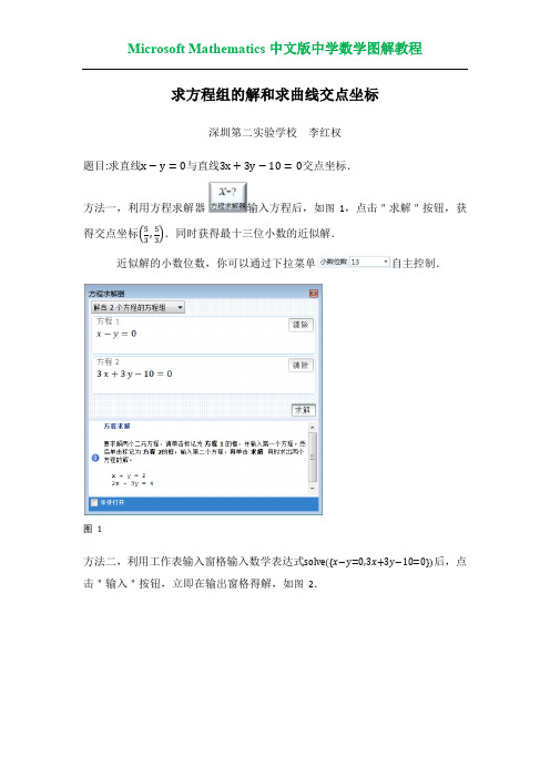
求方程组的解和求曲线交点坐标
深圳第二实验学校 题目:求直线 与直线 李红权 交点坐标.
方法一,利用方程求解器 得交点坐标
输入方程后,如图 1,点击"求解"按钮,获
.同时获得最十三位小数的近似解. 自主控制.
近似解的小数位数,你可以通过下拉菜单
图 1
方法二,利用工作表输入窗格输入数学表达式 击"输入"按钮,立即在输出窗格得解,如图 2.
后,点Leabharlann icrosoft Mathematics 中文版中学数学图解教程
图 2
特别提示:如图 3,同样是解方程组 与”nsolve”的区别.
,请注意”solve”
图 3
2018年秋新课堂高中数学人教A版选修1-2教师用书:第2章 2.2 2.2.1 综合法和分析法

2.2直接证明与间接证明2.2.1综合法和分析法学习目标:1.理解综合法、分析法的意义,掌握综合法、分析法的思维特点.(重点、易混点)2.会用综合法、分析法解决问题.(重点、难点)[自主预习·探新知]1.综合法思考1:综合法与分析法的推理过程是合情推理还是演绎推理?[提示]综合法与分析法的推理过程是演绎推理,因为综合法与分析法的每一步推理都是严密的逻辑推理,从而得到的每一个结论都是正确的,不同于合情推理中的“猜想”.思考2: 综合法与分析法有什么区别?[提示]综合法是从已知条件出发,逐步寻找的是必要条件,即由因导果;分析法是从待求结论出发,逐步寻找的是充分条件,即执果索因.[基础自测]1.思考辨析(1)综合法是执果索因的逆推证法.()(2)分析法就是从结论推向已知.()(3)所有证明的题目均可使用分析法证明.()[答案](1)×(2)×(3)×2.命题“对于任意角θ,cos4θ-sin4θ=cos 2θ”的证明:“cos4θ-sin4θ=(cos2θ-sin2θ)(cos2θ+sin2θ)=cos2θ-sin2θ=cos 2θ”,其过程应用了()【导学号:48662070】A.分析法B.综合法C.综合法、分析法综合使用D.间接证法B[从证明过程来看,是从已知条件入手,经过推导得出结论,符合综合法的证明思路.]3.要证明A>B,若用作差比较法,只要证明________.A-B>0[要证A>B,只要证A-B>0.]4.将下面用分析法证明a2+b22≥ab的步骤补充完整:要证a2+b22≥ab,只需证a2+b2≥2ab,也就是证________,即证________,由于________显然成立,因此原不等式成立.a2+b2-2ab≥0(a-b)2≥0(a-b)2≥0[用分析法证明a2+b22≥ab的步骤为:要证a2+b22≥ab成立,只需证a2+b2≥2ab,也就是证a2+b2-2ab≥0,即证(a-b)2≥0.由于(a-b)2≥0显然成立,所以原不等式成立.][合作探究·攻重难](1)已知a,b是正数,且a+b=1,证明:1a+1b≥4.(2)在△ABC中,a,b,c分别为内角A,B,C的对边,且2a sin A=(2b-c)sin B +(2c-b)sin C.①求证:A的大小为π3;②若sin B+sin C=3,证明△ABC为等边三角形.【导学号:48662071】[证明](1)法一:因为a,b是正数且a+b=1,所以a+b≥2ab,所以ab≤12,所以1a+1b=a+bab=1ab≥4.法二:因为a,b是正数,所以a+b≥2ab>0,1 a +1b≥21ab>0,所以(a+b)⎝⎛⎭⎪⎫1a+1b≥4.又a+b=1,所以1a +1b≥4.法三:1a+1b=a+ba+a+bb=1+ba+ab+1≥2+2ba·ab=4.当且仅当a=b时,取“=”号.(2)①由2a sin A=(2b-c)sin B+(2c-b)sin C,得2a2=(2b-c)b+(2c-b)c,即bc=b2+c2-a2,所以cos A=b2+c2-a22bc=12,所以A=π3.②因为A+B+C=180°,所以B+C=180°-60°=120°.由sin B+sin C=3,得sin B+sin( 120°-B)=3,sin B+(sin 120°cos B-cos 120°sin B)=3,32sin B+32cos B=3,即sin (B+30°)=1.因为0°<B<120°.所以30°<B+30°<150°,所以B+30°=90°,B=60°.所以A=B=C=60°,即△ABC为等边三角形.1.如图2-2-1所示,在四棱锥P-ABCD中,P A⊥底面ABCD,AB⊥AD,AC⊥CD,∠ABC=60°,P A=AB=BC,E是PC的中点.图2-2-1(1)证明:CD⊥AE;(2)证明:PD⊥平面ABE.[证明](1)在四棱锥P-ABCD中,∵P A⊥底面ABCD,CD⊂平面ABCD,∴P A⊥CD.∵AC⊥CD,P A∩AC=A,∴CD⊥平面P AC.而AE ⊂平面P AC ,∴CD ⊥AE .(2)由P A =AB =BC ,∠ABC =60°,可得AC =P A . ∵E 是PC 的中点,∴AE ⊥PC . 由(1)知,AE ⊥CD ,又PC ∩CD =C , ∴AE ⊥平面PCD .而PD ⊂平面PCD ,∴AE ⊥PD . ∵P A ⊥底面ABCD ,∴PD 在底面ABCD 内的射影是AD . 又AB ⊥AD ,∴AB ⊥PD .又∵AB ∩AE =A ,∴PD ⊥平面ABE .【导学号:48662072】[证明] 当a +b ≤0时,∵a 2+b 2≥0,∴a 2+b 2≥22(a +b )成立.当a +b >0时, 用分析法证明如下:要证a 2+b 2≥22(a +b ),只需证(a 2+b 2)2≥⎣⎢⎡⎦⎥⎤22(a +b )2.即证a 2+b 2≥12(a 2+b 2+2ab ),即证a 2+b 2≥2ab . ∵a 2+b 2≥2ab 对一切实数恒成立,∴a2+b2≥22(a+b)成立.综上所述,不等式得证.2.已知a,b是正实数,求证:ab+ba≥a+b.【导学号:48662073】[证明]要证ab+ba≥a+b,只要证a a+b b≥ab·(a+b).即证(a+b-ab)(a+b)≥ab(a+b),因为a,b是正实数,即证a+b-ab≥ab,也就是要证a+b≥2ab,即(a-b)2≥0.而该式显然成立,所以ab +ba≥a+b.[探究问题]1.在实际解题时,综合法与分析法是否可以结合起来使用?提示:在实际解题时,常常把分析法和综合法结合起来使用,即先利用分析法寻找解题思路,再利用综合法有条理地表述解答过程.2.你会用框图表示综合法与分析法交叉使用时的解题思路吗? 提示:用框图表示如下:其中P 表示已知条件、定义、定理、公理等,Q 表示要证明的结论.已知a 、b 、c 是不全相等的正数,且0<x <1. 求证:log x a +b 2+log x b +c 2+log x a +c2<log x a +log x b +log x c .思路探究:解答本题的关键是利用对数运算法则和对数函数性质转化成整式不等式证明.[证明] 要证明:log x a +b 2+log x b +c 2+log x a +c2<log x a +log x b +log x c , 只需要证明log x ⎝ ⎛⎭⎪⎫a +b 2·b +c 2·a +c 2<log x (abc ).由已知0<x <1,只需证明a +b 2·b +c 2·a +c2>abc . 由公式a +b 2≥ab >0,b +c 2≥bc >0,a +c2≥ac >0, 又∵a ,b ,c 是不全相等的正数,∴a+b2·b+c2·a+c2>a2b2c2=abc.即a+b2·b+c2·a+c2>abc成立.∴log x a+b2+log xb+c2+log xa+c2<log x a+log x b+log x c成立.1.欲证2-3<6-7成立,只需证()A.(2-3)2<(6-7)2B.(2-6)2<(3-7)2C.(2+7)2<(3+6)2D.(2-3-6)2<(-7)2C[∵2-3<0,6-7<0,故2-3<6-7⇔2+7<3+6⇔(2+7)2<(3+6)2.] 2. 在△ABC中,若sin A sin B<cos A cos B,则△ABC一定是()【导学号:48662074】A .直角三角形B .锐角三角形C .钝角三角形D .等边三角形C [由sin A sin B <cos A cos B 得cos(A +B )=-cos C >0,所以cos C <0,即△ABC 一定是钝角三角形.]3.如果a a +b b >a b +b a ,则实数a ,b 应满足的条件是________. a ≠b 且a ≥0,b ≥0 [a a +b b >a b +b a ⇔a a -a b >b a -b b ⇔a (a -b )>b (a -b ) ⇔(a -b )(a -b )>0⇔(a +b )(a -b )2>0, 只需a ≠b 且a ,b 都不小于零即可.]4.设a >0,b >0,c >0,若a +b +c =1,则1a +1b +1c 的最小值为________. 9 [因为a +b +c =1,且a >0,b >0,c >0,所以1a +1b +1c =a +b +c a +a +b +c b +a +b +c c =3+b a +a b +c b +b c +a c +c a ≥3+2b a ·ab +2c b ·bc +2c a ·ac =3+6=9.当且仅当a =b =c 时等号成立.]5.设a ≥b >0,求证:3a 3+2b 3≥3a 2b +2ab 2.(请用分析法和综合法两种方法证明)【导学号:48662075】[证明] 法一:3a 3+2b 3-(3a 2b +2ab 2)=3a 2(a -b )+2b 2(b -a )=(3a 2-2b 2)(a -b ).因为a ≥b >0,所以a -b ≥0,3a 2-2b 2>0,从而(3a 2-2b 2)(a -b )≥0, 所以3a 3+2b 3≥3a 2b +2ab 2.法二:要证3a 3+2b 3≥3a 2b +2ab 2,只需证3a 2(a -b )-2b 2(a -b )≥0,只需证(3a2-2b2)(a-b)≥0,∵a≥b>0.∴a-b≥0,3a2-2b2>2a2-2b2≥0,∴上式成立.。
2012感动二实人物事迹材料(10位)(2013-1-9)

2012年“感动‘二实’年度人物”候选人事迹材料1.校毽球队关键词:体坛明星,享誉世界清晨,人们还在睡梦中,他们早已开始了一小时的晨练;傍晚,无论严寒酷暑,他们始终坚持训练三小时;周六、周日,他们从不休息,进行从难、从严、从实战出发的适度极限训练;为了中华毽球的传承、弘扬和腾飞,他们甘吃苦中苦,愿求苦中“乐”;他们中先后有8人次获得世界冠军,140多人次获全国冠军……2012年他们发挥敢打敢拼的运动精神,以破竹之势在国内外的毽球赛场上,赛出了风格和水平:广东省第十届中学生运动会毽球赛包揽了全部14枚金牌,广东省毽球锦标赛获得5金6银6铜,全国毽球锦标赛获4金5银3铜,在法国举行的国际毽球公开赛喜获冠亚军。
他们不仅赢得了省内同行的一致赞誉,国家体育总局和毽协领导的首肯,在国际比赛中也给国际毽坛带来了巨大的震撼。
他们还曾两次远赴宁夏和新疆,进行“中国毽球西部行”活动,为毽球运动的推广作出了重大的贡献。
2.有效教学团队(高二、初二有效教学教师)关键词:改革先锋,教坛亮点有效教学团队是我校有效教学课堂模式改革的先锋队,它的成立凝聚了校长、专家、部门领导和高二、初二年级教师的心血。
高中19位、初中13位一线教学人员执行有效教学高效课堂行为坚定,不斤斤计较,不辞劳苦,不计报酬,不忧谗畏讥。
几个月以来,高初中有效教学团队对学生培训62场次,自身培训研究近60次,每周例会研讨课堂教学;这个团队人人都上公开课,本学期承担各类公开课、展示课、研究课、汇报课、录像课等多达120节;这个团队个个都在写教学文章,共计26篇,在校级课堂教研、学校评估、校际交流等方面发挥了巨大的作用。
“实验探索,初显端倪,成绩显著,成效喜人”这是专家对有效教学的阶段性评价。
有效教学的“高效课堂”已逐渐成为学校的一个亮点,学生已成为课堂学习的主体,并且积累了一定“有用”的资料,开发了大量的学习工具单,有效教学的行动还激发了老师们积极探索教改的热情。
2024年MATLAB基础教程(第五版)全套教学课件

35
优化工具箱使用方法
线性规划
使用MATLAB的优化工具箱可以方便地 求解线性规划问题,如最小二乘法、线
性约束优化等。
整数规划
2024/2/29
对于整数规划问题,优化工具箱提供 了分支定界法、割平面法等求解方法
。
非线性规划
优化工具箱也支持非线性规划问题的 求解,如梯度下降法、牛顿法等。
多目标优化
优化工具箱还支持多目标优化问题的 求解,如遗传算法、粒子群算法等。
MATLAB概述与基础
2024/2/29
4
MATLAB简介及应用领域
01
MATLAB是MathWorks公司 开发的一款商业数学软件
2024/2/29
02
主要应用于算法开发、数据 可视化、数据分析以算、工程设计、图 像处理、信号处理等领域有
广泛应用
5
MATLAB工作环境与界面介绍
36
信号处理工具箱应用实例
信号滤波
使用信号处理工具箱可 以对信号进行滤波处理 ,如低通、高通、带通
滤波等。
2024/2/29
频谱分析
信号处理工具箱提供了 丰富的频谱分析工具, 如傅里叶变换、功率谱
分析等。
波形生成与调制
可以生成各种标准波形 并进行调制处理,如正 弦波、方波、AM调制
等。
37
信号重构与压缩
和微积分等操作。
02
图形界面开发
MATLAB提供了丰富的图形界 面开发工具,可以方便地创建
交互式界面。
03
外部接口与编程
MATLAB支持与其他编程语言 的接口,如C/C、Java等,方
便进行混合编程。
04
并行计算
MATLAB支持并行计算,可以 利用多核处理器和计算机集群
陕西省石泉县高中数学第一章推理与证明1.2综合法和分析法1.2.2分析法二教案北师大版选修2_2

课标要求
结合已经学过的数学实例,了解直接证明的两种基本方法:分析法和综合法;了解分析法和综合法的思考过程、特点
三维目标
1.知识与技能
(1)引导学生分析综合法和分析法的思考过程与特点;
(2)简单运用综合法与分析法解决具体的数学问题.
2.过程与方法
结合学生已学过的数学知识,通过实例引导学生分析综合法与分析法的思考过程与特点,并归纳出操作流程.
所以 .
同理 .
这样就证明了△EHF为等腰三角形.
所以HG⊥EF.
例2:已知:a,b,c都是正实数,且ab+bc+ca=1.求证:a+b+c .
证明:考虑待证的结论“a+b+c ” ,因为a+b+c>0,
只需证明 ,
即 .
又ab+bc+ca=1,
所以,只需证明 ,
即 .
因为ab+bc+ca=1,
所以,只需证明 只需证明 ,
(二)、引入新课
分析法和综合法是思维方向相反的两种思考方法。在数学解题中,分析法是从数学题的待证结论或需求问题出发,一步一步地探索下去,最后达到题设的已知条件。综合法则是从数学题的已知条件出发,经过逐步的逻辑推理,最后达到待证结论或需求问题。对于解答证明来说,分析法表现为执果索因,综合法表现为由果导因,它们是寻求解题思路的两种基本思考方法,应用十分广泛。在很多数学命题的证明中,往往需要综合地运用这两种思维方法
3.情感、态度与价值观
(1)通过本节的学习,使学生在以后的学习和生活中,能自觉地、有意识地运用这些方法进行数学证明,养成言之有理、论证有据的习惯;
(2)通过本节的学习和运用实践,体会数学问题解决过程中的思维方式.
Summary

NASA Technical Memorandum4435 Hypersonic Lateral and Directional Stability Characteristics of Aeroassist Flight Experiment Configuration in Air and CF4John R.Micol and William L.WellsMAY1993NASA Technical Memorandum4435 Hypersonic Lateral and Directional Stability Characteristics of Aeroassist Flight Experiment Configuration in Air and CF4John R.Micol and William L.WellsLangley Research CenterHampton,VirginiaSummaryThe proposed Aeroassist Flight Experiment (AFE)utilized a14-ft-diameter raked and blunted elliptical cone to demonstrate the ight character-istics of space transfer vehicles(STV's).The AFE was to be carried to orbit by and launched from the Space Shuttle orbiter,where instrumentation for 10on-board experiments would have obtained aero-dynamic and aerothermodynamic data for velocities near32000ft/sec at altitudes above245000ft.A pre ight ground-based test program was initiated to assess the aerodynamic and aerothermodynamic characteristics of the baseline concept and to pro-vide benchmark data for calibration of computational uid dynamics codes to be used in ight predictions. The data reported herein are results from one phase of this ground-based study.Static lateral and di-rectional stability characteristics were obtained for the AFE con guration at angles of attack from010 to10 .Tests were conducted in air at Mach num-bers of6and10and in tetra uoromethane(CF4) at Mach6to examine the e ects of Mach number, Reynolds number,and normal-shock density ratio.Changes in Mach number from6to10in air or in Reynolds number by a factor of4at Mach6had a negligible e ect on the lateral and directional sta-bility characteristics of the baseline AFE con gura-tion.Variations in density ratio across the normal portion of the bow shock from approximately5(air) to12(CF4)had a measurable e ect on lateral and di-rectional aerodynamic coe cients,but no signi cant e ect on lateral and directional stability character-istics.The tests in air and CF4indicated that the con guration was laterally and directionally stable through the test range of angle of attack.Unfortunately,the AFE program was cancelled in late1991.The realization of an AFE ight in the future is possible but uncertain.Thus,this paper documents the lateral and directional aerodynamic characteristics of the baseline AFE vehicle for use in the design of future aeroassist space transfer vehicles. IntroductionAmong the space transportation systems pro-posed for the future are space transfer vehicles (STV's),which are designed to ferry cargo between higher Earth orbits(for example,geosynchronous and lunar orbits)and lower Earth orbit where the Space Shuttle and Space Station Freedom will op-erate.(This class of vehicle was formerly referred to as orbital transfer vehicles or OTV's.)Upon re-turn of the vehicle from high Earth orbit,its velocity must be greatly reduced to attain a nearly circular low Earth orbit.This decrease in velocity can be achieved either by using retrorockets or by guiding the vehicle through a portion of the atmosphere and allowing aerodynamic drag forces to slow the vehi-cle.Studies have shown that lower propellant loads would be required for the aeroassist method(ref.1); thus,payloads could be increased.Future STV's that will be designed to use Earth atmosphere for deceleration are generally referred to as aeroassisted space transfer vehicles or ASTV's (formerly AOTV's).These vehicles will have high drag and a relatively low lift-to-drag ratio and will y at very high altitudes and velocities throughout the atmospheric portion of the trajectory.Before the actual ight vehicle can be designed with optimal aerodynamic and aerothermodynamic characteris-tics,additional information about very high-altitude, high-velocity ight is required.To obtain such in-formation,a subscale ight was proposed whereby a14-ft-diameter ASTV con guration with10on-board experiments would be launched from the Space Shuttle and accelerated back into the atmosphere with a rocket.This Aeroassist Flight Experiment (AFE)would make a sweep through the atmosphere to an altitude of about245000ft with a velocity of nearly32000ft/sec to gain aerodynamic and aero-thermal information and return to low Earth orbit for retrieval by the Space Shuttle.The on-board in-strumentation would measure and record the aero-dynamic characteristics and aerothermodynamic en-vironment of this entry trajectory,and the data would be used to validate computational uid dy-namics(CFD)computer codes and ground-to- ight extrapolation of experimental data for use in future ASTV designs.This ight experiment was proposed because the high-velocity,low-density ow environ-ment cannot be duplicated or simulated in present test facilities,nor can it be predicted with certainty by existing techniques.Naturally,the AFE would require an extensive aerodynamic and aerothermodynamic experimental and computational data base for its design and suc-cessful ight.Present test facilities,in conjunction with the best CFD codes,would provide this infor-mation.For this reason,a pre ight test program in ground-based hypersonic facilities(ref.2)was initiated to develop the required aerodynamic and aerothermodynamic data base.This data base will be used to perform the rst phase of CFD computer code calibration.The experimental results presented herein are part of an extensive ground-based test program performed at the Langley Research Center. Previous results are presented in references3{6.The details of the rationale for the ight experiment areoutlined in reference7,and the set of experiments to be performed is described in reference8.A primary concern for the AFE vehicle is the aerothermal heating on the fore-and aftbody thermal protection system(TPS).Because of these aerother-mal concerns,low values of sideslip angles are desir-able to minimize heating to the aftbody or payload and to prevent large thermal uctuations on the heat shield.Thus,an accurate knowledge of the lateral and directional stability characteristics of the AFE is required.(Lateral and directional stability require-ments for a low lift-to-drag aeromaneuvering vehicle are discussed in ref.9.)CFD codes are not generally used to provide aero-dynamic information for vehicles at sideslip angles. Computed lateral and directional stability charac-teristics for the AFE would require calculations of the entire body at various sideslip angles,thus in-creasing computational time,complexity,and cost. Hence,determination of these stability characteris-tics for the ight vehicle must rely on experimental data obtained in ground-based facilities.This paper addresses the e ects of Mach number, Reynolds number,and normal-shock density ratio(a \real gas"simulation parameter)on lateral and direc-tional aerodynamic characteristics measured on the baseline AFE con guration.Tests were conducted at Mach6and10in air and at Mach6in tetra- uoromethane(CF4)through a range of angle of at-tack and sideslip.During the continuum- ow portion of the ight, the AFE vehicle is expected to undergo normal-shock density ratios of about18,whereas conventional hy-personic wind tunnels that use air or nitrogen as the test gas only produce ratios of5to7.In ight,this large density ratio results from dissociation of air as it passes into the high-temperature shock layer.This real-gas e ect may have a signi cant impact on shock detachment distance,distributions of heating and pressure,and aerodynamic characteristics(ref.10).For blunt bodies at hypersonic speeds,the pri-mary factor that governs the shock stand-o distance and inviscid forebody ow is the normal-shock den-sity ratio.(See ref.10.)Certain aspects of a real gas can be simulated by the selection of a test gas that has a low ratio of speci c heats and provides large values of density ratio.These conditions can be obtained in the Langley Hypersonic CF4Tun-nel,which provides a simulation of this phenomenon by producing a density ratio of about12across the shock.This tunnel,in conjunction with the Lang-ley20-Inch Mach6Tunnel,provides the capability to test a given model at the same free-stream Mach number and Reynolds number,but at two values of density ratio(5.25in air and12.0in CF4).Thus, data for code calibration are provided that include the e ects of normal-shock density ratio.Tests were performed in air at Mach10and through a range of Reynolds numbers at Mach6to verify that aerody-namic characteristics were independent of signi cant changes in Mach numbers and Reynolds numbers for the blunt AFE con guration in hypersonic contin-uum ow.However,the AFE program cancellation ended the research e orts on this con guration.Thus, this paper documents the lateral and directional characteristics of the baseline AFE vehicle for use in the design of future aeroassist space transfer vehicles. SymbolsC l rolling-moment coe cient,Rolling momentq1dSC l=1C l=1 ;per degC n yawing-moment coe cient,Yawing momentq1dSC n =1C n=1 ,per degC y side-force coe cient,Side forceq1SC y=1C y=1 ,per degd model length in symmetry plane,in.M Mach numberp pressure,psiaq dynamic pressure,psiaRe1unit free-stream Reynoldsnumber,ft01Re2;d postshock Reynolds numberbased on dS reference area,model base area,in2(10.604in2when d=3.67in.and4.936in2when d=2.50in.)T temperature, RU velocity,ft/secX moment transfer distance in axialdirection( g.4),in.(1.673in.when d=3.67in.and1.559in.when d=2.50in.)x;y;z axial,lateral,and vertical coordi-nates for AFE( g.4)2Z moment transfer distance innormal direction( g.4),in.(0.129in.when d=3.67in.and0.0979in.when d=2.50in.)angle of attack,degangle of sideslip,degratio of speci c heats of the testgasdensity of the test gas,lbm/in3 Subscripts:t total conditions1free-stream conditions2conditions behind the normalshockAFE Con gurationThe AFE ight vehicle would consist of a14-ft-diameter drag brake,an instrument carrier at the base,a solid-rocket propulsion motor,and small control motors.A sketch of the vehicle is shown in gure1.The drag brake( g.2),which is the forebody con guration,is derived from a blunted 60 half-angle elliptical cone that is raked at73 to the cone centerline to produce a circular raked plane.A skirt with an arc radius equal to one-tenth the rake-plane diameter and with an arc length corresponding to60 has been attached to the rake plane to reduce aerodynamic heating around the base periphery.The blunt nose is an ellipsoid with an ellipticity equal to2.0in the symmetry plane.The ellipsoid nose and the skirt are at a tangent at their respective intersections to the elliptical cone surface.A detailed description of the forebody analytical shape is presented in reference11.Apparatus and TestsFacilitiesLangley31-Inch Mach10Tunnel.The Langley31-Inch Mach10Tunnel(formerly the Lang-ley Continuous Flow Hypersonic Tunnel)expands dry air through a three-dimensional contoured nozzle to a31-in-square test section to achieve a nominal Mach number of10.The air is heated to approxi-mately1850 R by an electrical resistance heater,and the maximum reservoir pressure is approximately 1500psia.The tunnel operates in the blowdown mode with run times of approximately60sec.Force and moment data can be obtained through a range of angle of attack or sideslip during one run by uti-lization of the pitch-pause capability of the model support system.This tunnel is described in more detail in reference12.Langley20-Inch Mach6Tunnel.The20-Inch Mach6Tunnel is a blowdown wind tunnel that uses dry air as the test gas.The air may be heated to a maximum temperature of approximately1100 R by an electrical resistance heater;the maximum reser-voir pressure is525psia.A xed-geometry,two-dimensional,contoured nozzle with parallel side walls expands the ow to a Mach number of6at the20-in-square test section.The model injection mechanism allows changes in angle of attack and sideslip during a run.Run durations are usually60to120sec,al-though longer times can be attained by connection to auxiliary vacuum storage.A description of this facility and the calibration results are presented in reference13.Langley20-Inch Mach6CF4Tunnel.The 20-Inch Mach6CF4Tunnel is a blowdown wind tunnel that uses CF4as the test gas.The CF4 can be heated to a maximum temperature of1530 R by two molten lead bath heat exchangers connected in parallel.The maximum pressure in the tunnel reservoir is2600psia.Flow is expanded through an axisymmetric,contoured nozzle designed to generate a Mach number of6at the20-in-diameter exit.This facility has an open-jet test section.Run duration can be as long as30sec,but10sec is su cient for most tests because the model injection system is not presently capable of changing angle of attack or sideslip during a run.A detailed description of the20-Inch Mach6CF4tunnel is presented in reference14.Just before the present test series,the tunnel was modi ed extensively.Included in those modi cations were a new nozzle,a new test section and model in-jection system,a new di user,and improvements in wiring of the controls and of the data acquisition system.The new nozzle was designed to improve ow quality along the centerline and to more closely match the Mach number in the Mach6air tunnel that is often used to produce data for comparison with the CF4data.Calibration results(ref.15)that were obtained after the new nozzle was installed indi-cate greatly improved ow uniformity near the nozzle centerline.For the present test series,the model was tested on the tunnel centerline.Previously,models were tested o centerline to avoid ow disturbances. (See ref.14.)3ModelsTwo aerodynamic models were fabricated and tested.The models were identical except for size;the base heights(d in g.2)at the symmetry plane were 3.67in.(2.2percent scale)as shown in gure3(a)and 2.50in.(1.5percent scale)as shown in gure3(b). The3.67-in-diameter model is made in three parts| a stainless steel forebody(aerobrake),an aluminum aftbody(instrument carrier and propulsion motor), and a stainless steel balance holder.The2.50-in-diameter model,shown mounted in the Langley 20-Inch Mach6CF4Tunnel in gure3(c),is fabri-cated of aluminum and does not include the circu-lar or hexagonally shaped aftbody and the simulated propulsion motor of previous models that were tested (ref.16).A cylinder protrudes from the base to ac-cept the balance.The acute angle between the bal-ance and cylinder axis and the base in the symmetry plane is73 .The2.50-in-diameter model was fabri-cated to provide an air gap between the end of the balance and the end of the cavity in the forebody; its purpose was to reduce conductive heating.For both models,shrouds were built to shield the bal-ance from base- ow closure.The shrouds attach to the sting,and clearance was provided to avoid in-terference with the balance during model movement when forces and moments were applied.The fore-bodies were machined to the design size and shape within a tolerance of60.003in.Angle of attack(see g.2)and sideslip(see g.4)in this paper are refer-enced to the axis of the original elliptical cone.InstrumentationAerodynamic force and moment data were mea-sured with sting-supported,six-component,water-cooled,internal strain gauge balances.Two ther-mocouples were installed in the water jacket that surrounds the measuring elements to monitor inter-nal balance temperatures.The load rating for each component of the two balances(one for each model size)is presented in table I.The calibration accuracy is0.5percent of the maximum load rating for each component.Test ConditionsThe tests were conducted at nominal free-stream Mach numbers of6and10in air and at Mach6 in CF4.(Nominal test conditions are presented in table II.)The angles of attack for Mach6in air were 0 and65 with nominal sideslip angles of0 ,02 , and04 .Tests at Mach6in CF4were at angles of attack of0 ,65 ,and610 with nominal sideslip angles of0 ,62.5 ,and65 ;at Mach10(except for =02:5 ,where only a negative sweep was performed),the angles of attack were0 ,62.5 ,65 , and610 with nominal sideslip angles of0 ,62 ,and 64 .Test ProceduresBlunt models are conducive to heat conduction through the forebody face during a run,which gener-ally produces a gradual increase in temperature gra-dients along the balance even though the balance is water cooled.Because temperature gradients were not accounted for in the laboratory calibration of the balance,e orts were made to minimize these gradi-ents by limiting the test times.In the20-Inch Mach6 CF4Tunnel,the model was mounted at the desired angle of attack and sideslip before the run.After the test-stream ow was established,the model was in-jected to the test-stream centerline.Data were gath-ered for approximately5sec,then the model was re-tracted.In the air tunnels,the model was mounted at = =0 before the run.After test-stream ow was established,the model was injected to the stream centerline,then pitched to the next angle of attack(or sideslip angle)by the pitch-pause mech-anism.Data were taken while the model was sta-tionary at each position.The balance thermocouples were monitored during each run to assure that the temperature gradient within the balance remained within an acceptable limit.Typical run times for a set of and sweeps in the air facilities were about 15sec.Data Reduction and UncertaintyEach of the three test facilities has a dedicated stand-alone data system.Output signals from the balances were sampled and digitized by an analog-to-digital converter,then stored and processed by a computer.The analog signals were sampled at a rate of50per second in the Mach6CF4and Mach10air tunnels and at20per second in the Mach6air tunnel.A single value of data reported herein represents an average of values measured for 2sec in the Mach6CF4and Mach6air tunnels and for0.5sec in the Mach10air tunnel.Corrections were made for model tare weights at each angle of attack and for interactions between di erent elements of the balances.Corrections were not made for base pressures.Balance-related calculated uncertainties in the measured static aerodynamic coe cients are given in table III.These uncertainties are based on balance output signals related to forces and moments by a laboratory calibration that is accurate to60.5per-cent of the rated load for each component.(See ta-ble I.)For the AFE,the moment reference center is4located at the center of the rake plane.(See g.4.) Thus,moments reduced about the model rake-plane center and reported herein have greater uncertainties than those measured at the balance moment center. The yawing and rolling moments at the balance have an uncertainty of only60.5percent of the rated load, whereas the moment at the rake-plane center also in-cludes uncertainties associated with the forces in the transfer equation.The transfer equation isYawing moment RP=Yawing moment B0(X)(Side force)andRolling moment RP=Rolling moment B0(Z)(Side force)where the subscripts RP and B denote the rake-plane center and the balance moment center,respectively. The transfer distances X and Z are de ned in g-ure4.In coe cient form,the uncertainty1related to the balance calibration for the side force is1C y=6(0:005)(Force rating)q1SThe uncertainty for the yawing moment is1C n;B=6(0:005)(Moment rating)q1dSand an identical equation applies for the rolling mo-ment.These balance uncertainties are su cient for measurements at the balance moment center.How-ever,at the rake-plane center,the yawing-moment uncertainty is1C n;RP=62401C n;B12+1C y X!2350:5and the rolling-moment uncertainty is1C l;RP=62401C l;B12+1C y Zd!2350:5Note that all the terms include the free-stream dy-namic pressure in the denominator so that the un-certainties are less at test conditions where q1is large|that is,at a higher Reynolds number rather than at a lower Reynolds number.The uncertainty in dynamic pressure is63percent.The ow condi-tions for which the present uncertainties have been calculated are presented in table II.Results and DiscussionsThe aerodynamic data from the Mach10air tests are tabulated in table IV.The Mach6results are presented in tables V and VI for air and in table VII for CF4.The test Reynolds number and model diameter are indicated in each table title.The aerodynamic coe cients C y,C n,and C l are plotted for an angle-of-sideslip range at various an-gles of attack in each facility and presented in g-ures5{7for Mach10in air,Mach6in air,and Mach6 in CF4,respectively.Data obtained at Mach6in air( g.6)indicated no e ect of Reynolds number on measured lateral and directional coe cients for a factor-of-4increase in postshock Reynolds num-ber.(Similar trends with respect to Reynolds num-ber were also observed for AFE longitudinal aero-dynamic characteristics presented in ref.16in which a negligible e ect of Reynolds number was noted for Mach6and10in air and at Mach6in CF4.) Therefore,the assumption is made that the e ect of Reynolds number on measured lateral and direc-tional data at Mach10in air and Mach6in CF4 is also negligible.The data are amenable to linear curve ts as shown in gures5{7,for which the ordi-nate scale is quite sensitive.These curves would be expected to go through the origin because the model was symmetrical about the pitch plane.However,as observed in gures5{7,an o set exists.This o set may be attributed to model misalignment or to any small stray signal in the data system that could cause a constant data o set because of the very small val-ues being measured relative to the load range of the balance.For example,if a slight misalignment of the model in the roll direction were introduced during model setup or if the balance location within the model were slightly misaligned,thereby producing a small o set in the center of gravity location(that is,within a few thousandths of an inch)in the side plane(y di-rection in g.4),then the e ect of the large axial-force component on this small moment arm may pro-duce a continuous bias in the measured quantities. For instance,from reference16at = =0 , Re1=0:462106/ft,and Mach6in CF4,the axial-force coe cient is1.382.The yawing-moment coe -cient,from table VII for similar conditions,is0.004. In much the same way as the change in the cen-ter of pressure in longitudinal aerodynamics is lo-cated,forming the ratio of yawing-moment coe -cient to axial-force coe cient yields the moment arm in the y direction,which for this case is approxi-mately0.003in.and thus within acceptable fabri-cation tolerances.A second linear curve,parallel to the data-faired curve,is drawn through the origin in5each part of gures 5{7.Values from measurements and the curve through the origin of gures 5{7are presented in tables IV{e of the slopes of these parallel curves through the origin to represent the lateral and directional stability derivatives should be valid because the data curves are linear through the test sideslip range.The lateral and directional stability derivatives are presented in gure 8and table VIII through the range of angle of attack for which tests were per-formed in each facility.For all test conditions,the con guration was laterally and directionally stable,as indicated by the positive values of C n and nega-tive values of C l .A comparison of lateral and direc-tional stability derivatives obtained at Mach num-bers of 6and 10in air illustrates no signi cant e ect of Mach number on stability characteristics ;a comparison of these stability derivatives with those obtained at Mach 6in CF 4indicates a small but measurable e ect of normal-shock density ratio on lateral and directional stability characteristics.Al-though the numerical values for air and CF 4are not greatly di erent,the data trends in air and CF 4ap-pear to be opposite.(Similar trends were observed in the longitudinal aerodynamic characteristics dis-cussed in ref.16.)This trend is most obvious for C l ,wherein the small numerical values require an expanded scale on the graph.The wind tunnel re-sults in CF 4are believed to be a better simulation of ight data than those in air because the shock de-tachment distance for CF 4is closer to the distance predicted for the actual ight case.(For example,see refs.6and 16.)Concluding RemarksStatic lateral and directional stability character-istics were obtained for the Aeroassist Flight Exper-iment (AFE)con guration through a range of angle of attack from 010 to 10 .Tests were conducted on two di erent-sized models at Mach numbers of 6and 10in air and at a Mach number of 6in tetra- uoromethane (CF 4).The e ects of Mach number,Reynolds number,and normal-shock density ratio on lateral and directional stability characteristics were examined.Changes in Mach number from 6to 10in air or in Reynolds number by a factor of 4at Mach 6had a negligible e ect on the lateral and directional sta-bility characteristics of the baseline AFE con gura-tion.Variations in density ratio across the normal portion of the bow shock from approximately 5(air)to 12(CF 4)had a measurable e ect on lateral and directional aerodynamic coe cients,but no signi -cant e ect on lateral and directional stability char-acteristics.The tests in air and CF 4indicated that the con guration is laterally and directionally stable through the test range of angle of attack as indicated by the positive values of C n and negative values of C l (positive e ective dihedral).In late 1991,the AFE program was cancelled and thus ended research e orts on this con guration.The realization of an AFE ight in the future is possible but uncertain.Hence,this paper documents the lateral and directional aerodynamic characteristics of the baseline AFE vehicle for use in the design of future aeroassist space transfer vehicles.NASA Langley Research Center Hampton,VA 23681-0001March 25,1993References1.Walberg,Gerald D.:A Review of Aeroassisted Orbit Transfer.AIAA-82-1378,Aug.1982.2.Wells,William L.:Wind-Tunnel Pre ight Test Program for Aeroassist Flight Experiment.Technical Papers|AIAA Atmospheric Flight Mechanics Conference ,Aug.1987,pp.151{163.(Available as AIAA-87-2367.)3.Wells,William L.:Free-Shear-Layer Turning Angle in Wake of Aeroassist Flight Experiment (AFE)Vehicle at Incidence in M =10Air and M =6CF4.NASA TM-100479,1988.4.Micol,John R.:Experimentaland Predicted Pressure and Heating Distributions for Aeroassist Flight Experiment Vehicle.J.Thermophys.&Heat Transf.,July{Sept.1991,pp.301{307.5.Wells,WilliamL.:SurfaceFlow and HeatingDistributions on a Cylinder in Near Wake of Aeroassist Flight Experi-ment (AFE)Con guration at Incidence in Mach 10Air.NASA TP-2954,1990.6.Micol,John R.:Simulation of Real-Gas E ects on Pres-sure Distributions for Aeroassist Flight Experiment Vehi-cle and Comparison With Prediction.NASA TP-3157,1992.7.Jones,Jim J.:The Rationale for an Aeroassist Flight Experiment.AIAA-87-1508,June 1987.8.Walberg,G.D.;Siemers,P.M.,III;Calloway,R.L.;and Jones,J.J.:The Aeroassist Flight Experiment.IAF Paper 87-197,Oct.1987.9.Gamble,Joe D.;Spratlin,Kenneth M.;and Skalecki,Lisa M.:Lateral Directional Requirements for a Low L/D Aeromaneuvering Orbital Transfer Vehicle.A Collection of Technical Papers|AIAA Atmospheric Flight Mechan-ics Conference,Aug.1984,pp.402{413.(Available as AIAA-84-2123.)610.Jones,Robert A.;and Hunt,James L.(appendix Aby James L.Hunt,Kathryn A.Smith,and Robert B.Reynolds and appendix B by James L.Hunt and Lillian R.Boney):Use of Tetra uoromethane To Simulate Real-Gas E ects on the Hypersonic Aero dynamics of Blunt Vehicles.NASA TR R-312,1969.11.Cheatwood,F.McNeil;DeJarnette,Fred R.;and Hamil-ton,H.Harris,II:Geometrical Description for a Pro-posed AeroassistedFlight ExperimentVehicle.NASA TM-87714,1986.ler, C.G.:Langley Hypersonic Aerodynamic/Aerothermodynamic Testing Capabilities|Present and Future.AIAA-90-1376,ler,Charles G.,III;and Gno o,Peter A.:PressureDistributions and Shock Shapes for12.84 /7 On-Axis and Bent-Nose Biconics in Air at Mach6.NASA TM-83222,1981.14.Midden,Raymond E.;and Miller,Charles G.,III:De-scription and Calibration of the Langley Hypersonic CF4 Tunnel|A Facility for Simulating Low Flow as Occurs for a Real Gas.NASA TP-2384,1985.15.Micol,John R.;Midden,Raymond E.;and Miller,CharlesG.,III:Langley20-Inch Hypersonic CF4Tunnel:A Facil-ity for Simulating Real-Gas E ects.AIAA-92-3939,July 1992.16.Wells,William L.:Measured and Predicted AerodynamicCoe cients and Shock Shapes for AeroassistFlight Exper-iment(AFE)Con guration.NASA TP-2956,1990.7。
高中数学PPT课件-综合法和分析法

此时,如果能把角和边统一起来,那么就可以进一步寻找角和边之间的关系,进而判断三角形 的形状,余弦定理正好满足要求.于是,可以用余弦定理为工具进行证明.
新知探究
证明:由A,B,C成等差数列,有 2B=A+C. ①
因为A,B,C为△ABC的内角,所以 A+B+C=180°. ②
新知探究
请对综合法与分析法进行比较,说出它们各自的特点.回顾以往的数学学习,说说你对这两种证 明方法的新认识.
综合法就是利用已知条件和某些数学定义、公理、定理等,经过一系列的推理论证,最后推导出所 要证明的结论成立. 分析法最大的特点就是执果索因. 注意
事实上,在解决问题时,我们把综合法和分析法结合起来使用:根据条件的结构特点去转化结
新知探究
知识要点 一般地,利用已知条件和某些数学定义、公理、定理等,经过一系列的推理论证,最后推导出所要 证明的结论成立,这种证明方法叫做综合法.其特点是“由因导果”.
新知探究
你能用框图 表示综合法
吗?
用P表示已知条件、已有的定义、 公理、定理等,Q表示所要证明的 结论.
则综合法可用框图表示如下:
于是尝试转化结论:统一函数名称,即把正切函数化为正(余)弦函数.把结论
转化为
cos2α
-
sin2α
=
1 2
(cos2β
-
sin2β)
再与
4sin2α - 2sin2β = 1 比较,发现只要把
cos2α - sin2α = 1 (cos2β - sin2β)的角的余弦转化为正弦,就能达到目的.
2
新知探究
=
1
-
DX11软件教程两水平因子分析Two-Level Factorial(第5课)中文版共38页

两水平因子分析介绍本教程演示如何将Design Expert®软件用于两水平因子分析设计。
这些设计将帮助您筛选许多因子,以发现至关重要的少数,也包括他们可能存在的交互作用。
如果你赶时间,跳过“Note备注,笔记”这一部分,这种侧边栏,是提供给那些想花更多的时间来探索事物的人的。
备注程序的基本特性:在继续学习本教程之前,请返回到一个通用的单因子实验教程。
此处将不详细介绍演示的功能。
你现在要分析的数据来自道格拉斯·蒙哥马利的教科书《实验的设计与分析》,约翰·威利和儿子公司,纽约出版社。
本案例:华夫板(晶圆薄片)制造商必须立即降低用于现场过滤器加工助剂的甲醛浓度,否则将被监管官员关闭(安全法规强制要求)。
为了系统地探索他们的操作方法,工艺工程师对关键因子进行了全因子两水平设计,包括当前水平的浓度和可接受的低浓度。
全因子设计实例的因子和水平在这些过程的每一次组合中,实验者都记录下过滤速率。
我们的目标是最大限度地提高滤液过滤速率,并尝试找到条件,允许减少甲醛浓度,即因子C。
这个案例研究展示了设计专家提供的,许多两水平设计的特点。
这会让你在成为一名强大用户的道路上走得很好。
让我们继续!备注如果温度等因子很难改变,该怎么办:理想情况下,实验的运行顺序将完全随机化,这是设计专家默认的实验安排。
如果由于一个或多个因子很难被快速改变,而无法实现这一点,请选择裂区设计。
但是,请记住,对于随机性中受到限制的因子,您将付出降低效率标准的代价。
在开始一个裂区之前,参加“特性之旅”,了解设计专家是如何设计这样一个实验的,以及在选择效应时要注意什么,等等。
设计实验启动程序并单击“新建设计”。
你现在看到屏幕上有四个分支项。
继续使用因子Factorial因子选项,这是默认的。
您将使用默认的选择: Randomized Regular Two Factorial常规随机化两水平因子分析(析因)。
两水平析因设计生成器备注Design Expert的Design builder设计建模,提供2到21个因子的完整和部分两水平因子设计,以2的幂(4、8、16…)表示,最多可运行512次(实验组合)。
- 1、下载文档前请自行甄别文档内容的完整性,平台不提供额外的编辑、内容补充、找答案等附加服务。
- 2、"仅部分预览"的文档,不可在线预览部分如存在完整性等问题,可反馈申请退款(可完整预览的文档不适用该条件!)。
- 3、如文档侵犯您的权益,请联系客服反馈,我们会尽快为您处理(人工客服工作时间:9:00-18:30)。
选择要擦除图像的函数解析式,单击 OK 按钮。如果需要清除全部图像,单击菜单 File 下的 New。
-3-
2.4 定义在闭区间上的函数 想画出定义在闭区间 [-1,3] 上 的 函 数 y=x2-2x-3 图 像 , 就 这 样 输 入 :
利用这个方法,您可以是顺利绘出分段函数的图像。但不能绘制含有 开端点的区间函数,除非其自然定义域是开区间。 注:-1 和 3 之间必须用分号隔开 2.5 图像窗口范围 如果您想让您的图像更舒适、 更美观地呈现在图像窗口中, 您可以改变窗口的显示范围 的数值,如图五,可以设置窗口的 x 轴和 y 轴上的最大值和最小值以及轴上标数的步长。
图十二
四. 怎样计算积分
用 Equation Grapher 能为您计算积分的值。 如图十三, 首先把函数模式改变为积分模式 。
图十三 然后,输入将要完成积分的函数解析式,即输入被积式,同时将积分上下界输入,并用
-7-
分号隔开。例如,我们要计算下面的这个积分式:
1 ( x )dx x 1
如图十四种这样输入:x+1/x; 1; 3(注:被积式、积分上限、积分下限均用分号隔开) 就像您看见的那样,积分区被填上了蓝色,并且,定积分的值会在记录面板中自动显示 出来。这样既有直观的图形,又有精确的数据。我们不得不感谢伟大的计算机发明者们和那 些软件工程师。
3
图十四
五. 怎样把图像用到其它程序中
用 Equation Grapher,可以非常方便的把图像复制粘贴到您的文字处理程序中,或者图 像编辑程序中。现在就跟着下面步骤练习: 1、 打开 Equation Grapher,画出函数图像。 2、 从编辑菜单选复制。如图十五
图十五
-8-
3、 打开您的文字处理程序,或图像处理程序,在菜单中选“编辑/粘贴”。 提示:如果您在贴图像后,再改变图像尺寸,有些程序做不到。这样就只好在 Equation Grapher 窗口中,调整图像大小到合适,重复步骤 2、3,得到满意的图像或 优秀打印效果为止。
六. 其它菜单键钮的功能
6.1 其它 菜单 下一级是一个数值列表菜单(如图十六)
图十六
图十七 在单击就可得到一个,如图十七那样,在您输入解析式或相关数值之前是一张空表。如 果您在相应的位置上输入解析式、自变量 x 的最大值和最小值,以及步长,按下运算“计算” 按钮, 就可以得到相应的函数及一个导数值列表。 按下 “复制到剪贴板”按钮复制到剪贴板 , 可以把该表复制到剪贴板上。 6.2 选项 菜单 语言选择 经过夜以继日的努力笔者完成了汉化工作, 现在无论你选择 English 或 Swedish
深圳碧波中学李红权
编写
2004 年 5 月第一稿 2006 年 10 月修订稿
- 11 -
三. 怎样分析函数
一旦您画出了函数图像,Equation Grapher 可以按您的要求自动地在图像上找出函数值 为零时的根、极大值或极小值,以及其它函数图像的交点等,如图十。
-5-
图十 图中标明的按钮功能依次如下: ------------- 求根,即函数值 y 为零时, 自变量 x 的值 ------------- 极大值 ------------- 极小值 -------------- 与 Y 轴的交点,求函数图在 Y 轴上的截距 -------------- 求交点,求两个函数的交点坐标 -------------- 已知 x 值计算相应的 y 值,即代数式求值 ------------- 已知 y 值计算相应的 x 值,即解方程 -------------- “曲线跟踪”按钮,它可以使一个红色小方框套在指定的函数图像上, 跟踪函数曲线的走势,同时也方便讲解,是观察或解说时最常用的按钮。用左键拖动红色小 方框套在曲线上缓缓移动,窗口的左下角就显示出鼠标指针所在的每一个点的纵横坐标。
图二十一 几乎跟所有的软件一样,有帮助目录、购买方法、上网联系等等。 需要特别说明的是,这里的帮助文件和笔者以前编译的《Equation Grapher 教程》是本
- 10 -
《Equation Grapher 简体中文版教程》的重要参考资料。 《Equation Grapher 简体中文版教程》 的作者之本意是,通过本教程使您在享受数学和 Equation Grapher 的时候,及时向 Equation Grapher 的版权所有者购买使用。本中文教程作者反对任何形式的 DB 行为!
图八 “放大”按钮 和“缩小”按钮 两个按钮可以只把您需要的那部分图像充分的显
示出来。这些功能就像任何的图形软件里的放大、缩小的一样。 用“放大选区”按钮 ,您可给在图像窗口中,
通过鼠标拖出一个长方形选区, 并立即被放大充满图像 窗口。如果您想恢复改变前的情形,那么“撤销放缩” 按钮 能把图像范围数值恢复到最近一次放缩改变
图十一 例如,求 y=x^2-3x-1 的最小值,画出函数图像,选中菜单栏的“求解/极小值”(单击工
-6-
具栏“极小值”按钮,效果相同) Equation Grapher 现在需要您用鼠标画一个范围。要达到这个目的,您需要移动鼠标箭 头到图像窗口内。 将箭头指到将要画出的矩形范围的左上角, 按下鼠标左键, 并且拖动鼠标 , 直到箭头到右下角为止,松开鼠标左键。这样您在图像上用鼠标滑出一个矩形范围(如图十 一) 。 如果在您选取的矩形范围内有多个函数图像,您还需在一个弹出的“选择函数”对话框 中确定您要的函数。如果您所选择的函数在指定区域内,存在极小值的话,那么它就会被 一个红色的小圆圈圈住。 所有的精确值都将出现在记录面板中, 您可以查找到极值点的坐标的精确值。 您所要分 析的其它精确数据,都可以在记录面板中找到(如图十二) 。特别说明,记录面板默认情况 下,是躲在坐标面板下面的,要察看到记录面板需挪动坐标面板。
Equation Grapher 简体中文版教程
李红权编写
一. 二. 三. 四. 五. 六. 七.
介绍 怎样绘制函数图像 怎样分析函数 怎样计算积分 怎样把图像用到其它程序中 其它菜单按钮功能 更多资讯
图一
-1-
一. 介绍
Equation Grapher 简体中文版,是深圳数学教师李红权利用业余时间,由 Equation Grapher3.2 完成汉化的,版权为 MF Soft International 所有,原先只有英文版和瑞典文版。 这是一款函数绘图与分析的软件, 可以说是最好的图形计算器, 满足一切数学或科学计算的 需要, 绘制好函数图像后还可以通过打印机输出或保存为位图! 也是数学教师不可多得的好 帮手。软件界面儒雅经典,操作轻松便捷,易学易懂。 Equation Grapher 简体中文版它能使您绘制, 像 y=2x 和 y=sin(x+10)-cos3x 这样的函数图 像(图一) 。在同一坐标系内它最多允许绘制 12 个函数图像,并用不同的颜色呈现出来(事 实上第 12 个已经不能再画出来了,应该说把坐标系算上才够 12 个 ) 。 在您已经绘出的函数图像上,Equation Grapher 简体中文版会按照您的要求自动找出所 绘图像函数的根、极大值、极小值、交点坐标等等。另外,它还能计算查看定积分区域和定 积分值。 您可以利用放大或缩小改变图像呈现的范围, 或者直接键入指定的数值范围。 如果您愿 意,您可以复制窗口中的图像,并粘贴到您的文字或图形处理程序(如 MS Word \ACDSee \Photoshop)中去。当然,您也可以把您正在做的工作保存起来,有时间接着再做。
二. 怎样绘制函数图像
2.1 输入函数解析式到解析式栏 把鼠标指针移到函数解析式的位置,输入函数解析式如图二那样:
图二 您可以通过电脑键盘输入解函数解析式,也可以通过 Equation Grapher 的函数面板(如 图三)用鼠标输入函数解析式。如果您是初次接触 Equation Grapher,可能您会更乐意使用 函数面板。
七. 更多资迅
如果您愿意让您的任何希望或对问题的建议进入将来的版本,请给 info@ 发送电子邮件。也可访问 /919.htm 以获得更多资讯。 (当然需要您有 较好的英文水平) 欢迎您对本教程的任何建议和意见,发送 Email 至 HQ529@ 或电话: 13249895580. 2 图像窗口 正确输入函数解析式后,然后按回车键 Enter,或者点击函数面板中的绿色的“EXE” 按钮,您所要的任何函数图像就出现在窗口中了,如图四,神奇吧?
图四
2.3 添加或擦掉函数 如果您想在同一窗口中,还要绘制更多函数图像,那就只需要重复上面的步骤。同一个 窗口最多可以绘制出 12 个图像,并且每个图像的颜色各不相同。想要把画出的图像擦掉, 只需单击工具栏上的那红色橡皮“擦除函数”按钮 ,从自动弹出的函数解析式列表中,
前的模样。 7 绘图支持的函数 2.7 2. 除了加、减、乘、除四个标准算术运算之外,左边 图九列出运算符号和函数都能被写入函数表达式。 您不 妨一一尝试各种函数的功能。 在您对 Equation Grapher 比较熟悉的时候,也许您 会觉得从菜单中挑选函数表达式, 还不如从键盘输入这 些函数更便捷。 一点解释: Sqrt 即“求平方根”。遗憾的是,平方根符号没有 出现在ANSI(美国国家标准化组织)符号列表中。 图九
都将方便地进入中文界面。 其余选项,我再作解释就是轻视您的智慧了,劳驾自己看图十八好了。
-9-
图十九
6.3 窗口 菜单 图十八 如图十九 6.4 Regression 图二十 Analyzer 回归分析器 菜单 回归分析器菜单,如图二十,Start 可以方便的调用回归分析器,而 Information 则会显 示关于回归分析器的信息。另外, Regression Analyzer 因为使用频率不高,所以不没有对 其进行汉化。 6.5 帮助 菜单
图五
图六
如果我们想更好地表现出三角函数图像,像 y=tanx 我们可以借助于,Equation Grapher 提供的三角函数范围按钮。如图六,先按三角函数按钮 图像如图七。 ,在按下执行按钮 。得到的