Abaqus(FAQ)-剑桥大学工程系网站
ABAQUS应用培训-01 ABAQUS软件简介
11 更方便和灵活的二次开发工具。ABAQUS基于高级语言的用户子程序为用 户开发自己的单元、材料和分析流程提供了强大的工具这也是广大非 线性高端用户选择ABAQUS并应用它进行了大量深入的研究工作的原因。 12 材料的剥离与失效可以在ABAQUS中得到很好的模拟包括模拟冲击材料 的双面磨损功能。另外ABAQUS的自适应网格功能为克服和补偿切割过程 的大变形带来的网格奇异造成的计算误差提供了有力的手段。 13 ABAQUS提供的多体动力学分析功能为机械设备的操纵和传动系统等机构 分析和运动过程模拟等提供了强有力的工具。
m
mm
in
Force
N
N
1bf
Mass
kg
பைடு நூலகம்
T (103kg) s
1bf s2/in
Time
s
s
Stress
Pa
MPa mJ (10-3J) t/mm3 mm/s2
psi
Energy Density Ace
J Kg/m3 m/s2
in 1bf 1bf s2/in4
18
2015/7/5
9
INP文件
⑥ ⑦ ⑧ ⑨
8
2015/7/5
4
ABAQUS软件的主要功能特点
2)求解器性能
⑩ ABAQUS具有强大的热固耦合分析功能。ABAQUS包括51种纯热传导和热电 耦合单元83种隐式和显式完全热固耦合单元覆盖杆、壳、平面应变、 平面应力、轴对称和实体各种单元类型包括一阶和二阶单元为用户 建模提供极大的方便。
7
2015/7/5
ABAQUS软件的主要功能特点
2)求解器性能
⑤ 材料非线性是ABAQUS非线性分析的一种重要类型。它具有丰富的材料模 型库,涵盖了弹性,包括超弹性和亚弹性、金属塑性、粘塑性、蠕变、 各向异性等各种材料特性。 在复合材料方面,ABAQUS允许多种方法定义复合材料单元。包括复合材 料壳单元、复合材料实体单元以及叠层实体壳单元。 方便用户进行灵活的建模和后处理。 ABAQUS提供了壳单元到实体单元的子模型功能和壳单元到实体单元的tie 约束功能,可以对复合材料局部重要区域方便地进行细节建模 用户自定义材料机械性能 (UMAT)子程序可以由用户定义各种复杂的机械 本构模型并使用在ABAQUS分析中,UMATs已经被广泛用于研究金属基体复 合材料, 固化, 纤维抽拔, 和其他对复合材料很重要的局部效应。
(完整版)Abaqus帮助文档整理汇总,推荐文档
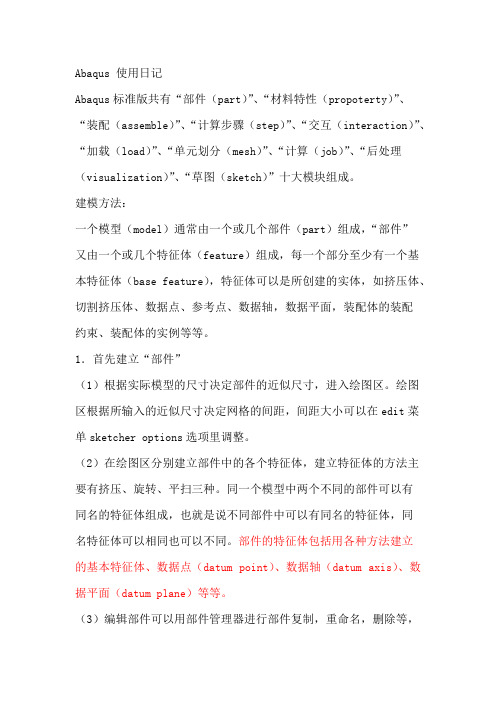
Abaqus 使用日记Abaqus标准版共有“部件(part)”、“材料特性(propoterty)”、“装配(assemble)”、“计算步骤(step)”、“交互(interaction)”、“加载(load)”、“单元划分(mesh)”、“计算(job)”、“后处理(visualization)”、“草图(sketch)”十大模块组成。
建模方法:一个模型(model)通常由一个或几个部件(part)组成,“部件”又由一个或几个特征体(feature)组成,每一个部分至少有一个基本特征体(base feature),特征体可以是所创建的实体,如挤压体、切割挤压体、数据点、参考点、数据轴,数据平面,装配体的装配约束、装配体的实例等等。
1.首先建立“部件”(1)根据实际模型的尺寸决定部件的近似尺寸,进入绘图区。
绘图区根据所输入的近似尺寸决定网格的间距,间距大小可以在edit菜单sketcher options选项里调整。
(2)在绘图区分别建立部件中的各个特征体,建立特征体的方法主要有挤压、旋转、平扫三种。
同一个模型中两个不同的部件可以有同名的特征体组成,也就是说不同部件中可以有同名的特征体,同名特征体可以相同也可以不同。
部件的特征体包括用各种方法建立的基本特征体、数据点(datum point)、数据轴(datum axis)、数据平面(datum plane)等等。
(3)编辑部件可以用部件管理器进行部件复制,重命名,删除等,部件中的特征体可以是直接建立的特征体,还可以间接手段建立,如首先建立一个数据点特征体,通过数据点建立数据轴特征体,然后建立数据平面特征体,再由此基础上建立某一特征体,最先建立的数据点特征体就是父特征体,依次往下分别为子特征体,删除或隐藏父特征体其下级所有子特征体都将被删除或隐藏。
××××特征体被删除后将不能够恢复,一个部件如果只包含一个特征体,删除特征体时部件也同时被删除×××××2.建立材料特性(1)输入材料特性参数弹性模量、泊松比等(2)建立截面(section)特性,如均质的、各项同性、平面应力平面应变等等,截面特性管理器依赖于材料参数管理器(3)分配截面特性给各特征体,把截面特性分配给部件的某一区域就表示该区域已经和该截面特性相关联3.建立刚体(1)部件包括可变形体、不连续介质刚体和分析刚体三种类型,在创建部件时需要指定部件的类型,一旦建立后就不能更改其类型。
ABAQUS关键字(keywords)

ABAQUS关键字(keywords)ABAQUS帮助里关键字(keywords)翻译(2013-03-06 10:42:48)转载▼分类:abaqus转自人人网总规则1、关键字必须以*号开头,且关键字前无空格2、**为注释行,它可以出现在中的任何地方3、当关键字后带有时,关键词后必须采用逗号隔开4、参数间都采用逗号隔开5、关键词可以采用简写的方式,只要程序能识别就可以了6、不需使用隔行符,如果参数比较多,一行放不下,可以另起一行,只要在上一行的末尾加逗号便可以----------------------------------------------------------------------------------------------------------------------------------------- *AMPLITUDE:幅值这个选项允许任意的载荷、和其它指定的数值在一个分析步中随时间的变化(或者在ABAQUS/Standard分析中随着的变化)。
必需的参数:NAME:幅值曲线的名字可选参数:DEFINITION:设置definition=Tabular(默认)给出表格形式的幅值-时间(或幅值-频率)定义。
设置DEFINITION=EQUALLY SPACED/PERIODIC/MODULATED/DECAY/SMOOTHSTEP/SOLUTION DEPENDENT或BUBBLE来定义其他形式的幅值曲线。
INPUT:设置该参数等于替换输入文件名字。
TIME:设置TIME=STEP TIME(默认)则表示分析步时间或频率。
TIME=TOTAL TIME表示总时间。
VALUE:设置VALUE=RELATIVE(默认),定义相对幅值。
VALUE=ABSOLUTE表示绝对幅值,此时,行中载荷选项内的值将被省略,而且当温度是指定给已定义了温度TEMPERATURE=GRADIENTS(默认)梁上或壳上的,不能使用ABSOLUTE。
ABAQUS功能简介

最先进的大型通用非线性有限元分析软件——ABAQUS1、概述美国ABAQUS软件公司成立于1978年,总部位于美国罗德岛博塔市,专门从事非线性有限元力学分析软件ABAQUS的开发与维护。
公司总部雇员400余人,其中近130余人具有工程或计算机博士学位,近120人具有硕士学位,被公认为世界上最大且最优秀的固体力学研究团体。
ABAQUS公司不断吸取最新的分析理论和计算机技术,领导着全世界非线性有限元技术的发展。
ABAQUS是国际著名的CAE软件,它以其强大的非线性分析功能以及解决复杂和深入的科学问题的能力赢得广泛称誉。
ABAQUS软件已被全球工业界广泛接受,并拥有世界最大的非线性力学用户群。
ABAQUS已成为国际上最先进的大型通用非线性有限元分析软件。
ABAQUS软件,除普通工业用户外,也在以高等院校、科研院所等为代表的高端用户中得到广泛。
研究水平的提高引发了用户对高水平分析工具需求的加强,作为满足这种高端需求的有力工具,ABAQUS软件在各行业用户群中所占据的地位也越来越突出。
ABAQUS是一个推崇技术的公司,它始终走在结构力学研究和软件化领域的前沿,它良好的品质和服务得到业界的广泛认可。
制造业是ABAQUS最重要的应用领域之一,拥有NASA、罗克希德-马丁、波音、空中客车等长期合作的用户。
对制造业很多复杂和特殊的问题,如热传导、爆炸冲击、流固耦合、疲劳断裂、复合材料损伤、接触连接、金属塑性等,在所有的CAE软件中,ABAQUS是最有优势的。
目前ABAQUS软件在中国的用户已超过800家,涵盖汽车、航空航天、船舶、武器、工程机械、建筑、电子、石化和核能源等各个领域,如宝山钢铁集团、长春一汽、上海泛亚、中国船级社、北京石化设计院、江钻股份、摩托罗拉和诺基亚等。
2、功能介绍ABAQUS软件的功能可以归纳为线性分析、非线性分析和机构分析三大块。
•线性静力学、动力学和热传导–静强度/刚度、动力学和模态、热力学和声学等–金属和复合材料、应力、振动、 声场、压电效应等•非线性和瞬态分析–汽车碰撞、飞机坠毁、电子器件跌落, 冲击和损毁等–复合材料损伤、接触, 塑性失效, 断裂和磨损, 橡胶超弹性等 •多体动力学分析–起落架收放、副翼展开、汽车悬架、微机电系统MEMS、医疗器械等–结合刚体和柔体模拟各种连接件,进行运动过程的力学分析3、模块介绍ABAQUS软件主要由ABAQUS/CAE,ABAQUS/Standard,ABAQUS/Explicit三个模块组成。
ABAQUS基础PPT课件

School of Transportation, Southeast University
.
14
ABAQUS约定1:单位
Quantity SI
SI (mm) US Unit (ft) US Unit (inch)
Length
m
mm
ft
in
Force
N
N
lbf
lbf
Mass
kg tonne (103 kg) slug
➢ ⑧格式(option=value)可用格式(-option value)代替。
School of Transportation, Southeast University
.
19
4 ABAQUS中的常用命令
➢用于获取信息的命令(Execution procedure for obtaining information)
➢ abaqus {help | information={environment | local | memory | release | status | support | system | all} [job=job-name] | whereami}
最常用命令:abaqus help(用来获取ABAQUS 所有命令)
和命令行接口 (Command line interface)
School of Transportation, Southeast University
.
7
2.2 ABAQUS/CAE中的分析模块(Modules)
➢ 分析模块
➢ 部件(Part) ➢ 特性(Property) ➢ 装配(Assembly) ➢ 分析步(Step) ➢ 相互作用(Interaction) ➢ 载荷(Load) ➢ 网格(Mesh) ➢ 作业(Job) ➢ 可视化(Visualization) ➢ 草图(Sketch)
ABAQUS入门手册

ABAQUS入门使用手册一、前言ABAQUS是国际上最先进的大型通用有限元计算分析软件之一,具有惊人的广泛的模拟能力.它拥有大量不同种类的单元模型、材料模型、分析过程等。
可以进行结构的静态与动态分析,如:应力、变形、振动、冲击、热传递与对流、质量扩散、声波、力电耦合分析等;它具有丰富的单元模型,如杆、梁、钢架、板壳、实体、无限体元等;可以模拟广泛的材料性能,如金属、橡胶、聚合物、复合材料、塑料、钢筋混凝土、弹性泡沫,岩石与土壤等.对于多部件问题,可以通过对每个部件定义合适的材料模型,然后将它们组合成几何构形。
对于大多数模拟,包括高度非线性问题,用户仅需要提供结构的几何形状、材料性能、边界条件、荷载工况等工程数据。
在非线性分析中,ABAQUS能自动选择合适的荷载增量和收敛准则,它不仅能自动选择这些参数的值,而且在分析过程中也能不断调整这些参数值,以确保获得精确的解答。
用户几乎不必去定义任何参数就能控制问题的数值求解过程.1.1 ABAQUS产品ABAQUS由两个主要的分析模块组成,ABAQUS/Standard和ABAQUS/Explicit。
前者是一个通用分析模块,它能够求解广泛领域的线性和非线性问题,包括静力、动力、构件的热和电响应的问题。
后者是一个具有专门用途的分析模块,采用显式动力学有限元格式,它适用于模拟短暂、瞬时的动态事件,如冲击和爆炸问题,此外,它对处理改变接触条件的高度非线性问题也非常有效,例如模拟成型问题。
ABAQUS/CAE(Complete ABAQUS Environment)它是ABAQUS的交互式图形环境。
通过生成或输入将要分析结构的几何形状,并将其分解为便于网格划分的若干区域,应用它可以方便而快捷地构造模型,然后对生成的几何体赋予物理和材料特性、荷载以及边界条件。
ABAQUS/CAE具有对几何体划分网格的强大功能,并可检验所形成的分析模型.模型生成后,ABAQUS/CAE可以提交、监视和控制分析作业。
ABAQUS tutorial

EN175: Advanced Mechanics of SolidsDivision of EngineeringBrown UniversityABAQUS tutorial1. What is ABAQUS?ABAQUS is a highly sophisticated, general purpose finite element program, designed primarily to model the behavior of solids and structures under externally applied loading. ABAQUS includes the following features:Capabilities for both static and dynamic problemsThe ability to model very large shape changes in solids, in both two and threedimensionsA very extensive element library, including a full set of continuum elements,beam elements, shell and plate elements, among others.A sophisticated capability to model contact between solidsAn advanced material library, including the usual elastic and elastic – plasticsolids; models for foams, concrete, soils, piezoelectric materials, and many others.Capabilities to model a number of phenomena of interest, including vibrations,coupled fluid/structure interactions, acoustics, buckling problems, and so on.The main strength of ABAQUS, however, is that it is based on a very sound theoretical framework As an practicing engineer, you may be called upon to make crucial decisions based on the results of computer simulations. While no computer program can ever be guaranteed free of bugs, ABAQUS is among the more trustworthy codes. Furthermore, as you will see if you consult theABAQUS theory manual, HKS developers really understand continuum mechanics (since many of them are Brown Ph.Ds, this goes without saying). For this reason, ABAQUS is used by a wide range of industries, including aircraft manufacturers, automobile companies, oil companies and microelectronics industries, as well as national laboratories and research universities.ABAQUS is written and maintained by Hibbitt, Karlsson and Sorensen, Inc (HKS), which has headquarers in Pawtucket, RI. The company was founded in 1978 (by graduates of Brown’s Ph.D. program in solid mechanics), and today has several hundred employees with offices around the world.2. Tutorial OverviewIn this tutorial, you will learn how to run ABAQUS/Standard, and also how to useABAQUS/Post to plot the results of a finite element computation.First, you will use ABAQUS to solve the following problem. A thin plate, dimensions, contains a hole of radius 1cm at its center. The plate is made fromsteel, which is idealized as an elastic—strain hardening plastic solid, with Young’s modulusE=210GPa and Poisson’s ratio . The uniaxial stress—strain curve for steel isidealized as a series of straight line segments, as shown below.The plate is loaded in the horizontal direction by applying tractions to its boundary.The magnitude of the loading increases linearly with time, as shown.You may recall that a circular hole in a plate has a stress concentration factor of about 3. At time t=1, therefore, the stress at point A should just reach yield (the initial yield stress of the plate is 200MPa). At time t=3, the load should be enough to cause a significant portion of the plate to yield.We will specifically request ABAQUS to print the state of the solid at time t=1, t=2 andt=3, to see the development of plasticity in the plate.Observe that the plate and the loading is symmetrical about horizontal and vertical axes through the center of the plate. We only need to model ¼ of the plate, therefore, and can apply symmetry boundary conditions on the the bottom and side boundaries. The finite element mesh you will use for your computations is shown below. The elements are plane stress, 4 noded quadrilaterials. Symmetry boundary conditions are applied as shown, and distributed tractions are applied to the rightmost boundary.The ABAQUS input file that sets up this problem will be provided for you. You will run ABAQUS, and then use ABAQUS/Post to look at the results of your analysis. Next, youwill take a detailed look at the ABAQUS input file, and start setting up input files of yourown. After completing this tutorial, you should be in a position to do quite complex two andthree dimensional finite element computations with ABAQUS, and will know how to viewthe results. We will continue using ABAQUS to solve various problems throughout the restof this course.3. Steps in running ABAQUSCreate an input file. ABAQUS works by reading and responding to a set of commands(called KEYWORDS) in an input file. The keywords contain the information to define the mesh, the properties of the material, the boundary conditions and to control output from the program. To see the ABAQUS input file for the plate problem, click here.Run the program. On Windows NT, ABAQUS is controlled by typing commands into aDOS type window.Post processing. There are two ways to look at the results of an ABAQUS simulation. You can ask the program to print results to a file, which you can look at with a text editor. This is painful… Alternatively, you can use a program called ABAQUS/Post, which can be used to plot various quantities that may be of interest.We will begin this tutorial by running through all these stages with a pre-existing input file, then look in more detail at how to set up an input file.BEFORE RUNNING ABAQUS FOR THE FIRST TIME:1. Open an MS/DOS window on your workstation (the command to openthe window is located in the Start menu on your toolbar).2. Type mk_ABAQUS in the MS/DOS window. If the commandexecutes correctly, icons to start ABAQUS and to open the ABAQUSdocumentation should appear on your desktop. In addition, a directorycalled ABAQUS should be created in your home directory.4. Downloading the sample ABAQUS input file.1. If you completed the preceding step correctly , a directory called ABAQUS shouldhave been created in your home directory. Within your ABAQUS directory, create a subdirectory called tutorial to store your input files and results. ABAQUS will generatea vast number of output files, and to keep track of them, it is convenient to keep all the filesassociated with a particular problem in one directory.2. Download the example ABAQUS file. To do so, click here. You will see the input fileappear in the frame. Click anywhere on the frame, then select Save Frame As… from the File menu on the top left hand corner of your browser. In the popup window, find thedirectory called ABAQUS\tutorial , and save the file as tutorial.inp3.Open tutorial.inp with a text editor. Take a quick look at the file and make sure that itdownloaded correctly.4. Exit the text editor.In future, you will create your own ABAQUS input file, by typing in appropriate keywords with a text editor. The easiest thing to do will be to copy an existing file, and modify it for other problems.5. Running ABAQUS.1. Double click the ABAQUS icon on your desktop. A window with a black backgroundshould appear.2. In the Abaqus Command window, change directories to ABAQUS\tutorial.3. In the Abaqus Command window, typeYour Prompt > abaqus [return]Identifier: tutorial [return]User routine file: [return](The identifier should always be the name of the .inp file, without the .inp extension. The user routine file will always be blank in anything we run in this course. It is needed onlywhen you start to write your own subroutines to run within ABAQUS). This starts theABAQUS program running. Note that the program runs in the background, so although the prompt comes right back in the ABAQUS window, this does not mean the program hasfinished. Note also that some special computations (e.g. using the *SYMMETRIC MODEL GENERATION key) will cause ABAQUS to ask you some more questions duringexecution.4. Using explorer, or by opening a directory window, examine the files in the directorytutorial. (Click here if you don’t know how to do this). You should see the following files: tutorial.inptutorial.dattutorial.logtutorial.restutorial.battutorial.statutorial.msgtutorial.filFortunately, you can happily ignore most of these files. The only ones you need to look at are tutorial.log, tutorial.sta, tutorial.msg and tutorial.dat. We will also use tutorial.res and tutorial.fil later.5. Open the file called tutorial.log with a text editor. You will see some information aboutthe time it took to for ABAQUS to complete execution. You should also see that the fileends withABAQUS JOB tutorial COMPLETEDThis means that ABAQUS is done and you can safely look at the results.6. Open the file called tutorial.sta with a text editor. You will see columns of numbers, headed bySUMMARY OF JOB INFORMATION:STEP INC ATT SEVERE EQUIL TOTAL TOTAL STEP INC OF DOF IFDISCON ITERS ITERS TIME/ TIME/LPF TIME/LPF MONITOR RIKSITERS FREQThis file is continuously updated by ABAQUS as it runs, and tells you how much of the computation has been completed. You can monitor this file while ABAQUS is running. We will discuss the meaning of data in this file in more detail later.7. Open the file called tutorial.dat. This file contains all kinds of information about the computations that ABAQUS has done. In particular, if ABAQUS encounters any problems during the computation, error and warning messages will be written to this file. You should first check the end of the file to see if the computation was successful. If the program ran successfully, you should see a message sayingANALYSIS COMPLETEWITH 7 WARNING MESSAGES ON THE MSG FILEJOB TIME SUMMARYUSER TIME (SEC) = 20.000SYSTEM TIME (SEC) = 3.0000TOTAL CPU TIME (SEC) = 23.000WALLCLOCK TIME (SEC) = 36The times listed above may differ on your computer, depending on the speed of theprocessor and the memory available. The warning message is a bit scary, but is actuallynothing to worry about. We’ll see why it appears later.You can explore the rest of this file to see what else is there. MAKE SURE YOU CLOSE THE FILE BY EXITING THE TEXT EDITOR BEFORE PROCEEDING.6. ABAQUS ERRORS1. Next, we will deliberately introduce an error into the ABAQUS input file tutorial.inp, tosee what an unsuccessful run looks like. Open the file tutorial.inp with a text editor, andchange the line near the top that says*RESTART, WRITE, FREQ=1 to*RESTART, WONK, FREQ=1 Save the file in Text Only format. Now, repeat step 3 in Running ABAQUS to runABAQUS again. You will get an additional prompt as follows.Old job files exist. Overwrite (y/n)? : y [return]2. Check the files in the directory ABAQUS\tutorial again. This time, not all the files willbe there, because the run was unsuccessful.3. Open the file called tutorial.log with a text editor. Note the error message there.4. Open the file called tutorial.dat with a text editor. You will see that the end of the filecontains the following statementsTHE PROGRAM HAS DISCOVERED 3 FATAL ERRORS** EXECUTION IS TERMINATED **END OF USER INPUT PROCESSINGJOB TIME SUMMARYUSER TIME (SEC) = 0.0000SYSTEM TIME (SEC) = 0.0000TOTAL CPU TIME (SEC) = 0.0000WALLCLOCK TIME (SEC) = 2This again shows that ABAQUS ran into trouble during execution. Search the file backwards for the occurrence of ERROR to find the lines***ERROR: UNKNOWN PARAMETER WONKCARD IMAGE: *RESTART, WONK, FREQ=1***NOTE: DUE TO AN INPUT ERROR THE ANALYSIS PRE-PROCESSOR HAS BEEN UNABLE TOINTERPRET SOME DATA. SUBSEQUENT ERRORS MAY BE CAUSED BY THIS OMISSION***ERROR: EITHER THE PARAMETER READ OR WRITE MUST BE SPECIFIEDCARD IMAGE: *RESTART, WONK, FREQ=1***ERROR: PARAMETER FREQUENCY IS ONLY MEANINGFUL IF THE WRITE PARAMETER IS ALSO SPECIFIEDCARD IMAGE: *RESTART, WONK, FREQ=1This will tell you what part of the input file is causing problems, and if you are lucky, you will understand the error message. Notice that ABAQUS programmers still seem to beusing punch cards. ABAQUS is coded in FORTRAN, too (for real).5. Try another error. Change the line*RESTART, WONK, FREQ=1 back to*RESTART, WRITE, FREQ=1 This time, change the line1031, 5.E-02, 5.E-02to1031, 5.E-02, -5.E-02Re-run ABAQUS (don’t forget to save the .inp file first), then check the file tutorial.datagain. ABAQUS really freaks out with this problem. You should see 96 fatal errors. If you have no life, you might like to try and see if you can produce more errors than this byinserting a single character in the input file.6. Before proceeding, correct the input file, and re-run ABAQUS. Check the .dat file and.log file to make sure that the job ran properly.7. Running ABAQUS/Post.1. If you have not already done so, run ABAQUS with a correct input filetutorial.inp. You can download an error free copy of the tutorial file by clicking hereif you need to.2. To run ABAQUS/Post, you will need to start a program called Exceed first. FindExceed on the Start menu of your desktop, and select it to start it running. A windowwill be displayed briefly and an icon should appear on your toolbar if the programstarted properly.3. Make sure you have an ABAQUS command window open, set to the appropriatedirectory. In the ABAQUS command window, typeabaqus post4. A window should appear, which will be used to display results of the ABAQUSrun. To do so, you type commands in the bottom left hand corner of the window. Wewill try a few useful commands in the next section8. Online help with ABAQUS/PostIn the ABAQUS/Post window, typehelp [return]A black window will open, with a list of ABAQUS/Post commands. To get helpwith any command, just type the command name.9. ABAQUS/Post Mesh and Boundary Condition Display1.The first step is to read the results of an analysis into ABAQUS/Post. Our examplesimulation created two files that can be read into ABAQUS/Post:tutorial.restutorial.filThe file named tutorial.res is called a `restart file’ (the file always has .resextension). This file contains full information about the analysis. The restart file ismost useful if you want to plot the finite element mesh, or contours of stress, displacement, etc. The file named tutorial.fil is called a `results file’ (the file always has a .fil extension). This file contains data that were specifically requested in the ABAQUS input file. The results file is most useful when you want to create x-y plots of stress-v-time, stress-v-strain, or similar.To read the restart file, typerestart, file=tutorial [return]A black window will pop up, with lots of interesting information in it. Ignore the useful information and type [return] anywhere in the window. When you read the restart file with this syntax, all quantities displayed will represent the state of the solid at the very end of the analysis. We will see how to display data at other times lower down.2. Now, we can start plotting things. Typedraw [return]in the ABAQUS/Post window. This will plot the undeformed finite element mesh.3. To display node numbers with the mesh, typeset, n numbers=on [return]draw [return]4. To display element numbers with the mesh, typeset, el numbers=on [return]draw [return]5. To zoom in and out of the mesh, right click on the mesh and drag the mouse left or right, while continuing to hold the mouse button down.6. To move the mesh around on the window, center click on the mesh and drag the mouse.7. To rotate the FEM mesh, left click and drag the mouse, and/or left click with the shift key held down while dragging the mouse. (This is not too helpful with a 2D mesh, but is very useful in 3D).8. Another useful way to zoom in on a small region iszoom, cursor [return]Now, click on the mesh at two points. The two points define opposite corners of a box. When you typedraw [return]the region within the box will be scaled to fit the full window.9. To turn off element numbers and node numbers again, typeset, el numbers=off, n numbers=off [return]draw [return]10. To get back to the original view of the mesh, typereset, all [return]draw [return]11. Another useful option for checking a mesh isset, fill=on [return]draw [return]report elements [return]Now, click on any element in the mesh, and information concerning the element will be displayed at the bottom of the window. To exit this option, click on the little X at the bottom left hand corner of the black window. The keyreport nodes [return]tells you about nodes.12. You can also display the boundary conditions applied to the mesh, by typingset, bc display=ondrawIf you have superb eyesight, you will see some little dots on the left and bottomedges of the mesh. Zoom in, and you will see arrows representing the constraintsapplied to the bottom of the mesh.13. Before proceeding to the next section, typereset, all [return]10. ABAQUS/Post Field PlotsIf you have not already done so, start up ABAQUS/Post and read in tutorial.res1. To view the deformed shape of the solid after loading, typedraw, displaced [return]You can use the mouse to drag the mesh away from the text message that appears onthe window. Note that the deformation is grossly exaggerated to show it clearly: thescale factor is displayed on the text message.2. Recall that, by default, ABAQUS/Post will display the state of the solid at thevery end of whatever load history was specified in the input file. To see the results atother times, you can typerestart, step=1 [return]draw, displaced [return]This will display the deformed mesh at the end of the first load step. In this case, thedeformed mesh doesn’t look very different at the end of the first step, but you shouldsee a message in the bottom left hand corner of the screen telling you that the currentstep is 1.3. To remove the undeformed mesh, typeset, undeformed=off [return]draw, displaced [return]4. To see the actual displacements (without magnification), typeset, d magnification=1.0 [return]draw, displaced [return]5. To plot a contour of the horizontal component of stress , typecontour, v=s11 [return]6. To show the contours as solid colors instead of lines, typeset, fill=on [return]contour, v=s11 [return]7. To remove the mesh to see the contours more clearly, typeset, outline=perimeter[return] or set, outline=off [return]contour, v=s11 [return]8. To turn the mesh back on again, typeset, outline=element [return]9. You can plot all field quantities the same way. Examples includev=s22; v=s12, v=s33, etc plot various stress componentsv=mises plots von Mises stress.10. You can do vector plots too. For examplevector plot, v=u [return]shows arrows whose length and orientation correspond to the vector displacement at each node. Obviously, you can only do a vector plot of a vector valued function…11. You can also display numerical values of variables (stress, displacements, etc) at nodes or integration points (whichever applies) by typingreport values, v=s11 [return]Then, click with the mouse on any element. Values of stress at each elementintegration point will be printed at the bottom of the screen. To exit this option, clickon the little cross at the bottom left hand corner of the black window. To seedisplacements, typeReport values, v=u1 [return]Then, click on any node to see the horizontal component of displacement there.11. ABAQUS STEPS AND INCREMENTSYou may have noticed when reading the restart file that ABAQUS was telling youwhich step was being read, and which increment. This is somewhat mysterious, sowe will explore how ABAQUS controls time during an analysis next.When you set up an ABAQUS/Standard input file, you tell ABAQUS to apply loadto a solid in a series of steps. For the hole in a plate problem, we applied load to thesolid in three steps, from t=0 to t=1 (step 1); from t=1 to t=2 (step 2) and finallyfrom t=2 to t=3. ABAQUS will always print out the state of the solid at the end ofeach step. When you type restart, step=2in ABAQUS/Post and then plotsomething, you will see the state of the solid at the end of step 2 – in this case, at time t=2.Let’s check this out. We will compare the plastic zone size in the solidat times t=1, t=2 and t=3.1. If you have not already done so, start up ABAQUS/Post, and read intutorial.res.2. Now, we will open up three windows to display all three times onthe same picture. Typewindow, name=first, maximum=(0.4,1.0),minimum=(0.0,0.6) [return]window, name=second, maximum=(0.7,0.7),minimum=(0.3,0.3) [return]window, name=third, maximum=(1.0,1.0),minimum=(0.6,0.6) [return]Here, the maximum=… specifies the coordinates of the upper righthand corner of the window, while the minimum specifies the lowerleft hand corner. You can also use window, name=..., cursor and thenclick on the screen with the mouse to define the corners of thewindow, but don’t try that now or else you will have an extra windowopen that you don’t want.3. Now, we will plot contours of plastic strain at t=1¸t=2 and t=3 inthe three windows. Typewindow, name=first [return]set, fill=on [return]restart, step=1 [return]contour, v=pemag [return]window, name=second [return]restart, step=2 [return]contour, v=pemag [return]window, name=third [return]restart, step=3 [return]contour, v=pemag [return]You should see three contour plots at the end, showing plastic straincontours. The deep blue color is the contour level for zero plasticstrain, showing areas that have not yet yielded. The red color has thehighest plastic strains. In the first window, there will only be a smallplastic zone at the edge of the hole. This plastic zone grows as the loadis increased. You can see this in the other two windows. On the thirdwindow, most, but not quite all, of the plate has started to deformplastically.So, what’s the deal with the increments? Well, because the plate isdeforming plastically, this is a nonlinear problem – the stress is anonlinear function of the nodal displacements. This means thatABAQUS needs to iterate to find the correct solution (a Newton-Raphson iteration is used to solve the nonlinear equilibriumequations), and also means that ABAQUS cannot accurately computethe plastic strain that results from a large change in loads. Indeed, ifABAQUS tries to take a very large time step, it may not be able tofind a solution at all.To get around this problem, ABAQUS automatically subdivides alarge time step into several smaller `increments’ if it finds that thesolution is nonlinear. This process is completely automatic, andABAQUS will always take the largest possible time increments thatwill reach the end of the step and still give an accurate, convergentsolution. You don’t know a priori how many increments ABAQUSwill take.You can find out, however, by looking at some of the output files. Youcan look at tutorial.sta, for example which shows the followinginformation:SUMMARY OF JOB INFORMATION:STEP INC ATT SEVERE EQUIL TOTAL TOTAL STEP INC OF DOF IFDISCON ITERS ITERS TIME TIME TIME MONITOR RIKS1 1 1 0 4 4 1.00 1.00 1.0002 1 2 0 4 4 1.25 0.250 0.25002 2 1 03 3 1.50 0.500 0.25002 3 1 0 4 4 1.88 0.875 0.37502 4 1 0 4 4 2.00 1.00 0.12503 1 3 0 5 5 2.06 0.0625 0.062503 2 1 0 3 3 2.13 0.125 0.062503 3 1 0 3 3 2.19 0.188 0.062503 4 1 0 3 3 2.28 0.281 0.093753 5 1 0 3 3 2.42 0.422 0.14063 6 1 04 4 2.63 0.633 0.21093 7 1 04 4 2.95 0.949 0.31643 8 1 0 1 1 3.00 1.00 0.05078This file is continually updated and can be monitored during and ABAQUS computation. The first column shows which step ABAQUS is currently analyzing. The second column shows which time increment ABAQUS has reached. The seventh column shows the current time.From this information, we learn that the first step was completed in one increment (this is because the plate did not reach yield until the end of the increment, so very large time steps could be taken). The second step was completed in four increments, and the third step was completed in 8 increments.The file named tutorial.msg contains much more information concerning the increments used, the iterative process, and the tolerances that ABAQUS has applied to determine whether a solution has converged. You need a Ph.D to be able to figure most of that stuff out. We can see the meaning of the warning messages that were referred to in the .dat file, however – every time ABAQUS has to reduce the time increment due to convergence problems, a warning message is printed to the .msg file. This is nothing to worry about – everything is working perfectly.ABAQUS prints information concerning the state of the solid to the .res and .fil files at the end of each increment.4. To go back to a single window, typewindow, remove=all [return]4. To look at the plastic zone at time t=2.42 (step 3, increment 5), typerestart, step=3, increment=5 [return]contour, v=pemag [return]12. ABAQUS/Post X-Y PlotsABAQUS/Post can also be persuaded to plot variations of stress, displacement, etcwith position within the solid, or can display stresses, strains, etc as a function oftime at a point in the solid, or can even plot stress as a function of strain (or anythingelse, for that matter). The procedure to do this is rather weird.We will begin by plotting x-y graphs of field quantities with position in the solid.If you have not already done so, start up ABAQUS/Post and read in tutorial.res.1. First, we will plot the variation of with distance along the base.First, we define a set of data known as a `curve,’ by using the path keywordpath, node list, variable=s22, name=syy, distance, absolute [return]>119 [return]>120 [return]>121 [return]… Continue typing in numbers in increasing order until you get to>131 [return]>[return]This procedure defines a set of (x,y) data pairs at each node entered in the list. The xcoordinate is zero at the first node, and is incremented by the distance between nodesfor each subsequent node in the list. The y coordinate is s22.The group of all the data pairs generated by this command has been given the name`syy’. To find the list of nodes you need for the path of interest, it is simplest to plotthe mesh with node numbers.2. Now, we can plot these (x,y) data pointsdisplay curve [return]> syy [return]> [return]3. We can define and plot other data on the same graph. Instead of typing in a list of nodes this time, we will use the `generate’ key to generate the list automatically path, node list, generate, variable=s11, name=sxx, distance, absolute [return] >119,131,1 [return]>[return]display curve [return]> syy [return]> sxx [return]> [return]Do you see anything wrong with the value of sxx at x=0? Why? What could cause this error?4. For a 3D analysis, you can ask for curves to be generated along a straight line, instead of entering a list of node numbers. To produce the results we want here, we would enterpath, start=(0.01,0.0), end=(0.05,0.0), variable=s22, name=syy,distance, absolute [return]Unfortunately, this does not work in 2D, so you are stuck entering node lists.5. There are various commands you can use to change the appearance of the x-y plot. For examplegraph axes, x title=x, y title=normal stress, x grid=solid, y grid=solid [return] display curve [return]>syy [return]> [return]Unfortunately, no matter how hard you try, x-y plots output from ABAQUS/Post look pretty shitty. If you want publication quality output, your best bet is to print the data and plot it with something else, or print out a postscript file and then edit it with another graphics package.6. The path defined by the node list need not be a straight line. For example, to plot the variation of Mises stress around the perimeter of the hole, usepath, node list, generate, variable=mises, name=sm, distance, absolute [return]。
abaqus剑桥模型符号对应参数

abaqus剑桥模型符号对应参数Abaqus是一款广泛应用于工程领域的有限元分析软件,它可以模拟各种复杂的工程问题。
在Abaqus中,剑桥模型是一种常用的接触模型,用于描述两个物体之间的接触行为。
剑桥模型的符号对应参数主要包括以下几个方面:1. 初始刚度(K):表示接触物体在接触前的自由刚度。
当两个物体接触时,它们的刚度将受到接触刚度的影响。
初始刚度越大,物体在接触前的变形越小。
2. 接触刚度(Kc):表示两个物体在接触过程中的刚度。
接触刚度可以是恒定的,也可以是与位移或压力相关的函数。
接触刚度越大,物体在接触过程中的变形越小。
3. 摩擦系数(mu):表示两个物体在接触过程中的摩擦力。
摩擦系数可以是恒定的,也可以是与位移或压力相关的函数。
摩擦系数越大,物体在接触过程中的摩擦力越大。
4. 切向刚度(kt):表示两个物体在接触过程中的切向刚度。
切向刚度可以是恒定的,也可以是与位移或压力相关的函数。
切向刚度越大,物体在接触过程中的切向变形越小。
5. 切向摩擦系数(mut):表示两个物体在接触过程中的切向摩擦力。
切向摩擦系数可以是恒定的,也可以是与位移或压力相关的函数。
切向摩擦系数越大,物体在接触过程中的切向摩擦力越大。
6. 法向刚度(kn):表示两个物体在接触过程中的法向刚度。
法向刚度可以是恒定的,也可以是与位移或压力相关的函数。
法向刚度越大,物体在接触过程中的法向变形越小。
7. 法向摩擦系数(mup):表示两个物体在接触过程中的法向摩擦力。
法向摩擦系数可以是恒定的,也可以是与位移或压力相关的函数。
法向摩擦系数越大,物体在接触过程中的法向摩擦力越大。
8. 阻尼系数(d):表示两个物体在接触过程中的阻尼效应。
阻尼系数可以是恒定的,也可以是与位移或速度相关的函数。
阻尼系数越大,物体在接触过程中的阻尼效应越明显。
9. 粘性系数(v):表示两个物体在接触过程中的粘性效应。
粘性系数可以是恒定的,也可以是与位移或速度相关的函数。
- 1、下载文档前请自行甄别文档内容的完整性,平台不提供额外的编辑、内容补充、找答案等附加服务。
- 2、"仅部分预览"的文档,不可在线预览部分如存在完整性等问题,可反馈申请退款(可完整预览的文档不适用该条件!)。
- 3、如文档侵犯您的权益,请联系客服反馈,我们会尽快为您处理(人工客服工作时间:9:00-18:30)。
科研中国 收集The ABAQUS FAQ科研中国·科研新闻 ·科研搜索·科研网址·科研博客·科研论坛·科研文章·科研会议·科研下载·科研资讯·翱翔科研THE ABAQUS FAQ ....................................................................... 0 1. GENERAL QUESTIONS ................................................................. 2 2. JOBS ...........................................................................................5 3. ELEMENTS ................................................................................10 4. ABAQUS - MESH .....................................................................14 5. ABAQUS - MATERIALS .............................................................16 6. ABAQUS - BOUNDARY CONDITIONS .........................................21 7. LOADING .................................................................................. 25 8. ABAQUS - PROCEDURES ......................................................... 34 9. ABAQUS - ANALYSIS ............................................................... 35 10. OUTPUT ..................................................................................41 11. ABAQUS/POST - GENERAL .....................................................47 12. ABAQUS/POST - CONTOURS.................................................. 52 13. ABAQUS/POST - MESH PLOTS................................................55 14. ABAQUS/POST - XY PLOTS ................................................... 58 15. ABAQUS/POST - VECTOR PLOTS.............................................61 16. ABAQUS/POST - PATH PLOTS ............................................... 62 17. ABAQUS/POST - VIEWS ......................................................... 63 18. ABAQUS/POST - HARDCOPY ................................................. 64 19. ABAQUS/PLOT...................................................................... 65 20. PRE PROCESSING USING PATRAN.......................................... 66 21. POST PROCESSING USING PATRAN..........................................67 22. PRE PROCESSING USING FEMGV............................................ 68 23. POST PROCESSING USING FEMGV.......................................... 69 24. ABAQUS - ERRORS ...........................................................................................................72科研中国 收集1. General QuestionsQ1.1 : How much disk space do I need?Minimum of 10 MBytes to run simple examples if using PATRAN for Pre or Post processing. Probably about 20 MBytes for medium sized problems. The amount of disk space required depends on the numbers of nodes/elements present in the mesh and the output frequency requested for outputting data to the *.fil, *.dat and *.res files. The following ABAQUS files are created in the user's home directory. *.dat, *.fil, *.res, *.msg, *.sta, *.log, *.job, *.023 (deleted at the completion of the ABAQUS job).Q1.2 : What type of analysis can I do?The procedures available in ABAQUS are listed below (in alphabetical order) : • • • • • • • • • • • • • • • • BUCKLE COUPLED TEMPERATURE-DISPLACEMENT (steady state and transient) COUPLED THERMAL-ELECTRICAL (steady state and transient) DYNAMIC FREQUENCY GEOSTATIC HEAT TRANSFER (steady state and transient) MASS DIFFUSION (steady state and transient) MODAL DYNAMIC RANDOM RESPONSE RESPONSE SPECTRUM SOILS, CONSOLIDATION SOILS, STEADY STATE STATIC STEADY STATE DYNAMICS VISCO科研中国·科研新闻 ·科研搜索·科研网址·科研博客·科研论坛·科研文章·科研会议·科研下载·科研资讯·翱翔科研Q1.3 : What output options (hard copy) are there?With ABAQUS 5.7 any size plots (including A3 and A4) can be obtained. If using PATRAN of FEMGV hard copies of any size (includng A4 and A3) can be obtained.Q1.4 : What pre and post-processing programs are available other than ABAQUS/Post?PATRAN and FEMGV are available in the teaching system. Both these programs read the results file *.fil for post processing. If you are post processing using FEMGV and have written results at element Gauss points then you need to write the gauss point co-ordinates as well. Include the following lines in the ABAQUS input file :*EL FILE, POSITION=INTEGRATION POINTS S E COORDOtherwise it will not be possible to use the FEMGV program to post process the element gauss point results ie FEMGV would not know the location of the gauss points.Q1.5 : Is ABAQUS/Pre available?No. ABAQUS/Pre is not available in the teaching system. However PATRAN which provides the same functionality and which has the same look and feel of ABAQUS/Pre is available in the teaching system. Type patran to run the PATRAN program.Q1.6 : Is ABAQUS/Explicit available?ABAQUS/Explicit is only licenced on tw900. You need to rlogin to tw900 to run this version of ABAQUS. ABAQUS/Standard is also available on tw900.Q1.7 : What on-line documentation are available and how do I access it?Type abaqus57 doc in the CUED teaching system to access the full set of the ABAQUS Users' manual (Volumes I, II and III). At present this is the only on-line documentation available except for ABAQUS Release Notes (100 pages) and ABAQUS Site Guide (80 pages).科研中国 收集Q1.8 : What units are used in ABAQUS?There is no inherent set of units used in ABAQUS. It is up to the user to decide on a consistent set of units and use that units. Typical sets of units :1 Length Force Time - metres - Newtons - second Kg Kg/m3 N/m2 - N/m2 2 mm Newtons second tonne (**) tonne/mm3 N/mm2 (= MPa) N/mm2 (= MPa)Mass Density Stress Young's Modulus** 1 tonne = 1000 kilogramsDecide on the units before you start preparing your data. This is critical. If you start typing in the nodal co-ordinates that means you have already decided on what units to user for the Length parameter. This only leaves the choice for the units of Force. It is not a good idea to choose mm for length, Newton for force and then specify the Young's modulus in KN/m2.科研中国·科研新闻 ·科研搜索·科研网址·科研博客·科研论坛·科研文章·科研会议·科研下载·科研资讯·翱翔科研2. JobsQ2.1 : How do I run small jobs?Use the following commandabaqus job=job-id interactiveExample : abaqus job=plateQ2.2 : How do I go about running many small jobs?Create a batch file (say aba.run) with one line per analysis as shown below :abaqus abaqus abaqus abaqus job=analysis-a job=analysis-b job=analysis-c job=analysis-d interactive interactive interactive interactiveThen make the file an executable using the following unix command :chmod u+x aba.runThen type aba.run to execute the ABAQUS jobs one at a time while you are logged ON. This is only suitable for small jobs which only take a few minutes to run. These jobs will run one at a time and in sequence. This is preferable to submitting all the jobs at the same time (for example typing the above commands directly at the terminal without the interactive parameter). This will put a strain on the server and its resources and inconvenience the other users as well. For medium to large jobs use the batch command available in the CUED teaching system.Q2.3 : How do I run large jobs using batch?In the CUED teaching system use the batch command. To run the job on tw500 or tw900 servers use :batch -QX -mbao "abaqus job=job-id interactive"To run a job specifically on the tw900 server use :batch -QN -mbao "abaqus job=job-id interactive"Example :batch -QN -mbao "abaqus job=plate interactive"The progress of the submitted job can be monitored using the batchq command. Use the batchrm command to delete any batch jobs you had submitted before these are run, if you change your mind. See the man pages on batchq, batchrm for more details. Example : Type man batchq.科研中国 收集Q2.4 : How do I run ABAQUS/Post?Using the following command :abaqus post job=job-idExample : abaqus post job=cantileverQ2.5 : How do I run ABAQUS/Plot?Using the following command :abaqus plot job=job-id device=cps or hgl or x11Use device=x11 to view the plots on the screen. Use one of the other options (cps for colour postscript or hgl for hpgl) to create a hard copy of the plot. Example : abaqus post device=cps job=cantileverQ2.6 : How do I get copies of the ABAQUS examples input data files (*.inp)?The ABAQUS datafiles used in the examples manual can be found in the /export/abaqus/samples/exastd directory. Similarly the datafiles in the verification manual can be found in /export/abaqus/samples/verstd directory. These files will have the extension name inp. All file names are in lowercase. use the cp command to copy the relevant file.Example : cp /export/abaqus/samples/exastd/1010101.inp .This will copy the 1010101.inp file to the current directory. If these directories don't exist then can use the abaqus fetch command. Example : abaqus fetch job=1010101Q2.7 : How do I run a ABAQUS job which uses a user subroutine?Using the following command :abaqus job=job-idAs can be seen this is no different from running a standard abaqus job. The user subroutine itself can be embedded in the abaqus input file. Here it is illustrated with the umat subroutine.<....part of the abaqus input file ....> ........ ........ *END STEP *USER SUBROUTINES SUBROUTINE UMAT(........) ........科研中国·科研新闻 ·科研搜索·科研网址·科研博客·科研论坛·科研文章·科研会议·科研下载·科研资讯·翱翔科研........ END ........Alternatively the user subroutine can be in a separate file (say my_material.f) and the INPUT parameter is set to that file name.<....part of the abaqus input file ....> ........ ........ *USER SUBROUTINES, INPUT=my_material.f ........ ........Q2.8 : How do I run a user written post processing program which accesses the *.fil file?Using the following command :abaqus make job=job-id user=name-of-file Example : abaqus make job=cantilever user=disp1This will compile the user program in a file called disp1.f and then create an executable called cantilever.x. Type cantilever.x to run this program.Q2.9 : How do I find out about the different execution procedures that are available with ABAQUS?Type abaqus help and this will list all the abaqus execution procedures. These are listed below :Execution Procedure for ABAQUS/Standard and ABAQUS/Explicit abaqus job=job-name [ analysis | datacheck | continue | help | recover | convert={restart|select|all} | information={environment|local|memory|release|status} ] input=input-file ] [ user=source-file ] oldjob=oldjob-name ] [ fil={append|new} ] globalmodel=results file-name ] [ double ] memory=memory-size ] [ buffer=buffer-size ] interactive | background | queue=queue-name ] cpus=number-of-cpus ] [scratch=scratch-dir] subcomplex=subcomplex-name][ [ [ [ [ [ [Note: subcomplex is only valid on the Convex Exemplar Execution Procedure for ABAQUS/Post abaqus post [ [ [ [ [ job=job-name ] restart=restart-name ] [ input=input-file ] device=device-name ] [ display=display-name ] geometry=widthXheight+xpos+ypos ] memory=memory-size ] [ buffer=buffer-size ]Execution Procedure for ABAQUS/Abares科研中国 收集abaqus abares job=job-name [ restart=restart-name ] [ beginstep=step-number ] [ endstep=step-number ] [ increment={all|endstep|final|none|integer-list} ]Execution Procedure for ABAQUS/Plot abaqus plot job=job-name [ input=input-file ] [ device=device-name ] [ frame={all|integer-list} ] [ options=options-file ]Execution Procedure for ASCII translation of results (.fil) files abaqus ascfil job=job-name [ input=input-file ]Execution Procedure for on-line documentation abaqus docExecution Procedure for ABAQUS/Append abaqus append job=job-name oldjob=oldjob-name input=input-fileExecution Procedure for ABAQUS/Fetch abaqus fetch job=job-name [ input=input-file ]Execution Procedure for ABAQUS/Findkeyword abaqus findkeyword [ job=job-name ] [ maximum=maximum-matches ]Execution Procedure for ABAQUS/Make abaqus make job=job-name [ user={source-file|object-file} ]Q2.10 : How do I find what the current settings are for the environment variables?Type abaqus info=environment and this will list all the current setting of the ABAQUS environmental variables. memory, local, release, status are other options on which you can get more information on.Q2.11 : How do I change the current settings of the environment variables?Create a file called abaqus.env in the directory from which ABAQUS is run科研中国·科研新闻 ·科研搜索·科研网址·科研博客·科研论坛·科研文章·科研会议·科研下载·科研资讯·翱翔科研which contains lines of environment variables you want to change set equal to new values. However make sure that the computer on which you are running ABAQUS can support the changes. For example you can increase the memory used by ABAQUS. But you cannot increase this beyond what is available in the computer. Example : Include the following lines in the abaqus.env file to increase the size of post_buffer and the post_memory used by ABAQUS/Post.post_buffer="1000000" post_memory="3000000"Q2.12 : Can I run long jobs on the twgs?No. is is not a good idea to use the twgs to run long ABAQUS jobs. It is better to use the batch system on one of the faster servers (example : tw900) for long jobs. Also becasue of the limited resources (memory, swap space, scratch disk space) large jobs also cannot be run on the twgs.3. ElementsQ3.1 : How do I find the positive normal of a shell element?For shells the positive normal is given by the right-hand rule going around the nodes of the element in the order they are given in the element-nodal connectivity data line (datalines which follow the keyword *ELEMENT line).If the ABAQUS analysis has been completed then one could use the following command in ABAQUS/Post to get a visual check of the positive normal.set, fill=ondraw, normalsQ3.2 : What is the difference between a shell element and a 2D solid element?The 2D Planar elements (For example : CPE4, CPE8 - plane strain analysis and CP4, CPS8 - plane stress analysis) are only used in situations where the loading is confined to the plane of the elements. The elements only have planar variables (d.o.f) ux, uy.Shell elements are needed for out-of-plane loading. Consider a square plate subjected to a loading normal to the plane of the plate. This requires shell elements and use of plane stress/plane strain type of elements would be inappropriate under these circumstances.Shell elements can also be used where the loading is planar but the material is made of composites. Since shell elements by definition allow for through thickness variation of material properties these are the appropriate elements to be used in these cases.Q3.3 : How do I specify the local-1 direction for a beam in space?See the section 6.1.2 of the Getting Started with ABAQUS/Standard manual for a description of this.There are a number of ways of specifying this. In the following figure n1 represents the local-1 direction. Consider a beam element of rectangular cross-section. Then local-1 direction is the direction parallel to the width (or base of the element). See Figure15.3.4-1 and the figure in Page 15.3.9-15 of the ABAQUS User's manual (Ver 5.7).If the beams all lie in the X-Y plane then by default the negative Z axis is taken as the local-1 direction. The following are the different methods available in specifying the local-1 direction.1.Specify an additional node in the element entry for the beam. If a third node isspecified then the direction connecting node 1 to 3 defines the v direction in the above figure. This direction is used as an approximate n1 direction. ABAQUSthen defines n2 direction as t x v. Having determined n2, ABAQUS defines the actual n1 direction as n2 x t. To summarise as long as v lies in the same plane as the t and n1 vectors no errors are introduced.2.Specify the approximate n1 direction on the element section option. ThenABAQUS uses the same procedure as above (method 1) to calculate the n2direction first and then re-calculates the n1 direction again which it uses in the analysis.If both the additional node and the n1 direction were specified as part of the section properties then the additional node takes precedence.As mentioned earlier ABAQUS calculates the n2 direction from the t and the approximate n1 directions. There are two methods that can be used to override this.1.Give the components of n2 as the 4th, 5th and the 6th data values following thenodal coordinates on the data lines of the *NODE option.e the *NORMAL option.If both methods are used then *NORMAL takes precedence. When n2 direction is specified using one of the above methods the beam element tangent t is calculated as n1 x n2.After the ABAQUS analysis has been completed the following commands can be used to check visually the t, n1 and n2 directions.*SET, FILL=ON*VIEW, VIEW=(x1,y1,z1),UP=(x2,y2,z2)Example : *VIEW, VIEW=(1,1.5,2), UP=(0,1,0)*DRAW, NORMALSn1 (beam 1-axis) is shown in blue. n2 (beam 2-axis) is shown in red. t (beam tangent) is shown in white.Q3.4 : Why do you need to specify the local-1 direction for a beam in space?Consider a non-circular cross-section (example : rectangular section). The bending stiffness is affected by which way the width is oriented. local-1 direction fixes the orientation without any ambiguity.Q3.5 : I am having a problem interpreting the stress output from a shell element?If you are using the shell elements (example : S4, S8R5) then you need to be aware that the stresses are defined in local directions which in turn are dependent on the orientation of each element w.r.t the global axes.The Shell element sign convention explains the sign convention for the local directions.4. ABAQUS - MeshQ4.1 : I have created a mesh in two partsseparately and have ended up with two sets of node numbers along a common edge. Is there anyalternative to editing the *.inp file to replace one set of node numbers by the other set in the element-nodal connectivity list ie element entries? Yes. Use the TIE option available under MPC (Multi Point Constraint) to tie the respective nodes as illustrated in the figure below :*MPCTIE, 100, 200TIE, 101, 201......TIE, 104, 204This would then treat these pair of nodes as identical ie. they will have the same nodal variables. This can also be useful in situations where the mesh used in an axisymmetric analysis is generated from a single surface wrapped around (rather than using the axisymmetric elements available in ABAQUS). See figure below. Then the TIE option could be used along line joining the 2 edges (and the 2 sets of nodes).If there are several such nodes these could be grouped together into sets and the TIE option specified with a single data line. Here the corresponding nodes should appear in the correct order.*NSET, NSET=TOP100, 101, 102, 103, 104*NSET, NSET=BOT200, 201, 202, 203, 204*MPCTIE, TOP, BOTQ4.2 : I have created a mesh but the scale used is wrong. Is it possible to scale the mesh with ABAQUS?This is being investigated.5. ABAQUS - MaterialsQ5.1 : How do I find what material properties are needed for a particular analysis ?Read the relevant section in Chapter 6 : Analysis Types (User's manual Vol. I). This gives an overview about the analysis and has more information about the material properties.Read also the following sections in Chapter 9 : Materials Introduction of the ABAQUS User's manual.•Section 9.1.1 - Material Library : Overview•Section 9.1.2 - Material Data Definition•Section 9.1.3 - Combining Material PropertiesSection 9.1.3 lists the material model combination tables. Several models are available to define the mechanical behaviour (elastic, plastic).Some material options require the presence of other material options. Some exclude the use of the other material options. For example *DEFORMATION PLASTICITY completely defines the material's mechanical behaviour and should not be used with*ELASTIC.Once you have all the relevant keywords to define the material properties consult the keyword section - Chapter 23 (User's manual Volume III) for each of the keywords. This will explain what data is required for each of the keyword.Q5.2 : What material properties need to be specified in a thermal-electrical analysis ?Referring to Section 9.1.3 of the ABAQUS User's manual you will require the heat transfer properties as well as the electrical properties. These are listed below :•Heat Transfer properties•*CONDUCTIVITY•*LATENT HEAT•*SPECIFIC HEAT•*HEAT GENERATION•Electrical properties•*DIELECTRIC•*ELECTRICAL CONDUCTIVITY•*JOULE HEAT FRACTION•*PIEZOELECTRICThis forms the complete set of properties. If Piezoelectric elements are not used then*PIEZOELECTRIC and *DIELECTRIC properties will not be required.If only the steady state heat transfer response is of interest then *SPECIFIC HEAT properties are not required. Similarly if there are no phase changes involved then*LATENT HEAT is not required.*JOULE HEAT FRACTION is used to specify the fraction of electrical energy that will be released as heat.Example problem 3.2.24 - thermal-electrical modeling of an automotive fuse illustrates the thermal-electrical analysis.ABAQUS allows for redundant material properties to be specified. It will simply ignore the material properties not required for the current analysis.Typical example of material properties :*MATERIAL, NAME=ZINC*CONDUCTIVITY0.1121, 20.00.1103, 100.0*ELECTRICAL CONDUCTIVITY16.75E3, 20.012.92E3, 100.0*JOULE HEAT FRACTION1.0*DENSITY7.14E-6*SPECIFIC HEAT389.0Q5.3 : What material properties need to be specified in an analysis using temperature-displacement elements ?Referring to Section 9.1.3 of the ABAQUS User's manual you will require the heat transfer properties as well as the mechanical properties. These are listed below :•Mechanical properties•*ELASTIC•Additional properties which may be required : example plastic •Heat Transfer properties•*CONDUCTIVITY•*LATENT HEAT•*SPECIFIC HEAT•*HEAT GENERATIONQ5.4 : What material properties need to be specified in an analysis using piezoelectric elements?Referring to Section 9.1.3 of the ABAQUS User's manual you will require the electrical properties. These are listed below :•Electrical properties•*DIELECTRIC•*ELECTRICAL CONDUCTIVITY•*JOULE HEAT FRACTION•*PIEZOELECTRICQ5.5 : What material properties need to be specified in modeling concrete with reinforcements?Use the concrete model available with rebar to model the reinforcements.Section 4.2.7 of the ABAQUS Example's manual gives an example of the collapse analysis of a concrete slab subjected to a central point load.The data file for that example is collapse example.*CONCRETE3000., 0. abs. value of compressive stress, abs. value of plastic strain. 5500., 0.0015 " "*FAILURE RATIOS1.16, 0.0836This is used to define the shape of the failure surface (see section 7.6.7 of the ABAQUS USER's manual).The first parameter is the ratio of the ultimate biaxial compression stress, to the uniaxial compressive stress. Default is 1.16.The second parameter is the absolute value of the ratio of uniaxial tensile stress at failure to the uniaxial compressive stress at failure. Default is 0.09.Tension Stiffening*TENSION STIFFENING1., 0.0., 2.E-3First parameter is the fraction of remaining stress to stress at cracking. The second parameter is the absolute value of the direct strain minus the direct strain at cracking. This defines the retained tensile stress normal to the crack as a function of the deformation in the direction of the normal to the crack.Shear Retention*SHEAR RETENTIONNot used for this example.Reinforcement modelling*REBAR is used to model the reinforcement.*REBAR,ELEMENT=SHELL,MATERIAL=SLABMT,GEOMETRY=ISOPARAMETRIC,NAME=YYSLAB, 0.014875, 1., -0.435, 4*REBAR,ELEMENT=SHELL,MATERIAL=SLABMT,GEOMETRY=ISOPARAMETRIC,NAME=XXSLAB, 0.014875, 1., -0.435, 1Here SLAB is the element name or name of the element set that contains these rebars. The geometry is ISOPARAMETRIC. Other choice is SKEW. ELEMENT can be BEAM, SHELL, AXISHELL or CONTINUUM type. The following are the other parameters specified :•cross-sectional area of the rebar.•spacing of the rebars in the plane of the shell•position of the rebar. Distance from the reference surface. Here the mid-surface is the reference surface and the minus sign indicates that the distance ismeasured in the opposite direction to the direction of positive normal. Thepositive normal is defined by the right hand rule as the nodes are considered in an anti-clockwise sequence.•edge number to which rebars are similar.Q5.6 : What material properties need to be specified in using the deformation plasticity model ?See section 11.2.9 of the users' manual (Vol. I). See also section 23.4.7 of the users' manual (Vol. III), keyword section.For example :*DEFORMATION PLASTICITY1.E3, 0.3,2., 3, 0.396Here the data line contains the Young's modulus, Poissons ratio, Yield stress, Exponent, Yield offset respectively. If it is necessary to define the dependence of these parameters on temperature then the 6th parameter will be the temperature. Then repeat thedataline for different temperatures as required.6. ABAQUS - Boundary ConditionsQ6.1 : How do I change the boundary conditions at some of the nodes?Re-specify the boundary condition for only the nodes for which the boundary condition has changed with the OP=NEW option.*BOUNDARY, OP=NEW1, 1,, 2.52, 1,, 2.53, 1,, 2.5In the above example the x-displacement is changed to be 2.5 units at nodes 1, 2 and 3.Q6.2 : How do I completely re-define the boundary conditions?Same as above (see the answer to question 6.1).Q6.3 : How do I release a previously fixed d.o.f.?Re-specify all the fixities except for the ones to be released (in the step in which these fixities are to be released) with the parameter OP=MOD.Q6.4 : How do I apply a prescribed displacement?Use the keyword *BOUNDARY and in the data line specify the node number, variable (d.o.f.) number and the magnitude of the prescribed displacement. It will require one dataline per variable that is being prescribed.*BOUNDARY, OP=NEW1, 1,, 2.52, 1,, 2.53, 1,, 2.5In this example nodes 1, 2 and 3 are applied a displacement of 2.5 units in the direction of the first axis (usually X axis).Q6.5 : Are there any default boundary conditions representing "pinned" and "encastred" nodes that can be used?Yes. The following is the list of named constraints.ENCASTRE Constraint on all displacements and rotations at a node.PINNED Constraint on all translational degrees of freedom.XSYMM Symmetry constraint about a plane of constant x coordinate. YSYMM Symmetry constraint about a plane of constant y coordinate. ZSYMM Symmetry constraint about a plane of constant z coordinate. XASYMM Antisymmetry constraint about a plane of constant x coordinate. YASYMM Antisymmetry constraint about a plane of constant y coordinate. ZASYMM Antisymmetry constraint about a plane of constant z coordinate. Example :*NGEN, NSET=FIXED1, 10*BOUNDARYFIXED, ENCASTREHere a node set which consists of 10 nodes grouped together in node set FIXED is assigned the ENCASTRE boundary condition.Example :*NODE1, 134.0, 0.0, 28.5201, 134.0, 28.5, 0.0***NGEN, LINE=C,NSET=CLAMPED1, 201, 40***BOUNDARYCLAMPED, XSYMMA node set called CLAMPED which consists of nodes 1, 41, ..., 201 which lie along a circular arc is first created. Then the XSYMM boundary condition is specified.Q6.6 : What are the variable numbers for the different nodal variables?Following is a list of the more common variable numbers.1,2,3 - x,y,z displacement respectively (ux, uy, uz)1,2 - r,z displacement in an axisymmetric analysis (ur, uz)4,5,6 - Rotation about x,y,z axes respectively (phi_x, phi_y, phi_z)6 - Rotation in the r-z plane for axisymmetric shells7 - warping amplitude (for open section beam elements)8 - Pore pressure9 - Electric potential11 - Temperature12 - Second temperature (for shells or beams)13 - Third temperature (for shells or beams)。