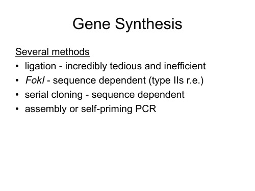
Gaps Between Almost-Primes

a rXiv:152.1693v1[math.CO ]29Jan215Gaps Between Almost-Primes and a Construction of Almost-Ramanujan Graphs Adrian Dudek Mathematical Sciences Institute The Australian National University adrian.dudek@.au Abstract For all k ≥3,we show how one can explicitly construct an infinite family of k -regular graphs all of which have second largest eigenvalue satisfying the bound O (k 1/2).This resolves an open problem of Rein-gold,Vadhan and Wigderson.1Introduction In this note,we will consider a graph X with vertex set V .By a family of graphs,we mean a sequence {X m }of graphs with |V m |→∞as m →∞.We list the eigenvalues of the adjacency matrix of a graph X as λ1(X )≥λ2(X )≥···≥λ|V |(X ).Given a finite,connected,k -regular graph,it is a straightforward exercise to show that λ1=k .It is,however,of more interest to obtain upper bounds on λ2;the following theorem of Alon and Boppana [1]gives a limit on this asymptotically.Theorem 1.1.Let {X m}be a family of finite,connected,k -regulargraphs.Then lim inf m →∞λ2(X m )≥2√Thus,asymptotically,the spectral gapλ1−λ2is bounded above by k−√2k−1.The central problem in the theory,given an integer k≥3,is to construct a k-regular family of Ramanujan graphs, more precisely a sequence{X m}offinite,connected,k-regular graphs with √λ2(X m)≤2log k)In an earlier paper,the author[6]showed how one could improve on this slightly assuming the truth of the Riemann hypothesis.One starts with the explicit construction of a family of d-regular Ramanujan graphs where d is one more than a prime,and then uses the Cartesian graph product to produce a(d+1)-regular family of graphs with at least the same spectral gap.The reader should note that the new family is not necessarily Ramanujan,as we should expect an increase in the spectral gap with respect to an increase in d. We can iterate this procedure to furnish a family of k-regular graphs for any k.On the Riemann hypothesis,Cram´e r[5]proved that one can bound the difference between consecutive primes p n,p n+1withp n+1−p n=O(√In this note we resolve,without any condition,the open problem of Rein-gold,Vadhan and Wigderson viz.the following theorem.Theorem1.2.For all sufficiently large integers k,one can explicitly construct a k-regular family{X m}of graphs such that√λ2(X m)≤4qfor all m≥1,where d(n)denotes the number of divisors of n.The well-known divisor bound states thatd(n)≤n O(1/log log n),and so one immediately has the explicit construction of a(q+1)-regular family {X m}of graphs such thatλ2(X m)≤q1/2+O(1/log log q)for all m≥1.This,however,falls short of the result of Ben-Aroya and Ta-Shma.We will also need the following result of Wu[12]on almost-primes in short intervals.3Lemma2.2.Let x be sufficiently large.Then there exists an integer n in the interval(x−x101/232,x]such that the number of prime factors of n counted with multiplicity does not exceed two.The proof proceeds as follows.Given two graphs X and Y,the Cartesian product X Y is a natural way to obtain a new graph whose properties reflectthose of the original graphs.We will not need to see the general definition of this,for we are using one specific instance of the product.Consider K2,the complete graph on two vertices,that is,the graph consist-ing of two vertices connected by a single edge.Given afinite k-regular graph X,we note that X K2is obtained simply by taking X and a duplicate ofX,and connecting each vertex in X with its duplicate vertex.We will denote this particular Cartesian product by X′and note that this is a(k+1)-regular graph with twice as many vertices as X.The following result can be found in an earlier paper by the author[6]. Theorem2.3.Let X be afinite,connected k-regular graph and let X′= X K2.Thenλ2(X′)≤λ2(X)+1.(1) Therefore,one may take a k-regular family{X m}of graphs and get a (k+1)-regular family{X′m}with the same upper bound on the second largest eigenvalue.Iterating this process will give families of all degrees.Now,let k be sufficiently large,so that we can define q to be such that qhas at most two prime factors andk−k101/232<q≤k(2) where p and q are both prime numbers.By Lemma2.1,it follows that we can construct a family{X m}of q-regular graphs such thatλ2(X m)≤4√q−1+(k−q)<4References[1]N.Alon.Eigenvalues and binatorica,2(6):83–96,1986.[2]A.Ben-Aroya and A.Ta-Shma.A combinatorial construction of almost-Ramanujan graphs using the zig-zag product.STOC’08Proceedings of the40th annual ACM symposium on the theory of computing,2008.[3]A.Brouwer and W.Haemers.Spectra of graphs.Springer,2012.[4]P.Chiu.Cubic Ramanujan binatorica,(12):275–285,1992.[5]H.Cram´e r.Some theorems concerning prime numbers.Arkiv Mathematik,5:1–33,1920.[6]A.W.Dudek.Almost-Ramanujan graphs and prime gaps.European J.Combin.,43:204–209,2015.[7]A.Lubotzky,R.Phillips,and P.Sarnak.Ramanujan bina-torica,pages261–267,1988.[8]G.Margulis.Explicit group-theoretical constructions of combinatorialschemes and their application to the design of expanders and concentra-tors.Probl.Peredachi Inf.,24:51–60,1988.[9]M.Morgenstern.Existence and explicit constructions of q+1regularRamanujan graphs for every prime power b.Theory,(Ser B(62)):44–62,1994.[10]A.K.Pizer.Ramanujan graphs and Hecke operators.Bull.Amer.Math.Soc.(N.S.),23(1):127–137,1990.[11]O.Reingold,S.Vadhan,and A.Wigderson.Entropy waves,the zig-zag graph product,and new constant degree expanders.Ann.of Math, 2(155(1)):157–187,2002.[12]J.Wu.Almost primes in short intervals.Sci.China Math.,53(9):2511–2524,2010.5。