国贸英语翻译

合集下载

国贸与外贸的区别

国贸与外贸的区别国贸：国际贸易，外贸：对外贸易。

国际贸易是从整个世界的范围来说，对外贸易是从某个国家的角度来说。

但是在国内，说到这两个词，给人的感觉概念上差不多，因为我们都是从我们中国的角度来说的。

楼上的朋友有一点说得不对，出口中国的产品到国外去只是国贸或外贸的一小部分内容，国贸或外贸不止包括产品的进出口（不仅是出口而已）（或叫有形贸易），还包括无形贸易，比如技术进出口、服务贸易等。

对一个做国际贸易的新手来说，首先他本身要具备从事国际贸易所需要的素质，我认为最重要的有以下几点：1、英语水平，特别是书面的和口头的商务英语的水平，要能很好地以这两种方式跟客户很好地沟通；2、外贸业务知识，从与客户的业务谈判、接单、安排生产到安排出货、联系货代、联系相关外贸代理公司、联系银行、安排结汇，以及这期间若出现什么问题，如何跟客户、工厂及有关各方联系解决，等等；3、以上两种技能毕竟是可以在工作实践中慢慢学习的，还不是最重要的。

做一个优秀的外贸业务员最重要的素质是认真严谨负责的工作态度。

国际贸易是那种稍有疏忽就“一失足成千古恨”的行业，容不得半点马虎。

另外，就是要“知己知彼，百战百胜”。

“知己”是：一、要对公司情况、工厂情况、产品情况等要有相当的了解；二、对公司业务操作流程、工厂业务操作流程、产品生产流程等要有相当的了解。

“知彼”是：一、对客户的定货价位、定货特点、对货物的具体要求，习惯的贸易方式、付款方式、运输方式等都要有相当的了解；二、对客户本人的脾气、爱好、习惯等要有相当的了解。

具体措施：一、下到工厂车间第一线去，亲身去参与产品生产，和普通工人交朋友，不耻下问，以熟悉产品、了解生产流程及质量检验的具体要求，并且呆的时间越长越好；二、尽可能多地翻阅公司之前的资料档案，最好做必要的笔记，以了解业务流程及老客户的定货价位、定货特点、对货物的具体要求，习惯的贸易方式、付款方式、运输方式等，还有老业务员对待客户要求的方法及措施，还有函电回复的方式；三、业务上多向老业务员请教，特别是在展会上，学习他们的谈判技巧及他们对待不同客人的不同方法。

英语专业描述

英语专业描述英语专业描述英语专业学生主要学习英语语言、文学、历史、政治、经济、外交、社会文化等方面基本理论和基本知识，受到英语听、说、读、写、译等方面的良好的技巧训练，掌握一定的科研方法，具有从事翻译、研究、教学、管理工作的业务水平及较好的素质和较强能力。

以下是店铺整理的一些英语专业描述，有兴趣的亲可以来阅读一下!英语专业描述英语(English)是联合国的工作语言之一，也是事实上的国际交流语言。

英语(文字称为英文)属于印欧语系中日耳曼语族下的西日耳曼语支，由古代从欧洲大陆移民大不列颠岛的盎格鲁、撒克逊和朱特部落的日耳曼人所说的语言演变而来，并通过英国的殖民活动传播到世界各地。

由于在历史上曾和多种民族语言接触，它的词汇从一元变为多元，语法从“多屈折”变为“少屈折”，语音也发生了规律性的变化。

根据以英语作为母语的人数计算，英语是世界上最广泛的第二语言，但它可能是世界上第三大或第四大语言(1999年统计为380,000,000人)。

世界上60%以上的信件是用英语书写的，50%以上的报纸杂志是英语的。

上两个世纪英国和美国在文化、经济、军事、政治和科学上的领先地位使得英语成为一种国际语言。

英语也是与计算机联系最密切的语言，大多数编程语言都与英语有联系，而且随着互联网的形成，使得英文的使用更普及。

与英语最接近的无疑是弗里西语，这种语言现在仍然在荷兰北部弗里斯兰省中使用，大约有50万个使用者。

一些人认为低地苏格兰语是与英语接近的一个独立语言，而一些人则认为它是英语的一个方言。

苏格兰语、荷兰东部和德国北部的低地撒克逊语与英语也很接近。

其他相关的语言包括荷兰语、南非荷兰语和德语。

诺曼人于11世纪征服英格兰，带来大量法语词汇，很大程度地丰富了英语词汇。

英语专业的知识技能1.了解我国有关的方针、政策、法规;2.掌握语言学、文学及相关人文和科技方面的基础知识;3.具有扎实的英语语言基础和较熟练的听、说、读、写、译的能力;4.了解我国国情和英语国家的社会和文化;5.具有第二外国语的一定的实际应用能力;6.掌握文献检索、资料查询的基本方法，具有初步科学研究和实际工作能力。

《公共场所双语标识英文译法》第1部分道路交通

公共场所双语标识英文译法English Translation of Public Signs第1部分：道路交通Part 1: Road Signs1 范围DB11/T 334本部分规定了北京市道路交通双语标识英文译法原则。

本部分适用于北京市道路交通中英文标识。

2 规范性引用文件下列文件中条款通过本部分引用而成为本部分条款。

凡是注日期引用文件，其随后所有修改单（不包括勘误内容）或修订版均不适用于本部分,然而，鼓励根据本部分达成协议各方研究是否可使用这些文件最新版本。

凡是不注日期引用文件，其最新版本适用于本部分。

GB/T 16159-1996 汉语拼音正词法基本规则3 术语和定义下列术语和定义适用于本部分。

3.1地名place names人们对各个地理实体赋予专有名称。

3.2地名专名specific names and terms地名中用来区分各个地理实体词。

3.3地名通名common names and terms地名中用来区分地理实体类别词。

4 总则4.1 道路交通双语标识英文译法应符合国际惯例，遵循英语习惯（见附录A）。

4.2 本部分汉语拼音用法应符合GB/T 16159要求。

5 细则5.1 警告提示信息警告提示信息翻译应按照国际惯例，遵循英语习惯，如爬坡车道Steep Grade。

5.2 地名通名5.2.1 一般（基本）规定地名通名通常采用英文直接翻译，英文单词首字母大写，其余小写。

5.2.2 街5.2.2.1 Avenue (Ave) 仅用于长安街CHANG’AN Ave，平安大街PING’AN Ave和两广路LIANGGUANG Ave。

5.2.2.2 街、大街译为Street (St)，如隆福寺街LONGFUSI St，惠新东街HUIXIN East St；西单北大街XIDAN North St，菜市口大街CAISHIKOU St。

5.2.2.3 小街、条、巷、夹道一般情况下译为Alley，当路宽达到一定规模时可译为St，如东直门北小街DONGZHIMEN North Alley，横一条HENGYITIAO Alley，东四十条DONGSI SHITIAO St，后海夹道HOUHAI Alley；斜街译为Byway。

英语专业和商务英语专业课程对比情况说明模板

英语专业和商务英语专业课程对比情况说明模板
英语专业包含商务英语专业商务英语专业指英语专业商务方向英语专业包含商务英语、国贸英语、英语教育等大一大二都是学习基础英语，大三分方向。

商务英语侧重商务英语翻译，就业方向是与商务英语有关的职业，包括翻译商务证件/信件、双方进行商务谈判是作为翻译员进行现场翻译、翻译药物/化妆品说明书等英语教育专业的学生主要从事教师工作，当然也一样可以从事商务英语方面的工作。

不管是哪个方向的同事英语专业，都可以从事于英语有关的一切职业，前提是具备相应证件。

只是商务英语方向的学校主要从事商务英语翻译，如果要从事英语教育，只要具备心理学、教育学和普通话证书就可以，只是在应聘是比英语教育专业的学生劣势。

同样英语教育专业的学生只要具备相应证件也可以从事商务英语方面的专业，但应聘时比商务英语专业的学生劣势。

商务英语，就是商务与英语相结合的课程，英语专业和商务英语这两者可比性不强。

英语专业概念更广泛，其中就包含了商务英语。

商务英语是以满足职场需求为目的，内容涵盖商务内容全过程，以职场人员和即将迈入职场的人员为目标，以商务活动中常用语言为重点的一门学科。

商务英语的特点主要在于其教学的专业化、口语化和较强的针对性，想自学是比较难的。

国贸专业英文文献翻译

Oil price fluctuations and their impact on the macroeconomic variables of Kuwait：a case study using a V AR modelSUMMARYIn this study，a vector auto regression model (V AR) and a vector error correction model (VECM) were estimated to examine the impact of oil price fluctuations on seven key macroeconomic variables for the Kuwaiti economy. Quarterly data for the period 1984 - 1998 were utilized. Theoretically and empirically speaking，VECM is superior to the V AR approach. Also，the results corresponding to the VECM model are closer to common sense.However，the estimated models indicate a high degree of interrelation between major macroeconomic variables. The empirical results highlight the causality running from the oil prices and oil revenues，to government development and current expenditure and then towards other variables. For the most part，the empirical evidence indicates that oil price shocks and hence oil revenues have a notable impact on government expenditure，both development and current. However，government development expenditure has been influenced relatively more.The results also point out the significance of the CPI in explaining a notable part of the variations of both types of government expenditure. On the other hand，the variations in value of imports are mostlyaccounted for by oil revenue fluctuations and then by the fluctuation in government development expenditures. Also，the results from the VECM approach indicate that a significant part of LM2 variance is explained by the variance in oil revenue. It reaches about 46 percent in the 10th quarter，even more than its own variations.KEY WORDS：vector auto regression (V AR); oil fluctuation; Kuwait1. INTRODUCTIONThe post-1973 effects of the oil boom on the economies of Arab oil producing countries have been diverse，though on balance，many of those governments might look back on the period 1973 –1986 as a mixed blessing. Income on the oil account certainly rose rapidly，but so did price inflation，wage rates and reliance on foreign labor. Above all，the growth of the oil sector as a contributor to national income tended to reduce the role of nonoil sectors to insignificance in most Arab states of the Gulf. This phenomenon has been termed in the literature ‘the Dutch Disease ’ . Dramatic ris es in per capita income were the fruits of rising oil revenues alone，even in the case of the larger more diversified economies of the Gulf such as Iran (Al-Abbasi，1991).There is a great deal of theoretical and empirical literature scrutinizing various aspects of the Dutch Disease economies such as Cordon and Neary (1982)，Hamilton (1983)，Neary and van Wijnbergen (1986)，Fardmanesh (1991)，Van Wijnbergen (1984)，Gelb and Associates (1988) and Taylor et al. (1986) to name a few. Recently，several empirical studies have been published on Arab oil producing countries. For instance，Taher (1987) studied the impacts of changes in the world oil prices on the different sectors of the Saudi economy. Furthermore，Al-Mutawa (1991) and Al-Mutawa and Cuddington (1994) analysed the effects of oil shocks and macroeconomic policy changes for the UAE. The results showed that，in the case of UAE，an oil-quantity boom led to higher welfare gains than an oil-price boom. Moreover，an oil-price or quantity bust always led to lower economic growth and created a welfare loss. Also，Al-Mutairi (1993) attempted to identify the sources of output fluctuations and the dynamic response of the economy to changes in key macroeconomic variables for Kuwait. His empirical results suggested that for short horizons of one and two years，shocks to the oil price account for more than 50 per cent of the variance of GDP. However，at longer horizons of three years and more，these shocks are seen to be unimportant in inducing GDP fluctuations，accounting only for less than 10 per cent of the variance. Shocks of real-government expenditure were also found to have a significant role in causing GDP fluctuations.Kuwait is a typical example of an oil-based economy. The oil sector contributes over two-thirds of GDP and over 90 per cent of exports. Although Kuwait tries hard to lessen its dependence on oil through the development of a non-oil sector，its success has so far been，at the best，very modest. The real problem is that oil prices and hence oilrevenues are exogenously determined. As a member of OPEC，Kuwait has no control over the price of its crude oil and at least theoretically speaking cannot exceed its assigned production quota. The objectives of this study are to investigate the impacts of oil price fluctuations on key macroeconomic variables of the Kuwaiti economy，to examine the direction of causality and to determine the significance of such impacts. This will certainly enhance our understanding of how international oil price fluctuations impact key macroeconomic variables and the dynamic response of these economic variables，including policy variables such as government expenditure and money supply.In this study，the analysis is carried out using two different models，namely，the vector autoregres-sion model (V AR) and the vector error correction model (VECM). The V AR technique is appropriate in this case because of its ability to characterize the dynamic structure of the model as well as its ability to avoid imposing excessive identifying restrictions associated with different economic theories. The use of V AR in macroeconomics has generated much empirical evidence，giving fundamental support to many economic theories (see Blanchard and Watson，1984，Bernanke，1986 among others).In the next section，a brief review of the literature is presented followed by the V AR model along with the data utilized. The empirical results and their interpretation are given in section four，followed by the conclusions.2. THE MODEL2.1. The background of V AR methodologyThe V AR system is based on empirical regularities embedded in the data. The V AR model may be viewed as a system of reduced form equations in which each of the endogenous variables is regressed on its own lagged values and the lagged values of all other variables in the system. An n variable V AR system can be written asA(l)Y t=A+U t(1)A(l)=l-A1l-A2l2-A m l m(2)where Y t is an n × 1 vector of macroeconomic variables，A is an n ×1 vector of constraints，and U t is an n ×1 vector of random variables，each of which is serially uncorrelated with constant variance and zero mean. Equation(2) is an n × n matrix of normalized polynomials in the lag operator l with the first entry of each polynomial on A ' s being unity.Since the error terms (U t) in the above model are serially uncorrelated，an ordinary-least-squares (OLS) technique would be appropriate to estimate this model. However，before estimating the parameters of the model A(l) meaningfully，one must limit the length of the lag in the polynomials. If l is the lag length，the number of coefficients to be estimated is n(nl +c)，where c is the number of constants.In the V AR model above，the current innovations (U t) are unanticipated but become part of the information set in the next period.This implies that the anticipated impact of a variable is captured in the coefficients of lagged polynomials while the residuals capture unforeseen contem-poraneous events. Therefore，an important feature of the V AR methodology is the use of the estimated residuals，called V AR innovations，in dynamic analysis. Unlike in conventional economic modelling，these V AR innovations are treated as an inherent part of the system.In order to analyse the impact of unanticipated policy shocks on the macroeconomic variables in a more convenient and comprehensive way，Sims (1980) proposed the use of impulse response functions (IRFs) and forecast error variance decompositions (FEVDs). IRFs and FEVDs are obtained from a moving average representation of the V AR model [Equations (1) and (2)] as shown belowY t=Constant+H t(l)U (3)AndH(l)=I+H t l+H2l (4)Where H is the coefficient matrix of the moving average representation which can be obtained by successive substitution in Equations (1) and (2). The elements of the H matrix trace the response over time of a variable i due to a unit shock given to variable j. In fact，these impulse response functions will provide the means to analyse the dynamic behaviour of the macroeconomic variables due to unanticipated shocks in the exogenous variables.Having derived the variance-covariance matrix from the moving-average representation，the FEVDs can be constructed.FEVDs represent the decomposition of forecast error variances and therefore give estimates of the contributions of distinct innovations to the variances. Thus，they can be interpreted as showing the portion of variance in the prediction for each variable in the system that is attributable to its own innovations and to shocks to other variables in the system.2.2. Vector error correction methodology Dickey and Fuller (1979) have emphasized the necessity of analysing the time-series properties of the variables before their relationship can be established. This is necessary because if the variables in question are nonstationary，then the estimated equations will yield spurious and misleading regression results. If the variables in a relationship are stationary then it is generally true that any linear combination of these variables is said to be cointegrated. Johansen’s test (1991，1995) is commonly used to test for cointegration between more than two time series. It also provides estimates of the possible long-term relationships，i.e. the parameters of the relationships that ensure cointegration. In this study，a vector error correction model (VECM) was also estimated.The VECM is basically a V AR system that builds on Johansen ' s test for cointegration and is usually referred to in the literatures as the restricted V AR.2.3. The estimated model and dataThe first step in estimating a V AR model is to make a choice of the macroeconomic variables that are essential for the analysis. Thevariables consist of one external shock measured by innovations in the price of Kuwaiti blend crude oil，three key macroeconomic variables，oil revenues，the consumer price index，(CPI) and the value of imports and three policy variables，Money Supply M2，government current expenditure and government development expenditure. The notations of these variables are as follow：OILP = Oil Price of Kuwaiti Blend CrudeOILR= Oil RevenueEXDEV = Government Development ExpenditureEXCON =Government Current ExpenditureCPI = Consumer Price IndexM2 =Money Demand (M2 Definition)IMPORTS = Value of Imports of Goods & ServicesQuarterly data for the period 1984：1-1998：4 were utilized in this study. The data for the period of the Iraqi occupation and the liberation of Kuwait were removed from the time series for obvious reasons (1990-1991). All data are from the Quarterly Monetary Statistics of the Central Bank of Kuwait and OPEC’s Monthly Bulletin. Similar to the previous studies，all the variables are expressed in logarithmic form. This can be partially justified by the fact that logarithmic forms tend to reduce the scale of the variables，which is a desirable quality when analysing the time-series properties of the variables before their relationship can be established. It is also a useful tool in providing estimates of the possible long-term relationships，i.e. the parameters of the relationships that ensure co-integration.A very important point that should be mentioned here is that the major shortcoming of the V AR approach is its lack of theoretical substance (Cooly and LeRoy，1985; Leamer，1985). In response to this criticism，Blanchard and Watson (1984) and Bernanke (1986) developed procedures，called the structural vector autoregression (SV AR) approach，which combines the features of the traditional structural modelling with those of the V AR methodology. The major advantage of using SV AR comes from the fact that standard V AR disturbances are generally characterized by contemporaneous correlations. In the presence of such correlations，the response of the system，indicated by IRFs，to an innovation in one of the variables is in fact the response to innovations in all those variables that are contemporaneously correlated with it. Similarly，the ability of FEVDs to quantify the relative contributions of specific sources of variation is confounded in the presence of this correlation. However，in standard V AR methodology this contemporaneous correlation is purged by the Cholesky orthogonalization procedure. For the most part，the Cholesky procedure implicitly assumes recursivity in the V AR model as it is estimated. Although theoretical considerations may help in determining this ordering and ex-post sensitivity analysis may further help provide insights regarding appropriate ordering，it remains largely at the discretion of the modeller.The following ordering of equations was adopted in this study; LOILP，LOILR，LEXEDEV，LEXCON，LCPI，LM2 andLIMPORTS. Generally speaking，this ordering reflects the fact that oil prices have an influence on oil revenues and then on all the other variables in the model. However，the behavior of oil prices and to some extent oil revenue are the least determined by other variables included in the model. This is quite a plausible assumption because the oil prices and hence oil revenues which consist of oil export revenues and net factor income from abroad are largely determined by the world market conditions rather than within the Kuwaiti Economy. Similarly，this ordering assumes that the government expenditure is largely determined by the level of oil revenues which again is quite a plausible assumption considering the dominant role of the public sector in driving the Kuwaiti economy. It is also sensible to assume that the value of imports is largely dependent on the level of government expenditure.Since the only variables included are those suggested by economic theory，and since theoretical considerations are important in selecting the ordering used here，the SV AR is not followed in this study. Nevertheless，the approach utilized here can be considered to be in the spirit of the SV AR approach.3. THE EMPIRICAL RESULTSFirst，the V AR technique requires stationary data，thus each series should be examined for stationarity. Table I gives the nonstationary test for all the time-series，using the conventional Dicky-Fuller test (DF)，its augmented version (ADF) and Phillips-Parron t-tests. Thesetests include a constant but no time trend，as recommended by Dickey and Fuller (1979).First，the reported t-statistics，when compared with the critical values obtained by Engle and Yoo (1987)，indicate that almost all the series，except CPI，M2 and IMPORTS，are stationary in the levels as shown by the DF，ADF and Phillips-Perron t-tests. These tests are reapplied after differencing all terms. The t-statistics on the lagged first-difference terms indicate that，for all series the null hypothesis is rejected，that is to say，all series are first differences stationary. However，in transforming a variable，a usual question arises as to whether one should use the variables in the system in levels or in differences. The overall guideline is that if there are k number of cointegrating vector among the variables used in the system，then V AR could be modelled with k stationary and n-k differences of original variables. But if all the variables in the system are nonstationary，using a V AR in levels is appropriate. On the other hand，estimating a V AR in the levels in the case of cointegration may lead to the omission of important constraints.In this context，Doan et al. (1984) noted that differencing a variable is ‘important ' in the case of Box-Jenkins ARIMA Modelling. Doan et al. also observed that it is not desirable to do so in V AR models. Fuller (1976) has also shown that differencing the data may not produce any gain so far as the ‘asymptotic efficiency’of the V AR is concerned ‘even if it is appropriate’.Moreover，Fuller has argued that differencing a variable ‘ throws information away ' while producing nosignificant gain. Thus，following Doan and Fuller’s argument，the level rather than the difference was utilized here.Second，the estimation of a V AR model requires the explicit choice of lag length in the equations of the model. Following Judge et al. (1988) and McMillin (1988)，Akaike’s AIC criterion is used to determine the lag length of the V AR model. The chosen lag length is one that minimizes the following：AIC(n)=Indet∑+(2d2n)/Twhere d is the number of variables in the model，T the sample size and∑n an estimate of the residuals’variance-covariance matrix ∑n obtained with a V AR (n). The maximum lag length is set at five quarters，considering the sample size and number of variables in the model. A maximum lag of greater than five quarters would reduce the degrees of freedom for estimation unacceptably. The result of employing this technique is summarized in Table II，which shows the corresponding AIC values. It can be seen that the AIC criterion is minimized for order 4. This suggests that，for this study，the V AR model should be of order 4.The next step is to estimate the V AR. The estimates along with their t-values are reported in Table III. Although the estimates of individual coefficients in V AR do not have a straightforward interpretation，a glance at the table generally shows that most of the t-values are significant (except for the CPI equation) and almost all of the equations have high R-squares. It also confirms the assertion that oil prices are exogenously determined than other variables included in themodel. However，oil revenue equation has a larger number of significant t-values than current expenditure and CPI.3.1. Variance decompositionTable IV presents the variance decomposition for the 10-quarters forecasts. Table IV shows that initially the variations in all of the variables are typically explained by the variables’ own trends. That is to say，at the beginning，the historical trend of each variable explains a large part of its own variations. For the most part，after ten quarters，about 60 per cent of the variance in oil prices is explained by the variable itself which is indicative of its exogenous nature. On the other hand，oil revenue explained about 93 per cent of its own variations at the first quarter and about 20 percent at the 10th quarter. Moreover，variation in oil prices account for about 45 per cent of the variation in oil revenues starting at the second quarter and through to the tenth. This shows that the causality is running from oil prices to oil revenues. Similar results are also evident for government development and current expenditures. Over a time period，about 15-17 per cent of the variance in government expenditures (development and current) is accounted for by the variations in the oil revenues.Furthermore，looking at the variance decomposition in the government expenditures (development and current) it is observed that following their own variations and oil revenues，the LCPI account for a notable part of the expenditures’ variance. The CPI accounts for onefifth of the current expenditure variations and about 15 per cent of the development expenditure. This is quite a plausible result and very apparent in the case of current expenditure.On the other hand，it is worth noting that the other variable that also picks up a significant part of the variations in government development expenditure is the value of imports. It accounts for about 16 per cent.Looking at the variance decomposition of M2，it is apparent that a noticeable part of its variance is explained by the variance in the CPI (about 33 per cent)，even more than its own variations. Also，oil prices and oil revenue，respectively，account for about 23 and 13 per cent of its variations. These results suggest an important role for money supply.Moreover，over the time period，the results show that 25-45 per cent of the variance in the value of imports is accounted for by the variation in oil revenues alone. Other variables included in the model that exert significant influence on the behaviour of imports are the two types of government expenditure but in particular，the development expenditure.3.2. Impulse responsesFigure 1 displays the Impulse Response Functions，which are essentially the dynamic multipliers .Since the primary interest is to see the response of major macroeconomic variables to the shocks given to the oil revenues and then to the government expenditure，only tentime periods are reported. An inspection of Figure 1 reveals that innovation in the oil prices and hence oil revenue has a similar effect on most of the variables in the model. Generally，most of these variables show an increase in the first quarter. This increase continues in the second and third quarter and then it gradually tapers off over the successive quarters. The only exceptions are the CPI and the value of imports and M2. This may be attributable to the shortcomings in the data set used to estimate the V AR. Recall that LCPI，LM2 and LIMPORTS were found to be non-stationary in the level.3.3. Estimation of the vector error correction model Since most of the variables included in the model pertain to stationary time series data except LCPI，LM2 and LIMPORTS，Johansen’s test (1991，1995) was applied to check for cointegrating vectors. The test indicated that there are four cointegrating vectors. Therefore，a vector error correction model is warranted. A vector error correction model is a V AR that build-in cointegration. Each co-integrating equation adds the parameters associated with the term involving levels of the series which needs to be added to each equation in the V AR. There is a sequence of nested models in this framework. The Johansen test procedure computes the likelihood ratio for each added co-integrating equation.On the basis of Johansen’s test，a Vector error correction model (VECM) was estimated. Four co-integrating equations were estimated using the same seven variables that were used in the V AR. However，since the results of estimating the VECM do not have a direct interpretation，they are not reported here.3.4. Variance decompositionThe variance decomposition results corresponding to the estimated VECM are presented in Table V. They are based on the same ordering as was used in the V AR. Comparing these results with the V AR shows that while the qualitative nature of macroeconomic linkages remains almost the same，the intensity of interaction between the variables is significantly higher when co-integration has been accounted for. For example，looking at the variance decomposition of the oil revenues，it shows that variables like government development and current expenditures have a substantially larger share when compared with the V AR results which increased from 14 per cent to about 40 percent. Similarly，the oil revenue has picked up a relatively larger proportion of the variation in the government current expenditure as well as the value of imports，especially during the first 4-6 quarters. However，the results indicate that variations in LCPI，LM2 and LIMPORTS，after 7-10 quarters，are mainly explained by changes in oil revenue alone.In particular，the variance decomposition of LM2 indicates that a significant part of its variance is explained by the variations in oil revenues (about 46 per cent after 10 quarters)，even more than its own variations. On the other hand，contrary to the result from V AR，LCPI accounts for only 7 per cent.Empirically speaking，the VECM model shows a relatively higher degree of statistical significance. Theoretically speaking，this is because it yields a closer interaction between macroeconomic variables than what the V AR indicated.3.5. Impulse response functionsFigure 2 displays the impulse response functions corresponding to the VECM model. Figure 2 indicates that innovations in the oil prices and oil revenue have a similar impact on the variables included in the model. However，similar to the V AR，most of the variables show an increase for the first few quarters then it gradually tapers off over the successive quarters with the exception of CPI，value of imports and LM2.Comparing these IRFs with those corresponding to the V AR version reveals that it takes a little longer for the multipliers in the VECM version to reach the level of the V AR version. While they generally reached their peak in the V AR version in about 6-7 quarters，it took them 8-9 quarters to reach almost the same level in the VECM version.4. CONCLUSIONS AND SOME POLICYIMPLICATIONSThe primary goal of this paper was to investigate how macroeconomic variables react to fluctuations in the world oil prices. Therefore，two different versions have been estimated，namely，the V AR and the VECM. While the qualitative nature of macroeconomiclinkages remains almost the same in the two models，the intensity of interaction between the variables is significantly higher when cointegration has been accounted for. Thus，quantitatively the two models give results that are significantly different from each other. However，empirically，the VECM gives better results because it yields a closer interaction between macroeconomic variables than by the V AR estimation. The results corresponding to the VECM are also closer to common sense.Nevertheless，the two versions estimated indicated a notable degree of interrelation between the major macroeconomic variables. The results have highlighted the causality running from oil prices towards oil revenues and then towards government expenditure and other variables. However，further assessment of the relationship between these variables，based on orthogonal innovations，lead us to believe that oil price shocks do impact macroeconomic variables in Kuwait and in particular，via government development and current expenditures.The evaluation of the decomposition of the variance of government expenditures suggests that oil revenue fluctuations account for a notable part especially in the case of development expenditure.This result is not surprising and is actually consistent with what is expected in a country in which the government is the sole owner of the main national income source，the oil and gas industry. Thus，government expenditure becomes the major determinant of the level of economic activity and the mechanism by which the government caneffect the circular flow of income within the economy.What is surprising，however，is that one would expect the impact of oil shocks to be much stronger and in particular，in the case of current government expenditure. However，this may be explained by the fact that over the last three decades，the government has accumulated capital reserve (surplus) which is regularly used to finance current government commitments，especially in times of low oil revenue.Moreover，the results also point out the significance of the CPI in explaining a notable part of the variations of both types of government expenditure. On the other hand，the variations in value of imports are mostly accounted for by oil revenue fluctuations and then by the fluctuation in government development expenditures. These results suggest that fiscal policy appears to be effective in Kuwait as the oil shocks impact government expenditure and then government expenditure accounts for a relatively considerable part of the CPI and the value of import variations.However，the results from VECM approach indicate that a significant part of LM2 variance is explained by the variance in oil revenue. It reaches about 46 per cent in the 10th quarter even more than its own variations.This exercise has shown a high degree of sensitivity of the results to specification of the variables，i.e. the theoretical structure underlying the V AR. Part of this sensitivity may be attributable to shortcomings in the data set. However，for the most part，it reflects the limitations of。

2016年对外经济贸易大学英语翻译硕士MTI考研真题及答案——英语翻译基础【精选】

词汇翻译（30分）英译汉：从10个terms 里面挑5个translate and define them briefly in Chinese (共15分，一个3分）1 added value tax增值税增值税是以商品（含应税劳务）在流转过程中产生的增值额作为计税依据而征收的一种流转税。

从计税原理上说，增值税是对商品生产、流通、劳务服务中多个环节的新增价值或商品的附加值征收的一种流转税。

实行价外税，也就是由消费者负担，有增值才征税没增值不征税。

2 annual financial report年度财务报告年度财务报告是指年度终了对外提供的财务报告。

通常将半年度，季度和月度财务报告统称为中期财务会计报告。

年度财务报告作为综合反映企业单位年末财务状况、全年经营成果和现金流量的报告，在沟通企业单位管理层与财务会计报告使用者之间起着十分重要的桥梁作用。

3 bull market牛市，旺市；多头市场。

牛市，旺市指交易旺盛的市场形势，和"淡市'相对。

多头市场又称买空市场，是指股价的基本趋势持续上升时形成的投机者不断买进证券，需求大于供给的市场现象。

4 11 2016284 law of diminishing marginal returns 边际收益递减规律又称边际效益递减规律，或边际产量递减规律，指在短期生产过程中，在其他条件不变（如技术水平不变）的前提下，增加某种生产要素的投入，当该生产要素投入数量增加到一定程度以后，增加一单位该要素所带来的效益增加量是递减的，边际收益递减规律是以技术水平和其他生产要素的投入数量保持不变为条件的条件下进行讨论的一种规律。

5 angel investment天使投资是权益资本投资的一种形式，是指富有的个人出资协助具有专门技术或独特概念的原创项目或小型初创企业，进行一次性的前期投资。

它是风险投资的一种形式，在根据天使投资人的投资数量以及对被投资企业可能提供的综合资源进行投资。

关于道路交通名称的英语翻译

关于道路交通名称的英语翻译Part 1: Road Signs1 范围DB11/T 334的本部分规定了北京市道路交通双语标识英文译法的原则。

本部分适用于北京市道路交通中的英文标识。

2 规范性引用文件下列文件中的条款通过本部分的引用而成为本部分的条款。

凡是注日期的引用文件，其随后所有的修改单（不包括勘误的内容）或修订版均不适用于本部分,然而，鼓励根据本部分达成协议的各方研究是否可使用这些文件的最新版本。

凡是不注日期的引用文件，其最新版本适用于本部分。

GB/T 16159-1996 汉语拼音正词法基本规则3 术语和定义下列术语和定义适用于本部分。

3.1地名place names人们对各个地理实体赋予的专有名称。

3.2地名专名specific names and terms地名中用来区分各个地理实体的词。

3.3地名通名common names and terms地名中用来区分地理实体类别的词。

4 总则4.1 道路交通双语标识的英文译法应符合国际惯例，遵循英语习惯（见附录A）。

4.2 本部分汉语拼音用法应符合GB/T 16159的要求。

5 细则5.1 警告提示信息警告提示信息的翻译应按照国际惯例，遵循英语习惯，如爬坡车道Steep Grade。

5.2 地名通名5.2.1 一般（基本）规定地名通名通常采用英文直接翻译，英文单词首字母大写，其余小写。

5.2.2 街5.2.2.1 Avenue (Ave) 仅用于长安街CHANG’AN Ave，平安大街PING’AN Ave和两广路LIANGGUANG Ave。

5.2.2.2 街、大街译为Street (St)，如隆福寺街LONGFUSI St，惠新东街HUIXIN East St；西单北大街XIDAN North St，菜市口大街CAISHIKOU St。

常用服装英文（摘自穿针引线）

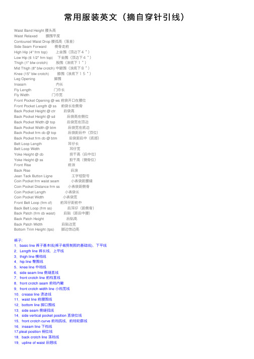
常⽤服装英⽂（摘⾃穿针引线）Waist Band Height 腰头⾼Waist Relaxed 腰围平度Contoured Waist Drop 腰弧⾼（落差）Side Seam Forward 侧⾻⾛前High Hip (4" frm top) 上坐围（顶边下４＂）Low Hip (6 1/2" frm top) 下坐围（顶边下４＂）Thigh (1" blw crotch) 股围（浪底下１＂）Mid Thigh (8" blw crotch) 中腿围（浪底下８＂）Knee (15" blw crotch) 膝围（浪底下１５＂）Leg Opening 脚围Inseam 内长Fly Length 门⼱长Fly Width 门⼱宽Front Pocket Opening @ ws 前袋开⼝在腰位Front Pocket Length @ ss 前袋长在侧⾻Back Pocket Height @ ctr 后袋⾼Back Pocket Height @ sd 后袋⾼在侧位Back Pocket Width @ top 后袋宽在顶边Back Pocket Width @ btm 后袋宽在底边Back Pocket frm cb @ top 后袋距后中（顶位）Back Pocket frm cb @ btm 后袋距后中（底部）Belt Loop Length ⽿仔长Belt Loop Width ⽿仔宽Yoke Height @ cb 担⼲⾼（后中位）Yoke Height @ ss 担⼲⾼（侧⾻位）Front Rise 前浪Back Rise 后浪Jean Tack Button Ligne ⼯字钮型号Coin Pocket frm waist seam ⼩表袋距腰缝Coin Pocket Distance frm ss ⼩表袋距侧⾻Coin Pocket Length ⼩表袋长Coin Pocket Width ⼩表袋宽Front Belt Loop (frm cf) 前⽿仔距前中Back Belt Loop (frm ss) 后⽿仔（距侧⾻）Back Patch (frm cb waist) 后贴（距后中腰）Back Patch Height 后贴⾼Back Patch Width 后贴边宽Bottom Trim Height (tps) 脚边饰边⾼裤⼦:1．basic line 裤⼦基本线(裤⼦裁剪制图的基础线)，下平线2．Length line 裤长线，上平线3．thigh line 横裆线4．hip line 臀围线5．knee line 中裆线6．side seam line 侧缝直线7．front crotch line 前裆直线8．front crotch seam 前裆内撇9．front crotch width line ⼩裆宽线10．crease line 烫迹线11．waist line 前腰围线12．bottom line 脚⼝围线13．side seam 侧缝弧线14．side vertical pocket position 直袋位线15．front crotch curve 前裆弧线，前裆轮廓线16．inseam line 下裆线17.pleat position 裥位线18．back crotch line 落裆线19．upline of waist 后翘线20．back waist seam 后腰缝线21．curve width line of back crotch seam 后裆宽线22．back crotch curve 后档弧线，后裆缝轮廓线23．waist dart 后省线24．hip pocket position line 后袋线25．waistband roll line 腰头上⼝线26．waistband neckline 腰头下⼝线27．fly facing edge 门襟⽌⼝线28．fly facing outside edge 门襟外⼝线29．fly shield inside edge ⾥襟⾥⼝线30．fly shield outside edge ⾥襟外⼝线Double – breasted双纽襟Braid 缀以线辫纽Buckled 带扣Fly 暗纽襟Crossed –over 叠门襟Frogging 纺锤形纽扣Knotted tie 缚结物Laced – up 系紧绳带Linked 连接饰物Looped 结环纽眼Side –buttoned 侧边纽门Single buttoned 单边纽扣Strap 条扣Tab 扣绊Bow 蝴蝶结Three –button grouping 3粒组纽Toggled 索结绳纽Wraped& tied 叠襟系带Zipper 拉链怎样做外贸服装英⽂做⼀名外贸服装英⽂跟单,⼀般都要具备以下条件:1.⼤专以上学历,英语/国贸/纺织服装专业优先,**级以上.2.⼀年以上⼯作经验,有同类产品(针织\梭织\⽑织)⼯作经验优先.如果以上两个条件您都不适合的话,或者您有相关⼯作经验但不全⾯,那么,别失望,让我们来看看⾯试时⼈事经理和您未来的BOSS问得最多的⾼频问题:⾯试⼈:请说说跟单的⼯作流程.应聘者:完整的⼯作流程就是从接单到出货,每⼀个环节都要跟进.详细来说,客⼈会先发⼀份tech-pack给⼯⼚打版(sample).先做头版(proto sample)给客批,批了之后做fit版(fit sample),有fit版做表⽰客⼈有意向下⼤货订单.批了fit办之后,就做产前版(Per-Production sample),也就是常说的PP版. 客⼈批了PP版,这条版的⾝份就是⽣产版.可以⽤来参考⽣产⼤货⽤.接下来跟进⼤货⽣产进度,何时有布/物料,何时开裁,何时车缝,何时洗⽔,何时包装,何时出货,作为⼀名跟单员,這些都应该知道.⾯试⼈:版和⼤货在⽣产中预到问题应该怎样处理?应聘者:这要看情况⽽定,如果是客资料的问题导致样版或⼤货做错,需与客⼈沟通,是接受还是返做.如果是⼯⼚内部⼯作失误,则应该找回相关负责⼈,看是否有措施可以补救.⽆法补救⼜不够时间返做,需与客⼈沟通,申请延期.最常见的问题是尺⼨超出客⼈接受范围.解决⽅法有,尺⼨偏⼩做拉烫,尺⼨偏⼤做缩烫.特别⼤⽆法缩烫的,可以拆了修剪⼩后重车.尺⼨太⼩只能重裁.⼤貨可以改碼,補裁部分.⼩贴⼠:实际上,⾯试时⼤部分问题都已在简历上定清楚了,如学历/英⽂⽔平/⼯作经验呀,等等,⾯试主要是看看你的实际操作与表达能⼒怎么样.如果你对服装专业知识了解太少的话,建议看看以下笔试题.****************************************************************************************以下是⽜仔裤中英⽂尺⼨对照翻译.也是跟单员笔试最常见的考试题⽬.WB Height 腰⾼Waist Relaxed at top edge 腰阔顶边度Waist Relaxed at bttm edge 腰阔底边度Fly/J-Stitch Length 鈕牌J线长Low Hip Plcmnt from Bottom WB Seam 下坐围位置腰底下Low Hip - 3pt 下坐围三点度Thigh 1" from Crotch 脾围浪下1"Mid Thigh 6" from Crotch 中脾浪下6"Knee 12" from Crotch 膝围浪下12"Leg Opening 脚围Inseam - 34" 248802 内长 34" 248802Fly/J-Stitch Width 鈕牌J线阔Zipper Length 拉链长Front Rise from WB Seam - striaght 前浪腰底直度(不包腰)Back Rise from WB Seam - striaght 后浪腰底直度(不包腰)Front Pocket Opening at Outseam from WB Seam(Bottoms) 前袋开⼝侧⾻度Front Pocket Opening along WB Seam 前袋开⼝腰底度Back Yoke Height at CB 机头后中⾼Back Yoke Height at SS 机头侧⾻⾼Back Pocket from CB 后袋由后中Back Pocket from Yoke Seam - Near Outseam 后袋距机头⾻近侧⾻Back Pocket from Yoke Seam - Near CB 后袋距机头⾻近后中Back Pocket Width at Top 后袋顶阔Back Pocket Width at Bottom 后袋底阔Back Pocket Length at Point 后袋中⾼Back Pocket Length at Side 后袋侧⾼Coin Pocket Width at Top- 表袋顶阔Coin Pocket from WB Seam 表袋由腰底Coin Pocket over from side seam 后袋由侧⾻Belt Loop Length ⽿仔长Belt Loop Width ⽿仔阔Total number of belt loops ⽿仔数Side seam topstitch length blw wb 保险线长(英⽂的本意是侧⾻间线长腰下,即保险线)Inseam 32" 251171 内长 32" 251171Inseam 30" 258127 内长 30" 258127****************************************************************************************以下是客⼈批版评语翻译举例.这是必需学习的内容.PP FIT COMMENTS - 13/09/10Size 10;-- Reduce waist by 1cm to measure 41cm.腰減1cm⾄41cm.- Low hip ok as sample at 52cm.下坐圍接受如辦52cm.- All other M'ments are ok to spec.其它尺⼨接受.Size 14;-- Reduce waist by 1cm to measure 46cm.腰減1cm⾄46cm.- Reduce hip in accordance to size 10, to measure 57cm.下坐圍相應sz 10做57cm.- All other M'ments are ok to spec.其它尺⼨接受.Trims / Make;-- Ensure hem stich is neat and straight and stitch tension not tight.確保腳⾞線整⿑和直及線步不要緊.- Back welt pocket depth must be consistant.后唇袋⾼度要⼀⾄.- The button size is too large; Please reduce to 28Ligne.鈕号太⼤, 要改做28L.- The button quality is incorrect! Must be same as per approved Boys Walter / Barry. Please check and esnure correct.鈕款要和walter & barry⼀樣.APPROVED WITH COMMENTS. PLEASE SUBMIT 1 X 10 AND 1 X 14 PRE SHIPMENT SAMPLES.ADDITIONAL COMMENT 17/9/10- Please reduce front rise to measure 24cm excluding waistband.減前浪⾄24cm(不包括腰頭).。

1、下载文档前请自行甄别文档内容的完整性，平台不提供额外的编辑、内容补充、找答案等附加服务。
2、"仅部分预览"的文档,不可在线预览部分如存在完整性等问题,可反馈申请退款(可完整预览的文档不适用该条件!)。
3、如文档侵犯您的权益，请联系客服反馈,我们会尽快为您处理(人工客服工作时间：9:00-18:30)。

1、通过国际贸易，可以使消费者和贸易国获取本国没有的商品和服务。

通过国际贸易，富裕国家可以更高效的使用其劳动力、技术或资本等资源。

Trading globally gives consumers and countries the opportunity to be exposed to goods and services not available in their own countries. International trade allows wealthy countries to use their resources-whether labor ，technology ,or capital-more efficiently.
2、自从实行改革开放政策以后，特别是加入世界贸易组织以后，中国的对外贸易取得了引人注目的增长。

Since the implementation of reforms and opening up policy ,especially after its accession to the WTO ,China has achieved remarkable growth in foreign trade.
3、所有国家都享有公认的保护国家利益的权利，但是这个原则以及他们对世界贸易组织规则的理解都可能存在很大的差异。

All countries enjoy a recognized right to safeguard national interests ,but this principle ,as well as the interpretation of WTO rules themselves,is subject to considerable latitude in interpretation.
4、在签订许可证协议之前，许可方全面了解被许可方国家有关知识产权的法律、法规。

Before entering into a licensing agreement ,the licensor should have a thorough knowledge of the laws and regulations concerning the intellectual property rights in the licensee’s country.
5、当货物装上火车或卡车之后，或者如果是海运或空运是货物交付承运人时，卖方就不对损失承担责任。

The seller’s responsibility for costs and risks of loss will end when the rail car or truck trailer is loaded, or in the case of sea or air transport, when the goods are delivered to the carrier for loading。

6、环境条款允许一个国家限制另一个无明确环境标准国家的进口，在这方面，环境条款有些像劳工条款。

Environmental provisions allow a country to restrict imports from other countries without a clear environmental standards, then in this regard, the environmental provisions are in as much as the labor provisions.
7、一旦报价提交给买方，如果买方根据此报价订货，出口商就有责任履行所有报价上的条款。

Once the quotation has been submitted to the buyer, the exporter is committed to fulfilling all the terms contained within the document should an order be placed on the strength of it.
8、凭一流银行开立的以卖方为受益人，不可撤销、可转让、由主要货币国家一流银行保兑、含全部货款的即期信用证，连同下列单据支付。

Payment by a prime banker’s irrevocable, transferable L/C, confirmed by a first-class bank in the key currency country, covering full value of the contracted goods, in favor of seller, available by draft at sight for 100% invoice value, accompanied with the following documents.
9、我们今天已通知我方银行，开立以你方为抬头的保兑的、不可撤销的、允许分运和转船的信用证，凭即期汇票并附全套装运交易所向议付行议付。

We have today instructed our bank to open in your favor a confirmed, irrevocable letter of credit with partial shipment and transshipment allowed, available by draft at sight, against surrendering the full set of shipping documents to the negotiating bank.
10、跟单信用证是银行根据卖方的请求开立的该银行承诺凭提交有关货运单据向受益人付款的书面文书。

A documentary credit is a letter issued by a bank at the request of the seller whereby the bank promises to pay a beneficiary against presentation of documents relating to the dispatch of goods.。