公司理财--第11章
(公司理财)公司理财(精要版)知识点归纳

第一章.公司理财导论1.企业组织形态:单一业主制、合伙制、股份公司(所有权和管理相分离、相对容易转让所有权、对企业债务负有限责任,使企业融资更加容易。
企业寿命不受限制,但双重课税)2.财务管理的目标:为了使现有股票的每股当前价值最大化。
或使现有所有者权益的市场价值最大化。
3.股东与管理层之间的关系成为代理关系。
代理成本是股东与管理层之间的利益冲突的成本。
分直接和间接。
4.公司理财包括三个领域:资本预算、资本结构、营运资本管理第二章.1.在企业资本结构中利用负债成为“财务杠杆”。
2.净利润与现金股利的差额就是新增的留存收益。
3.来自资产的现金流量=经营现金流量(OCF)-净营运资本变动-资本性支出4.OCF=EBIT+折旧-税5.净资本性支出=期末固定资产净值-期初固定资产净值+折旧6.流向债权人的现金流量=利息支出-新的借款净额7.流向股东的现金流量=派发的股利-新筹集的净权益第三章1.现金来源:应付账款的增加、普通股本的增加、留存收益增加现金运用:应收账款增加、存货增加、应付票据的减少、长期负债的减少2.报表的标准化:同比报表、同基年度财报3.ROE=边际利润(经营效率)X总资产周转率(资产使用效率)X权益乘数(财务杠杆)4.为何评价财务报表:内部:业绩评价。
外部:评价供应商、短期和长期债权人和潜在投资者、信用评级机构。
第四章.1.制定财务计划的过程的两个维度:计划跨度和汇总。
2.一个财务计划制定的要件:销售预测、预计报表、资产需求、筹资需求、调剂、经济假设。
3.销售收入百分比法:提纯率=再投资率=留存收益增加额/净利润=1-股利支付率资本密集率=资产总额/销售收入4.内部增长率=(ROAXb)/(1-ROAXb)可持续增长率=ROE/(1-ROEXb):企业在保持固定的债务权益率同时没有任何外部权益筹资的情况下所能达到的最大的增长率。
是企业在不增加财务杠杆时所能保持的最大的增长率。
(如果实际增长率超过可持续增长率,管理层要考虑的问题就是从哪里筹集资金来支持增长。
公司理财罗斯中文版11
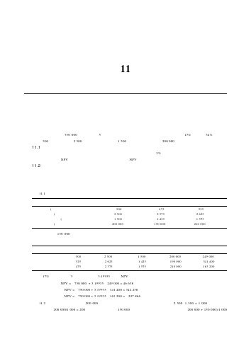
第11章项目分析与评估◆本章复习与自测题根据下列基本情况下的资料,回答本章复习与自测题中的问题。
某项目的成本为750 000美元,年限为5年,没有残值,并以直线法折旧完毕。
必要报酬率为17%,税率为34%,销售量为每年500件,单位价格为2 500美元,单位变动成本为1 500美元,固定成本为每年200 000美元。
11.1 情境分析假定你认为这里的销售量、价格、变动成本以及固定成本预测的准确度在5%以内。
这些预测值的上限和下限分别是多少?基本情况下的NPV是多少?最好的情况和最差的情况下的NPV又是多少?11.2 保本点分析给定上一题中的基本情况预测值,分别求出这个项目的现金保本点、会计保本点和财务保本点。
回答时,忽略税。
◆本章复习与自测题解答11.1 我们可以把相关资料整理如下:基本情况下限上限销售量(件)500475525单位价格(美元) 2 500 2 375 2 625单位变动成本(美元) 1 500 1 425 1 575固定成本(美元)200 000190 000210 000折旧是每年150 000美元。
因此,我们可以计算每种情境下的现金流量。
请记住,我们为最差的情况设定高成本和低价格、低销售收入,而最好的情况则正好相反。
情境销售量(件)单位价格(美元)变动成本(美元)固定成本(美元)现金流量(美元)基本情况500 2 500 1 500200 000249 000最好的情况525 2 625 1 425190 000341 400最差的情况475 2 375 1 575210 000163 200在17%的贴现率下,5年的年金系数为3.19935,因此NPV为:基本情况下的NPV = -750 000 + 3.19935×249 000 = 46 638美元最好的情况下的NPV = -750 000 + 3.19935×341 400 = 342 258美元最差的情况下的NPV = -750 000 + 3.19935×163 200 = -227 866美元11.2 在这种情况下,我们有200 000美元的现金可以弥补固定成本。
罗斯《公司理财》(第11版)笔记和课后习题详解

读书笔记模板
01 思维导图
03 读书笔记 05 作者介绍
目录
02 内容摘要 04 目录分析 06 精彩摘录
思维导图
本书关键字分析思维导图
习题
笔记
经典 书
第章
风险
预算
笔记
教材
习题 复习
收益
第版
笔记
市场
习题
定价
资本
期权
内容摘要
内容摘要
本书是罗斯的《公司理财》(第11版)(机械工业出版社)的学习辅导电子书。本书遵循该教材的章目编排, 包括8篇,共分31章,每章由两部分组成:第一部分为复习笔记;第二部分为课(章)后习题详解。本书具有以 下几个方面的特点:(1)浓缩内容精华,整理名校笔记。本书每章的复习笔记对本章的重难点进行了整理,并参 考了国内名校名师讲授罗斯的《公司理财》的课堂笔记,因此,本书的内容几乎浓缩了经典教材的知识精华。(2) 选编考研真题,强化知识考点。部分考研涉及到的重点章节,选编经典真题,并对相关重要知识点进行了延伸和 归纳。(3)解析课后习题,提供详尽答案。国内外教材一般没有提供课(章)后习题答案或者答案很简单,本书 参考国外教材的英文答案和相关资料对每章的习题进行了详细的分析。(4)补充相关要点,强化专业知识。一般 来说,国外英文教材的中译本不太符合中国学生的思维习惯,有些语言的表述不清或条理性不强而给学习带来了 不便,因此,对每章复习笔记的一些重要知识点和一些习题的解答,我们在不违背原书原意的基础上结合其他相 关经典教材进行了必要的整理和分析。
12.1复习笔记 12.2课后习题详解
第13章风险、资本成本和估值
13.1复习笔记 13.2课后习题详解
公司理财

本章目标 引导案例 第一节营运资本概述 第二节现金管理 第三节应收账款管理 第四节存货管理 第五节短期债务筹资管理 知识拓展 课后思考与练习
本章目标 引导案例 第一节股利基本理论 第二节股利政策与影响因素 第三节股利支付 知识拓展 课后思考与练习 案例分析
本章目标 引导案例 第一节企业集团财务管理概述 第二节企业集团的资金运筹管理 第三节企业集团的财务战略管理 知识拓展 课后思考与练习 案例分析
第十四章国际财务Байду номын сангаас管理
本章目标 引导案例 第一节企业组织形式 第二节公司理财目标与价值理论 第三节公司理财的主要内容 第四节公司理财的原则与职能 知识拓展 课后思考与练习 案例分析
本章目标 引导案例 第一节资金时间价值观念 第二节风险与收益权衡观念 知识拓展 课后思考与练习 案例分析
本章目标 引导案例 第一节公司理财环境概述 第二节宏观理财环境 第三节微观理财环境 知识拓展 课后思考与练习 案例分析
本章目标 引导案例 第一节资本成本 第二节杠杆效应 第三节最优资本结构的确定 知识拓展 课后思考与练习 案例分析
本章目标 引导案例 第一节项目投资概述 第二节投资项目现金流量的估计 第三节项目投资评价方法 第四节项目投资评价指标的应用 第五节风险投资决策 知识拓展 课后思考与练习
本章目标 引导案例 第一节证券投资概述 第二节债券投资 第三节股票投资 知识拓展 课后思考与练习 案例分析
目录分析
1
内容提要
2
第一章公司理 财概述
3
第二章公司理 财价值观念
4
第三章公司理 财环境
5
第四章财务分 析
第六章企业筹资规 模和方式
第五章财务预算
第七章企业筹资决 策
罗斯公司理财第九版第十一章课后答案对应版

第十一章:收益和风险:资本资产定价模型1.系统性风险通常是不可分散的,而非系统性风险是可分散的。
但是,系统风险是可以控制的,这需要很大的降低投资者的期望收益。
2.(1)系统性风险(2)非系统性风险(3)都有,但大多数是系统性风险(4)非系统性风险(5)非系统性风险(6)系统性风险3.否,应在两者之间4.错误,单个资产的方差是对总风险的衡量。
5.是的,组合标准差会比组合中各种资产的标准差小,但是投资组合的贝塔系数不会小于最小的贝塔值。
6. 可能为0,因为当贝塔值为0 时,贝塔值为0 的风险资产收益=无风险资产的收益,也可能存在负的贝塔值,此时风险资产收益小于无风险资产收益。
7.因为协方差可以衡量一种证券与组合中其他证券方差之间的关系。
8. 如果我们假设,在过去3 年市场并没有停留不变,那么南方公司的股价价格缺乏变化表明该股票要么有一个标准差或贝塔值非常接近零。
德州仪器的股票价格变动大并不意味着该公司的贝塔值高,只能说德州仪器总风险很高。
9. 石油股票价格的大幅度波动并不表明这些股票是一个很差的投资。
如果购买的石油股票是作为一个充分多元化的产品组合的一部分,它仅仅对整个投资组合做出了贡献。
这种贡献是系统风险或β来衡量的。
所以,是不恰当的。
10. The statement is false. If a security has a negative beta, investors would want to hold the asset to reduce the variability of their portfolios. Those assets will have expected returns that are lower than the risk-free rate. To see this, examine the Capital Asset Pricing Model:E(R S) = R f + S[E(R M) – R f] If S < 0, then the E(R S) < R f11. Total value = 95($53) + 120($29) = $8,515The portfolio weight for each stock is:WeightA = 95($53)/$8,515 = .5913 WeightB = 120($29)/$8,515 = .4087 12.Total value = $1,900 + 2,300 = $4,200So, the expected return of this portfolio is:E(R p) = ($1,900/$4,200)(0.10) + ($2,300/$4,200)(0.15) = .1274 or 12.74%13. E(R p) = .40(.11) + .35(.17) + .25(.14) = .1385 or 13.85%14. Here we are given the expected return of the portfolio and the expected return of each asset in the portfolio and are asked to find the weight of each asset. We can use the equation for the expected return of a portfolio to solve this problem. Since the total weight of a portfolio must equal 1 (100%), the weight of Stock Y must be one minus the weight of Stock X. Mathematically speaking, this means:E(R p) = .129 = .16w X + .10(1 –w X)We can now solve this equation for the weight of Stock X as:.129 = .16w X + .10 – .10w X w X = 0.4833So, the dollar amount invested in Stock X is the weight of Stock X times the total portfolio value, or: Investment in X = 0.4833($10,000) = $4,833.33And the dollar amount invested in Stock Y is:Investment in Y = (1 – 0.4833)($10,000) = $5,166.6715. E(R) = .2(–.09) + .5(.11) + .3(.23) = .1060 or 10.60%16. E(RA) = .15(.06) + .65(.07) + .20(.11) = .0765 or 7.65%E(RB) = .15(–.2) + .65(.13) + .20(.33) = .1205 or 12.05%17. E(R A) = .10(–.045) + .25 (.044) + .45(.12) + .20(.207) = .1019 or 10.19%方差=.10(–.045 – .1019)⌒2 + .25(.044 – .1019)⌒2 + .45(.12 – .1019)⌒2 + .20(.207 – .1019)⌒2 = .00535标准差= (.00535)1/2 = .0732 or 7.32%18. E(R p) = .15(.08) + .65(.15) + .20(.24) = .1575 or 15.75%If we own this portfolio, we would expect to get a return of 15.75 percent.19. a.Boom: E(R p) = (.07 + .15 + .33)/3 = .1833 or 18.33%Bust: E(R p) = (.13 + .03 .06)/3 = .0333 or 3.33%E(Rp) = .80(.1833) + .20(.0333) = .1533 or 15.33%b. Boom: E(R p)=.20(.07) +.20(.15) + .60(.33) =.2420 or 24.20%Bust: E(R p) =.20(.13) +.20(.03) + .60( .06) = –.0040 or –0.40%E(R p) = .80(.2420) + .20( .004) = .1928 or 19.28%P的方差= .80(.2420 – .1928)⌒2 + .20( .0040 – .1928)⌒2 = .0096820.a.Boom: E(R p) = .30(.3) + .40(.45) + .30(.33) = .3690 or 36.90%Good: E(R p) = .30(.12) + .40(.10) + .30(.15) = .1210 or 12.10%Poor: E(R p) = .30(.01) + .40(–.15) + .30(–.05) = –.0720 or –7.20%Bust: E(R p) = .30(–.06) + .40(–.30) + .30(–.09) = –.1650 or –16.50%E(R p) = .20(.3690) + .35(.1210) + .30(–.0720) + .15(–.1650) = .0698 or 6.98%b. p⌒2 = .20(.3690 – .0698)⌒2 + .35(.1210 – .0698)⌒2 + .30(–.0720 – .0698)⌒2 + .15(–.1650 – .0698)⌒2 = .03312p的标准差= (.03312)⌒1/2 = .1820 or 18.20%21. β= .25(.75) + .20(1.90) + .15(1.38) + .40(1.16) = 1.2422.βp = 1.0 = 1/3(0) + 1/3(1.85) + 1/3(βX) βX = 1.1523.E(R i) = R f + [E(R M) – R f] ×βiE(R i) = .05 + (.12 – .05)(1.25) = .1375 or 13.75%24. We are given the values for the CAPM except for the of the stock. We need to substitute these values into the CAPM, and solve for the of the stock. One important thing we need to realize is that we are given the market risk premium. The market risk premium is the expected return of the market minus the risk-free rate. We must be careful not to use this value as the expected return of the market. Using the CAPM, we find:E(R i) = .142 = .04 + .07βi 则βi = 1.4625. E(R i) = .105 = .055 + [E(R M) – .055](.73) 则E(R M) = .1235 or 12.35%26. E(R i) = .162 = R f + (.11 – R f)(1.75).162 = R f + .1925 – 1.75R f则R f = .0407 or 4.07%27. a. E(R p) = (.103 + .05)/2 = .0765 or 7.65%b. We need to find the portfolio weights that result in a portfolio with a of 0.50. We know the 贝塔of the risk-free asset is zero. We also know the weight of the risk-free asset is one minus the weight of the stock since the portfolio weights must sum to one, or 100 percent. So:c. We need to find the portfolio weights that result in a portfolio with an expected return of 9 percent. We also know the weight of the risk-free asset is one minus the weight of the stock since the portfolio weights must sum to one, or 100 percent. So:d. Solving for the of the portfolio as we did in part a, we find:18. ßp = w W(1.3) + (1 –w W)(0) = 1.3w WSo, to find the βof the portfolio for any weight of the stock, we simply multiply the weight of the stock times its β.Even though we are solving for the and expected return of a portfolio of one stock and the risk-free asset for different portfolio weights, we are really solving for the SML. Any combination of this stock and the risk-free asset will fall on the SML. For that matter, a portfolio of any stock and the risk-free asset, or any portfolio of stocks, will fall on the SML. We know the slope of the SML line is the market risk premium, so using the CAPM and the information concerning this stock, the market risk premium is:E(R W) = .138 = .05 + MRP(1.30)MRP = .088/1.3 = .0677 or 6.77%So, now we know the CAPM equation for any stock is:E(R p) = .05 + .0677*贝塔p29. E(R Y) = .055 + .068(1.35) = .1468 or 14.68%E(R Z) = .055 + .068(0.85) = .1128 or 11.28%Reward-to-risk ratio Y = (.14 – .055) / 1.35 = .0630Reward-to-risk ratio Z = (.115 – .055) / .85 = .070630. (.14 – R f)/1.35 = (.115 – R f)/0.85We can cross multiply to get: 0.85(.14 – R f) = 1.35(.115 – R f)Solving for the risk-free rate, we find:0.119 – 0.85R f = 0.15525 – 1.35R f R f = .0725 or 7.25%31.32. [E(R A) – R f]/ A = [E(R B) – R f]/ßBRP A/β A = RP B/β B βB/βA = RP B/RP A33. Boom: E(R p) = .4(.20) + .4(.35) + .2(.60) = .3400 or 34.00%Normal: E(R p) = .4(.15) + .4(.12) + .2(.05) = .1180 or 11.80%Bust: E(R p) = .4(.01) + .4(–.25) + .2(–.50) = –.1960 or –19.60%E(R p) = .35(.34) + .40(.118) + .25(–.196) = .1172 or 11.72%σp⌒2= .35(.34 – .1172)2 + .40(.118 – .1172)2 + .25(–.196 – .1172)2 = .04190σp= (.04190)1/2 = .2047 or 20.47%b. RP i = E(R p) – R f = .1172 – .038 = .0792 or 7.92%c.Approximate expected real return = .1172 – .035 = .0822 or 8.22%1 + E(R i) = (1 + h)[1 + e(r i)]1.1172 = (1.0350)[1 + e(r i)]e(r i) = (1.1172/1.035) – 1 = .0794 or 7.94%Approximate expected real risk premium = .0792 – .035 = .0442 or 4.42%Exact expected real risk premium = (1.0792/1.035) – 1 = .0427 or 4.27%34. w A = $180,000 / $1,000,000 = .18 w B = $290,000/$1,000,000 = .29βp = 1.0 = w A(.75) + w B(1.30) + w C(1.45) + w Rf(0) w C = .33655172Invest in Stock C = .33655172($1,000,000) = $336,551.721 = w A + w B + w C + w Rf 1 = .18 + .29 + .33655172 + w Rf w Rf = .19344828Invest in risk-free asset = .19344828($1,000,000) = $193,448.28w X(.172) + w Y(.0875) + (1 –w X –w Y)(.055)35. E(R p) = .1070 =βp = .8 = w X(1.8) + w Y(0.50) + (1 –w X – w Y)(0)w X = –0.11111 w Y = 2.00000 w Rf = –0.88889Investment in stock X = –0.11111($100,000) = –$11,111.1136. E(R A) = .33(.082) + .33(.095) + .33(.063) = .0800 or 8.00%E(R B) = .33(–.065) + .33(.124) + .33(.185) = .0813 or 8.13%股票A:方差=.33(.082 – .0800)⌒2 + .33(.095 – .0800)⌒2 + .33(.063 – .0800)⌒2 = .00017 标准差=(.00017)⌒1/2 = .0131 or 1.31%股票B:方差=.33(–.065 – .0813)⌒2 + .33(.124 – .0813)⌒2 + .33(.185 – .0813)⌒2 = .01133 标准差= (.01133)1/2 = .1064 or 1064%Cov(A,B) = .33(.092 – .0800)(–.065 – .0813) + .33(.095 – .0800)(.124 – .0813) + .33(.063– .0800)(.185 – .0813) = –.000472ρA,B = Cov(A,B) / (标准差A 标准差B)= –.000472 / (.0131)(.1064) = –.337337. E(R A) = .30(–.020) + .50(.138) + .20(.218) = .1066 or 10.66%E(R B) = .30(.034) + .50(.062) + .20(.092) = .0596 or 5.96%A的方差 =.30(–.020 – .1066)⌒2 + .50(.138 – .1066)⌒2 + .20(.218 – .1066)⌒2 = .00778 2 A的标准差= (.00778)⌒1/2 = .0882 or 8.82%B的方差=.30(.034 – .0596)⌒2 + .50(.062 – .0596)⌒2 + .20(.092 – .0596)⌒2 = .00041B的标准差= (.00041)⌒1/2 = .0202 or 2.02%Cov(A,B) = .30(–.020 – .1066)(.034 – .0596) + .50(.138 – .1066)(.062 – .0596)+ .20(.218 – .1066)(.092 – .0596) = .001732ρA,B = Cov(A,B) / A的标准差*B的标准差= .001732 / (.0882)(.0202) = .970138. a. E(R P) = w F E(R F) + w G E(R G)E(R P) = .30(.10) + .70(.17) = .1490 or 14.90%b. The variance of a portfolio of two assets can be expressed as:标准差= (.18675)⌒1/2 = .4322 or 43.22%39. a. The expected return of the portfolio is the sum of the weight of each asset times the expected return of each asset, so:E(R P) = w A E(R A) + w B E(R B) = .45(.13) + .55(.19) = .1630 or 16.30%c. As Stock A and Stock B become less correlated, or more negatively correlated, the standard deviation of the portfolio decreases.40.(iv) The market has a correlation of 1 with itself.(v) The beta of the market is 1.(vi) The risk-free asset has zero standard deviation.(vii) The risk-free asset has zero correlation with the market portfolio.(viii) The beta of the risk-free asset is 0.b. Firm A: E(R A) = R f + βA[E(R M) – R f]E(R A) = 0.05 + 0.85(0.12 – 0.05) = .1095 or 10.95%Firm B: E(R B) = R f +βB[E(R M) – R f]E(R B) = 0.05 + 1.5(0.12 – 0.05) = .1550 or 15.50%Firm C: E(R C) = R f + βC[E(R M) – R f]E(R C) = 0.05 + 1.23(0.12 – 0.05) = .1358 or 13.58%According to the CAPM, the expected return on Firm C‘s stock should be 13.58 percent. However, the expected return on Firm C‘s stock given in the table is 17 percent. Therefor e, Firm C‘s stock is underpriced, and you should buy it.43. First, we need to find the standard deviation of the market and the portfolio, which are:M的标准差= (.0429)⌒1/2 = .2071 or 20.71%Z 的标准差= (.1783)⌒1/2 = .4223 or 42.23%Now we can use the equation for beta to find the beta of the portfolio, which is:βZ = (相关系数Z,M)*(标准差Z) / 标准差M = (.39)(.4223) / .2071 = .80Now, we can use the CAPM to find the expected return of the portfolio, which is:E(R Z) = R f + βZ[E(R M) – R f] = .048 + .80(.114 – .048) = .1005 or 10.05%。
公司理财目录

《公司理财》目录公司理财(精华版)韩海燕,吴治成,李明第一章公司理财概述 1第一节股份公司概述 4一、股份公司的基本形式4二、股份公司的组成要素4三、股份公司的组织机构5第二节公司理财概念与内容7一、公司理财的概念8二、公司理财的内容8三、公司理财的基本环节与方法11第三节公司财务关系与公司理财目标13一、公司财务关系13二、公司理财的目标15三、公司理财的具体目标19第四节公司理财的环境20一、公司理财的法律环境20二、公司理财的金融环境21三、公司理财的经济环境24本章小结28思考题28第二章公司理财的财务基础31第一节货币的时间价值32一、货币的时间价值的含义32二、货币的时间价值计算中的几个概念33三、货币时间价值的计算34第二节年金35一、普通年金35二、预付年金37三、递延年金38四、永续年金38五、折现率、期间和利率的推算38第三节风险价值40一、风险及其衡量41二、风险报酬的计算46三、投资组合的风险47本章小结47思考题48第三章财务预算51第一节财务预算概述53一、全面预算及其内容53二、财务预算的含义与作用54三、财务预算的分类54四、财务预算在全面预算体系中的地位与作用55第二节全面预算的编制流程与方法55一、全面预算的编制流程55二、全面预算的编制方法56第三节财务预算的编制与例解61一、销售预算61二、生产预算62三、直接材料预算62四、直接人工预算63五、制造费用预算64六、销售及管理费用预算65七、产品成本预算66八、现金预算66九、预计财务报表的编制67本章小结69思考题69第四章财务控制73第一节财务控制概述74一、财务控制的含义与特征74二、财务控制的种类76三、财务控制的方式77四、财务控制的程序78第二节责任中心79一、责任中心的含义和特征79二、成本中心80三、利润中心82四、投资中心84第三节责任预算与责任报告85一、责任预算86二、责任报告89三、业绩考核91第四节责任核算94一、内部转移价格94二、内部结算97三、责任成本的内部结转99本章小结100思考题100第五章财务分析105第一节财务分析概述107一、财务分析的概念107二、财务分析的常用方法107第二节财务分析的基本内容109一、偿债能力分析109二、营运能力分析112三、盈利能力分析115四、发展能力分析120第三节全面财务分析121一、杜邦财务分析121二、综合财务分析123本章小结123思考题124第六章权益与权益交换性融资127第一节权益与权益交换性融资概述128一、资金成本128二、公司理财中的杠杆原理131三、资本结构135第二节直接投资137第三节留存收益138一、留存收益的主要类型138二、留存收益的经济用途139第四节普通股融资142一、股票及其种类142二、股票的发行143三、股票上市145四、普通股筹资评价146第五节优先股融资146一、优先股的特征147二、优先股的种类147三、优先股筹资评价148四、收益留用筹资148第六节可转债券融资149一、可转债的特征150二、可转债的发行主体151三、发行可转债的特点151本章小结153思考题154第七章负债性融资157第一节负债性融资概述159一、负债性融资的概念159二、负债性融资的类型与方式159第二节流动负债融资160一、流动负债融资的概念160二、短期借款161三、商业信用164第三节长期负债筹资166一、长期借款166二、债券筹资170三、融资租赁174本章小结180思考题180第八章证券投资决策183第一节证券投资概述184一、证券的概念185二、证券的分类185三、证券投资的概念及特征186四、证券投资的种类和程序187第二节证券投资的风险与报酬187一、证券投资的风险187二、证券投资的报酬189三、证券风险与报酬的关系189第三节债券投资191一、债券的种类、特点和投资目的191二、债券估价方法193三、债券投资收益率的计算194四、债券投资的优缺点195第四节股票投资196一、股票的分类和发行目的、特点196二、股票投资的估价201三、股票投资的优缺点203第五节基金投资203一、基金投资的含义和特点203二、基金投资的种类204三、基金投资的风险205四、基金投资的报酬206五、基金投资的优缺点207第六节证券投资中的投资组合207一、证券投资组合的意义207二、证券投资组合的风险及风险报酬208三、资本资产定价模型210四、证券投资组合策略211五、证券投资组合的具体做法213本章小结214思考题215第九章项目投资决策217第一节项目投资概述219一、项目投资及其特点219二、项目投资决策的一般程序221三、投资方案的现金流量分析222四、现金净流量的计算225第二节项目投资决策的评价方法229一、非贴现现金流量法229二、贴现现金流量法232第三节项目投资决策评价方法的运用240一、购置设备的决策分析240二、固定资产更新及改造决策241三、资本限量的决策分析242本章小结243思考题244第十章营运资金管理249第一节现金管理251一、持有现金的原因和成本251二、最佳现金持有量的确定254三、现金的日常管理258第二节应收账款管理259一、应收账款的功能与成本259二、信用政策的确定260三、应收账款日常管理265第三节存货管理269一、存货的功能与成本269二、存货的经济采购批量271三、存货日常控制274本章小结275思考题275第十一章公司的利润分配决策279第一节公司利润分配280一、公司利润分配的程序280二、公司支付股利的过程283三、股利分配的形式284第二节股利分配政策291一、股利分配政策概述291二、影响股利分配政策的因素292三、股利分配政策的评价与选择294四、股份公司的股利形式298第三节收益的分配程序299一、利润分配的程序299二、股利发放程序300本章小结301思考题301第十二章企业并购307第一节企业并购概述309一、企业并购的概念309二、企业并购的形式309三、企业并购的动因311四、企业并购的程序316第二节企业并购的财务分析318一、企业并购的收益分析318二、企业并购的成本分析321三、企业并购的风险分析322第三节企业并购的估价方法和支付方式325一、企业并购的估价方法325二、企业并购的支付方式327第四节被收购企业的防御策略328一、焦土策略328二、毒丸计划328三、降落伞计划329四、白衣骑士与锁定安排330五、帕克门策略330六、股票回购330本章小结331思考题331附录A 1元复利终值系数表334附录B 1元年金终值系数表336附录C 1元复利现值系数表337附录D 1元年金现值系数表339参考答案341参考文献350[2]。
公司理财[罗斯]第十章节
二、 WACC举例
某企业账面反映的长期资金共2000万元,其 中长期借款额400万元,应付长期债券300万 元,普通股1100万元,保留盈余200万元, 其个别资本成本分别为7%、8%、9%、10% ,则该 企业的加权平均资本成本为多少? WACC=400/2000×7%+300/2000×8%+1 100/2 000×9%+200/12000×10%=7.7%
总复习
第六章 贴现现金流量估价 1、区分四类不同种类年金的含义。 2、名义利率(报价利率)与实际年利率关系? 第七章利率和债券估价 1、 债券价值的计算? 2、区别特有风险与市场风险? 3、债券的利率风险? 4、公司负债融资与权益融资的主要特点? 5、哪些融资形式属于直接融资或间接融资? 6.货币市场与资本市场的类型? 7、什么是公募? 8、什么是可转换证券?
Chapter 10 筹资管理:资本成本
本章主要内容
1、权益成本 2、债务成本 3.WACC
资本成本: 一些预备知识
1、什么是资本成本 有吸引力的投资方案期望报酬率高于金融市场上具有 相同系统风险的投资的期望报酬率。一项投资要吸引 人所必须提供的最低期望报酬率(或最低必要报酬率) 称为这个项目的资本成本。 2、资本成本、必要报酬率、适当贴现率可等同。 资 本成本主要取决于资金的运用风险,而不是资金的来 源。 投资决策(资本预算)→融资决策 3.金融市场决定的最低必要报酬率:对金融市场发行 证券的公司叫资本成本;对金融市场从证券上取得报 酬的投资者叫报酬率。在理想金融市场无发行成本的 情况下二者是相等的。通过观察金融市场上各种资产 要求的报酬率可以确定资本成本。
缺陷:没有考虑时间价值
2.到期收益率(1-税率)
第二节 加权平均资本成本 WACC
公司理财—第十一章 短期融资与财务计划课件
公司理财代码:07524讲师:欣欣老师第一节 短期融资方式01第二节 短期融资策略与计划02第十一章 短期融资与财务计划第一节 短期融资方式短期资金:使用时间在一年以内或者超过一年的一个营业周期以内的资金。
来源:一、商业信用P249(名词、计算)商业信用是指在商品交易中以延期付款或预收货款进行购销活动而形成的借贷关系,它是公司间直接的信用行为。
商业信用产生于商品交换之中,其具体形式主要是应付账款,应付票据,预收账款等。
1.应付账款:是指因购买材料、商品或接受劳务供应等而发生的债务。
应付账款融资按其是否支付一定的费用,分为“免费”融资、有代价融资两种。
①“免费”融资:②有代价融资若购买方在规定的信用期限延迟付款,或放弃现金折扣,在折扣期限外支付货款,则称为有代价融资。
放弃现金折扣的机会成本折扣期信用期现金折扣率现金折扣率本放弃现金折扣的机会成-⨯-=3601N/30”。
每年按照 360天计算。
要求:计算放弃现金折扣的机会成本。
N/30”。
每年按照 360天计算。
要求:计算放弃现金折扣的机会成本;折扣期信用期现金折扣率现金折扣率本放弃现金折扣的机会成-⨯-=3601)1(%67.551030360%31%3=-⨯-=2.应付票据:是购销双方按购销合同进行商品交易,延期付款而签发的、反映债权债务关系的一种信用凭证。
3.预收账款优点:(1)易于取得,即公司无须办理任何复杂的手续即可取得商业信用,且自主权较大;(2)无须担保。
缺点:(1)融资时间短;(2)融资限制较大;(3)隐形成本较大。
二、商业票据P252(名词)商业票据是指向货币市场投资者发行的无担保本票。
商业票据作为一种期限短、交易金额大、风险程度低的货币市场短期直接融资工具,在成熟的资金市场中得到了广泛的应用。
三、短期借款P253(单选、简答)短期银行借款主要用于满足公司生产周转性资金、临时资金和结算资金等需求。
(一)无担保贷款:公司凭借自身的信誉从银行取得的贷款。
公司理财罗斯中文版B
公司理财罗斯中文版B部分章末思考和练习题答案第2章2.2 净利润= 122 850美元2.4 EPS = 4.10美元;DPS = 2.17美元2.6 税= 55 400美元2.8 OCF =3 040.50美元2.10 净营运资本变动=435美元2.12 流向股东的现金流量= -175 000美元2.14 a. OCF = 36 170美元b. 流向债权人的现金流量= 20 000美元c. 流向股东的现金流量= 3 570美元d. 净营运资本变动= 1 600美元2.16 普通股本= 855 000美元2.18 a. 税(增长) = 15 450美元,税(所得) = 3 060 000美元b. 3 400美元2.20 新的长期债务净额= -20 000美元2.22 a. 所有者权益:20XX年= 1 780美元,20XX年= 1 852美元b. 净营运资本变动= -28美元c. 出售的固定资产= 500美元,来自资产的现金流量= 2 064.20美元d. 偿还债务= 100美元,流向债权人的现金流量= 12美元2.24 b. 平均税率= 34%,平均税率= 35%c. 泡沫税率= 45.75%2.26 来自资产的现金流量= 215.14美元流向债权人的现金流量= -619.00美元流向股东的现金流量= 834.14美元第3章3.2 净利润= 224万美元第4章ROA = 5.21%ROE = 6.59%3.4 存货周转率= 5.59次存货周转天数= 65.35天平均存货周期= 65.35天3.6 EPS = 3.40美元DPS = 1.20美元BVPS = 48.00美元市场价值对账面价值比率= 1.98倍PE比率= 27.9倍3.8 债务权益率= 0.75倍3.10 74.18天3.12 权益乘数= 2.10倍ROE = 17.64%净利润= 77 616美元3.18 净利润= 91.80美元3.20 固定资产净值= 5 400.91美元3.22 利润率= 5.20%总资产周转率= 2.34次ROE = 27.97%3.24 TIE比率= 2.23倍3.26 a.4.33;3.61 b. 1.77;1.30 c. 0.38;0.33 d. 1.06e. 2.33f.13.30g. 0.28;0.24h. 0.39;0.32i.1.39;1.32j. 14.55k. 16.73l. 30.83%m.32.72%n. 43.10%4.2 EFN = -1 770美元4.4 EFN = 22 046美元4.6 内部增长率= 4.03%150附录4.8 销售收入的最大增长= 6 163美元4.12 内部增长率= 9.89%4.14 可持续增长率= 9.89%ROE = 23.00%4.16 销售收入最大增长率= 33.33%4.18 利润率= 20.43%4.20 TAT = 1.15倍4.22 可持续增长率= 46.79%新的借款= 30 413美元内部增长率= 11.75%4.24 EFN = -79 646美元4.26 EFN @ 20.00% = 12 754美元EFN @ 25.00% = 32 732美元EFN @ 30.00% = 52 710美元EFN @ 16.81% = 0美元4.28 最大的可持续增长率= 3.73%第5章5.2 67 410美元;36 964美元;128 670美元;258 619美元5.45.03%;8.67%;8.72%;5.85%5.6 11.77%5.8 8.36%5.10 1.2715亿美元5.12 4 547.83美元5.14 7.00美元5.16 a. 10.50% b. 11.97% c. 7.62%5.18 96 654.57美元;40 827.94美元5.20 23.93年第6章6.2 @ 5%:PVx= 19 389.64美元PVy= 17 729.75美元@ 22%:PVx= 10 857.80美元PVy= 12 468.20美元6.4 15年:PV = 31 184.93美元40年:PV = 40 094.11美元75年:PV = 40 967.76美元永远:PV = 41 000.00美元6.6 PV = 439 297.77美元6.8 C= 8 834.476.10 PV = 55 555.56美元6.12 12.55%;8.30%;7.25%;17.35%6.14 EAR(第一国民) = 9.49%EAR(第一联邦) = 9.41%6.16 5 107.99美元6.18 9 249.39美元6.20C= 1 020.43美元EAR = 10.25%6.22 APR = 1 733.33%EAR = 313 916 515.70%6.24 FV = 86 563.80美元6.26 PV = 15 024.31美元6.28 PV = 7 121.66美元6.30 半年6.77%季度3.33%月1.10%6.36 PV1= 129 346.65美元PV2= 124 854.21美元6.38 G:10.63%;H:10.50%6.40 114次6.42 气球款= 348 430.68美元6.44 PV = 26 092 064.36美元6.46 利润= 7 122.29美元;保本点= 18.56%6.48 PV = 3 356 644.06美元6.50 PV = 96 162.01美元6.52 价值= 5 614.47美元6.54 PV5= 183 255.87美元;PV10= 281 961.41美元6.56 PV = 2 038.79美元;2 252.86美元6.58 第3年:1 599.10美元;贷款期间:7 740.97美元6.60 EAR = 12.36%6.62 EAR = 15.46%6.64 可退费:EAR = 8.92%,APR = 8.57%不可退费:EAR = 8.84%,APR = 8.50%6.66 a. 4 730.88美元b. 48 603.46美元c. 2 709.85美元6.70 14.52%6.72 PV = 12 165.86美元6.74 C = 19 184.10美元第7章7.4 8.76%7.6 1 076.43美元7.8 7.13%7.10 6.61%7.12 8.65%7.18 当前收益率= 9.62%YTM = 9.21%实际收益率= 9.42%7.24 a. 10 000张,132 679个0b. 1 090万美元,1.*****亿美元7.26 P:当前收益率= 8.97%,资本利得收益率=-0.97%D:当前收益率= 6.78%,资本利得收益率= 1.22%7.28 PM= 9 837.00美元;PN= 1 944.44美元第8章8.2 10.21%8.4 44.44美元8.6 3.93美元8.8 6.85%8.10 26.91美元8.12 22.89美元8.14 2.98美元8.16 1.67美元8.18 收盘价= 35.97美元;净利润= 144万美元8.20 a. 45.00美元b.47.30美元8.22 10.25%第9章9.4 a. 1.29年b. 2.14年c. 3.01年9.6 AAR = 20.81%9.8 @ 11%:NPV = $4 658.40@ 21%:NPV = -$247.769.10 IRR = 25.43%9.12 a. IRRA= 15.86%IRRB= 14.69%b. NPVA= 1 520.71美元NPVB= 1 698.58美元c. 交叉利率= 12.18%9.14 a. @ 10%:NPV = 13 570 247.93美元b. IRR = + 72.75%,-83.46%9.16 a. PII= 1.266PIII= 2.109 b. NPVI= $5 312.95NPVII= $3 328.24附录部分章末思考和练习题答案1519.18 @ 0%:NPV = $128 252@ ∞%:NPV = -$412 670@ 14.57%:NPV = 09.20 a. C= I/Nb. CI/PVIFAR%, Nc. C= 2.0*I/PVIFAR%, N9.22 IRR = 25%,33.33%,42.86%,66.67%第10章10.2 年销售收入= 3.39亿美元10.4 OCF = 277 561美元;税盾= 38 080美元10.8 残值= 1 548 032美元10.10 OCF = $927 *****.12 CF0= -$2 375 000CF1= $927 500CF2= $927 500CF3= $1 413 750NPV = $62 408. 5610.14 NPV = $6 408.2410.16 NPV = $85 839.44NPV = -$108 550.35保本点的成本节约额= $255 841.5910.18 EACI= -$78 263.13EACII= -$75 661.9610.20 NPV = -$26 574.4410.22 EACA= -$215 663.74EACB= -$159 470.8710.26 年度成本节约额= 163 515.59美元第11章11.2 总成本= 6 811 600美元边际成本= 42.94美元平均成本= 48.65美元最低收入= 429 400美元11.6 最好情形下的NPV = 4 649 729美元最坏情形下的NPV = -92 984美元11.8 D= $828 200P= $80.36VC = $55.3511.10 QF= 21 *****.12 OCF = $112 500152附录DOL = 2.3311.14 FC = $22 500OCF9 000= $5 850OCF11 000= $12 15011.18 DOL = 1.3654DOLA= 2.321411.20 回收期= 2.996 yrsNPV = $7 388 052IRR = 27.59%11.22 NPV/ P = $128 649NPV/ Q= $926.2711.26 OCF/ Q= + $18.60NPV/ Q= + $65.42Q最小= 27 37311.28 DOL = 1.*****OCF = + 3.212%第12章12.2 Rd= + 2.42%,Rc= -17.74%12.4 a. $120b. 11.11%c. 6.84%12.6 2.42%; 2.71%12.10 a. 7.83% b. 7.40%12.14 1/6;-13.1% to + 24.5%;-22.5%to + 33.9%12.18 a. 0.3227,0.2483b. 0.0287,0.1112c. 0.1190,0.0228第13章13.2 E(RP) = 16.42%13.4 X:$7 000Y:$ 3 00013.6 E(RI) = 6.50%13.8 E(RP) = 15.70%13.10 a. E(RP) = 8.41%b. σ2P= 0.03029σP= 17.41%13.12 βi= 2.213.14 βi= 1.1413.16 Rf= 6.0%13.18 斜率= 0.0*****.20 Rf= 4.92%13.24 C= 365 625美元,R= 184 375美元13.26 βI= 2.82σI=13.15%βII= 0.60σII=23.53%第14章14.4 a. $12.50b. $1.9214.6 $94.1014.8 a. D0= $912.82b. E0= $419.5514.10 纯粹债券价值= 907.99美元转换价值= 1 100.00美元14.12 认股权价值= 2.27美元14.14 a. NPV基准= 134 958.72美元b. Q 4 17514.16 a. 1 190 002美元b. 1 032 501.21美元14.20 814.63美元第15章15.2 13.05%15.4 20.66%15.6 税前成本= 9.03%;税后成本= 5.87%15.8 账面价值= 9 000万美元市场价值= 6 370万美元税后成本= 5.01%15.10 13.07%15.12 a. E/V= 0.2547D/V= 0.7453b. E/V= 0.7785D/V= 0.221515.14 a. 11.45%b. 17.95%15.16 a. D/V= 0.2392P/V= 0.0880E/V= 0.6728b. 13.47%15.18 b. 9.50%c. $662.9万15.20 保本点成本= $45 901 *****.22 $3 565 917第16章16.2 a. 60美元,任何大于0b. 120万;4c. 58.00美元,2.00美元16.4 4 000美元;-500美元16.6 786 10216.8 没有变化;下降1.67美元;下降4.17美元16.12 37.50美元16.14 7 500美元第17章17.2 a. EPS = $0.62,$1.56,$2.03b. EPS = $0.17,$1.73,$2.5117.4 a. I: EPS = $2.00II: EPS = $1.00b. I: EPS = $7.00II: EPS = $11.00c. $300 00017.6 a. EPS = $8.88,$9.50,$8.00b. EBIT = $4 500c. EBIT = $4 500d. EBIT = $4 *****.8 a. $700b. $84017.10 560万美元17.12 a. 18.70%b. 14.35%c. 16.78%,14.85%,11.00%17.14 $208 000,$225 *****.16 V= 140 833.33美元第18章18.2 a. 新发行股数= 1 000b. 新发行股数= 2 500附录部分章末思考和练习题答案15318.4 a. 42.00美元b. 60.87美元c. 49.12美元d. 122.50美元e. 166 667;115 000;142 500;57 *****.6 发行在外的股数= 3 920;价格= 37.50美元18.8 发行在外的股数= 378 000;资本剩余= 2 182 000美元18.10 新的借款= 384美元;资本性支出= 864美元18.12 a. 560 000美元b. 没有股利派发18.14 P0= 23.21美元;D= 14.27美元18.18 a. Db. 0.72Dc. 0.903Dd. 价格下跌= 1.377D第19章19.2 现金= 5 850美元;CA = 9 100美元19.4 a. I,Ib. I,Nc. D,Dd. D,De. D,Nf. I,I19.6 经营周期= 86.136天;现金周期= 36.784天19.8 a. $157.50;$195;$150;$155.25b. $135;$157.50;$195;$150c. $142.50;$170;$180;$151.7519.10 a. $226 666.67b. $74 285.71c. $139 857.29;$144 442.86;$170 400.0019.12 a. 6.697%b. $329 254.4119.16 a. 7.786%b. 7.798%第20章20.2 a. 120 000美元;-100 000美元;20 000美元b. -50 000美元;70 000美元20.4 a. 104 000美元b. 3 466.67美元c. 800美元;4.3天20.6 a. 24 000美元b. 2.48天c. 24 000美元d. 5.06美元e. 14 500美元20.8 a. 280 000美元b. 73.12美元/日c. 2 232.76美元/月20.10 NPV = 590万美元;净节约= 236 000美元20.12 每天114个客户154附录附录20A20A.2 1 224.74美元20A.4 a. 机会成本= 9.00美元;交易成本= 333.33美元b. 1 825.74美元20A.10 16.00%第21章21.2 17 260 274美元21.4 100 000美元21.6 销售收入= 239 344美元应收账款周转率= 5.984次21.8 542 465.75美元21.10 NPV = 1 927 000美元21.12 持有成本= 3 825美元订单成本= 2 496美元EOQ = 137.33每年订单数= 64.3721.14 NPV = 647 333.33美元21.16 2 92521.18 323.93美元附录21A21A.2 a. 3/15,净45 b. 210 000美元d. NPV = -1 725 000美元,保本点价格= 117.83美元,保本点折扣=10.89%21A.4 b. 49.83美元c. NPV = -592 877.72美元第22章22.2 c. 10.***** 法国法郎/英镑0.0938 英镑/法国法郎22.6 法国:3.82%日本:1.77%瑞士:3.24%22.8 美国的通货膨胀率低2.52%22.10 b. 1.5731德国马克22.12 b. -6.30%。
罗斯《公司理财》第9版精要版英文原书课后部分章节答案
CH5 11,13,18,19,2011.To find the PV of a lump sum, we use:PV = FV / (1 + r)tPV = $1,000,000 / (1.10)80 = $488.1913.To answer this question, we can use either the FV or the PV formula. Both will give the sameanswer since they are the inverse of each other. We will use the FV formula, that is:FV = PV(1 + r)tSolving for r, we get:r = (FV / PV)1 / t– 1r = ($1,260,000 / $150)1/112– 1 = .0840 or 8.40%To find the FV of the first prize, we use:FV = PV(1 + r)tFV = $1,260,000(1.0840)33 = $18,056,409.9418.To find the FV of a lump sum, we use:FV = PV(1 + r)tFV = $4,000(1.11)45 = $438,120.97FV = $4,000(1.11)35 = $154,299.40Better start early!19. We need to find the FV of a lump sum. However, the money will only be invested for six years,so the number of periods is six.FV = PV(1 + r)tFV = $20,000(1.084)6 = $32,449.3320.To answer this question, we can use either the FV or the PV formula. Both will give the sameanswer since they are the inverse of each other. We will use the FV formula, that is:FV = PV(1 + r)tSolving for t, we get:t = ln(FV / PV) / ln(1 + r)t = ln($75,000 / $10,000) / ln(1.11) = 19.31So, the money must be invested for 19.31 years. However, you will not receive the money for another two years. Fro m now, you’ll wait:2 years + 19.31 years = 21.31 yearsCH6 16,24,27,42,5816.For this problem, we simply need to find the FV of a lump sum using the equation:FV = PV(1 + r)tIt is important to note that compounding occurs semiannually. To account for this, we will divide the interest rate by two (the number of compounding periods in a year), and multiply the number of periods by two. Doing so, we get:FV = $2,100[1 + (.084/2)]34 = $8,505.9324.This problem requires us to find the FVA. The equation to find the FVA is:FVA = C{[(1 + r)t– 1] / r}FVA = $300[{[1 + (.10/12) ]360 – 1} / (.10/12)] = $678,146.3827.The cash flows are annual and the compounding period is quarterly, so we need to calculate theEAR to make the interest rate comparable with the timing of the cash flows. Using the equation for the EAR, we get:EAR = [1 + (APR / m)]m– 1EAR = [1 + (.11/4)]4– 1 = .1146 or 11.46%And now we use the EAR to find the PV of each cash flow as a lump sum and add them together: PV = $725 / 1.1146 + $980 / 1.11462 + $1,360 / 1.11464 = $2,320.3642.The amount of principal paid on the loan is the PV of the monthly payments you make. So, thepresent value of the $1,150 monthly payments is:PVA = $1,150[(1 – {1 / [1 + (.0635/12)]}360) / (.0635/12)] = $184,817.42The monthly payments of $1,150 will amount to a principal payment of $184,817.42. The amount of principal you will still owe is:$240,000 – 184,817.42 = $55,182.58This remaining principal amount will increase at the interest rate on the loan until the end of the loan period. So the balloon payment in 30 years, which is the FV of the remaining principal will be:Balloon payment = $55,182.58[1 + (.0635/12)]360 = $368,936.5458.To answer this question, we should find the PV of both options, and compare them. Since we arepurchasing the car, the lowest PV is the best option. The PV of the leasing is simply the PV of the lease payments, plus the $99. The interest rate we would use for the leasing option is thesame as the interest rate of the loan. The PV of leasing is:PV = $99 + $450{1 – [1 / (1 + .07/12)12(3)]} / (.07/12) = $14,672.91The PV of purchasing the car is the current price of the car minus the PV of the resale price. The PV of the resale price is:PV = $23,000 / [1 + (.07/12)]12(3) = $18,654.82The PV of the decision to purchase is:$32,000 – 18,654.82 = $13,345.18In this case, it is cheaper to buy the car than leasing it since the PV of the purchase cash flows is lower. To find the breakeven resale price, we need to find the resale price that makes the PV of the two options the same. In other words, the PV of the decision to buy should be:$32,000 – PV of resale price = $14,672.91PV of resale price = $17,327.09The resale price that would make the PV of the lease versus buy decision is the FV of this value, so:Breakeven resale price = $17,327.09[1 + (.07/12)]12(3) = $21,363.01CH7 3,18,21,22,313.The price of any bond is the PV of the interest payment, plus the PV of the par value. Notice thisproblem assumes an annual coupon. The price of the bond will be:P = $75({1 – [1/(1 + .0875)]10 } / .0875) + $1,000[1 / (1 + .0875)10] = $918.89We would like to introduce shorthand notation here. Rather than write (or type, as the case may be) the entire equation for the PV of a lump sum, or the PVA equation, it is common to abbreviate the equations as:PVIF R,t = 1 / (1 + r)twhich stands for Present Value Interest FactorPVIFA R,t= ({1 – [1/(1 + r)]t } / r )which stands for Present Value Interest Factor of an AnnuityThese abbreviations are short hand notation for the equations in which the interest rate and the number of periods are substituted into the equation and solved. We will use this shorthand notation in remainder of the solutions key.18.The bond price equation for this bond is:P0 = $1,068 = $46(PVIFA R%,18) + $1,000(PVIF R%,18)Using a spreadsheet, financial calculator, or trial and error we find:R = 4.06%This is the semiannual interest rate, so the YTM is:YTM = 2 4.06% = 8.12%The current yield is:Current yield = Annual coupon payment / Price = $92 / $1,068 = .0861 or 8.61%The effective annual yield is the same as the EAR, so using the EAR equation from the previous chapter:Effective annual yield = (1 + 0.0406)2– 1 = .0829 or 8.29%20. Accrued interest is the coupon payment for the period times the fraction of the period that haspassed since the last coupon payment. Since we have a semiannual coupon bond, the coupon payment per six months is one-half of the annual coupon payment. There are four months until the next coupon payment, so two months have passed since the last coupon payment. The accrued interest for the bond is:Accrued interest = $74/2 × 2/6 = $12.33And we calculate the clean price as:Clean price = Dirty price – Accrued interest = $968 – 12.33 = $955.6721. Accrued interest is the coupon payment for the period times the fraction of the period that haspassed since the last coupon payment. Since we have a semiannual coupon bond, the coupon payment per six months is one-half of the annual coupon payment. There are two months until the next coupon payment, so four months have passed since the last coupon payment. The accrued interest for the bond is:Accrued interest = $68/2 × 4/6 = $22.67And we calculate the dirty price as:Dirty price = Clean price + Accrued interest = $1,073 + 22.67 = $1,095.6722.To find the number of years to maturity for the bond, we need to find the price of the bond. Sincewe already have the coupon rate, we can use the bond price equation, and solve for the number of years to maturity. We are given the current yield of the bond, so we can calculate the price as: Current yield = .0755 = $80/P0P0 = $80/.0755 = $1,059.60Now that we have the price of the bond, the bond price equation is:P = $1,059.60 = $80[(1 – (1/1.072)t ) / .072 ] + $1,000/1.072tWe can solve this equation for t as follows:$1,059.60(1.072)t = $1,111.11(1.072)t– 1,111.11 + 1,000111.11 = 51.51(1.072)t2.1570 = 1.072tt = log 2.1570 / log 1.072 = 11.06 11 yearsThe bond has 11 years to maturity.31.The price of any bond (or financial instrument) is the PV of the future cash flows. Even thoughBond M makes different coupons payments, to find the price of the bond, we just find the PV of the cash flows. The PV of the cash flows for Bond M is:P M= $1,100(PVIFA3.5%,16)(PVIF3.5%,12) + $1,400(PVIFA3.5%,12)(PVIF3.5%,28) + $20,000(PVIF3.5%,40)P M= $19,018.78Notice that for the coupon payments of $1,400, we found the PVA for the coupon payments, and then discounted the lump sum back to today.Bond N is a zero coupon bond with a $20,000 par value, therefore, the price of the bond is the PV of the par, or:P N= $20,000(PVIF3.5%,40) = $5,051.45CH8 4,18,20,22,24ing the constant growth model, we find the price of the stock today is:P0 = D1 / (R– g) = $3.04 / (.11 – .038) = $42.2218.The price of a share of preferred stock is the dividend payment divided by the required return.We know the dividend payment in Year 20, so we can find the price of the stock in Year 19, one year before the first dividend payment. Doing so, we get:P19 = $20.00 / .064P19 = $312.50The price of the stock today is the PV of the stock price in the future, so the price today will be: P0 = $312.50 / (1.064)19P0 = $96.1520.We can use the two-stage dividend growth model for this problem, which is:P0 = [D0(1 + g1)/(R –g1)]{1 – [(1 + g1)/(1 + R)]T}+ [(1 + g1)/(1 + R)]T[D0(1 + g2)/(R –g2)]P0= [$1.25(1.28)/(.13 – .28)][1 – (1.28/1.13)8] + [(1.28)/(1.13)]8[$1.25(1.06)/(.13 – .06)]P0= $69.5522.We are asked to find the dividend yield and capital gains yield for each of the stocks. All of thestocks have a 15 percent required return, which is the sum of the dividend yield and the capital gains yield. To find the components of the total return, we need to find the stock price for each stock. Using this stock price and the dividend, we can calculate the dividend yield. The capital gains yield for the stock will be the total return (required return) minus the dividend yield.W: P0 = D0(1 + g) / (R–g) = $4.50(1.10)/(.19 – .10) = $55.00Dividend yield = D1/P0 = $4.50(1.10)/$55.00 = .09 or 9%Capital gains yield = .19 – .09 = .10 or 10%X: P0 = D0(1 + g) / (R–g) = $4.50/(.19 – 0) = $23.68Dividend yield = D1/P0 = $4.50/$23.68 = .19 or 19%Capital gains yield = .19 – .19 = 0%Y: P0 = D0(1 + g) / (R–g) = $4.50(1 – .05)/(.19 + .05) = $17.81Dividend yield = D1/P0 = $4.50(0.95)/$17.81 = .24 or 24%Capital gains yield = .19 – .24 = –.05 or –5%Z: P2 = D2(1 + g) / (R–g) = D0(1 + g1)2(1 + g2)/(R–g2) = $4.50(1.20)2(1.12)/(.19 – .12) = $103.68P0 = $4.50 (1.20) / (1.19) + $4.50 (1.20)2/ (1.19)2 + $103.68 / (1.19)2 = $82.33Dividend yield = D1/P0 = $4.50(1.20)/$82.33 = .066 or 6.6%Capital gains yield = .19 – .066 = .124 or 12.4%In all cases, the required return is 19%, but the return is distributed differently between current income and capital gains. High growth stocks have an appreciable capital gains component but a relatively small current income yield; conversely, mature, negative-growth stocks provide a high current income but also price depreciation over time.24.Here we have a stock with supernormal growth, but the dividend growth changes every year forthe first four years. We can find the price of the stock in Year 3 since the dividend growth rate is constant after the third dividend. The price of the stock in Year 3 will be the dividend in Year 4, divided by the required return minus the constant dividend growth rate. So, the price in Year 3 will be:P3 = $2.45(1.20)(1.15)(1.10)(1.05) / (.11 – .05) = $65.08The price of the stock today will be the PV of the first three dividends, plus the PV of the stock price in Year 3, so:P0 = $2.45(1.20)/(1.11) + $2.45(1.20)(1.15)/1.112 + $2.45(1.20)(1.15)(1.10)/1.113 + $65.08/1.113 P0 = $55.70CH9 3,4,6,9,153.Project A has cash flows of $19,000 in Year 1, so the cash flows are short by $21,000 ofrecapturing the initial investment, so the payback for Project A is:Payback = 1 + ($21,000 / $25,000) = 1.84 yearsProject B has cash flows of:Cash flows = $14,000 + 17,000 + 24,000 = $55,000during this first three years. The cash flows are still short by $5,000 of recapturing the initial investment, so the payback for Project B is:B: Payback = 3 + ($5,000 / $270,000) = 3.019 yearsUsing the payback criterion and a cutoff of 3 years, accept project A and reject project B.4.When we use discounted payback, we need to find the value of all cash flows today. The valuetoday of the project cash flows for the first four years is:Value today of Year 1 cash flow = $4,200/1.14 = $3,684.21Value today of Year 2 cash flow = $5,300/1.142 = $4,078.18Value today of Year 3 cash flow = $6,100/1.143 = $4,117.33Value today of Year 4 cash flow = $7,400/1.144 = $4,381.39To find the discounted payback, we use these values to find the payback period. The discounted first year cash flow is $3,684.21, so the discounted payback for a $7,000 initial cost is:Discounted payback = 1 + ($7,000 – 3,684.21)/$4,078.18 = 1.81 yearsFor an initial cost of $10,000, the discounted payback is:Discounted payback = 2 + ($10,000 – 3,684.21 – 4,078.18)/$4,117.33 = 2.54 yearsNotice the calculation of discounted payback. We know the payback period is between two and three years, so we subtract the discounted values of the Year 1 and Year 2 cash flows from the initial cost. This is the numerator, which is the discounted amount we still need to make to recover our initial investment. We divide this amount by the discounted amount we will earn in Year 3 to get the fractional portion of the discounted payback.If the initial cost is $13,000, the discounted payback is:Discounted payback = 3 + ($13,000 – 3,684.21 – 4,078.18 – 4,117.33) / $4,381.39 = 3.26 years6.Our definition of AAR is the average net income divided by the average book value. The averagenet income for this project is:Average net income = ($1,938,200 + 2,201,600 + 1,876,000 + 1,329,500) / 4 = $1,836,325And the average book value is:Average book value = ($15,000,000 + 0) / 2 = $7,500,000So, the AAR for this project is:AAR = Average net income / Average book value = $1,836,325 / $7,500,000 = .2448 or 24.48%9.The NPV of a project is the PV of the outflows minus the PV of the inflows. Since the cashinflows are an annuity, the equation for the NPV of this project at an 8 percent required return is: NPV = –$138,000 + $28,500(PVIFA8%, 9) = $40,036.31At an 8 percent required return, the NPV is positive, so we would accept the project.The equation for the NPV of the project at a 20 percent required return is:NPV = –$138,000 + $28,500(PVIFA20%, 9) = –$23,117.45At a 20 percent required return, the NPV is negative, so we would reject the project.We would be indifferent to the project if the required return was equal to the IRR of the project, since at that required return the NPV is zero. The IRR of the project is:0 = –$138,000 + $28,500(PVIFA IRR, 9)IRR = 14.59%15.The profitability index is defined as the PV of the cash inflows divided by the PV of the cashoutflows. The equation for the profitability index at a required return of 10 percent is:PI = [$7,300/1.1 + $6,900/1.12 + $5,700/1.13] / $14,000 = 1.187The equation for the profitability index at a required return of 15 percent is:PI = [$7,300/1.15 + $6,900/1.152 + $5,700/1.153] / $14,000 = 1.094The equation for the profitability index at a required return of 22 percent is:PI = [$7,300/1.22 + $6,900/1.222 + $5,700/1.223] / $14,000 = 0.983We would accept the project if the required return were 10 percent or 15 percent since the PI is greater than one. We would reject the project if the required return were 22 percent since the PI is less than one.CH10 9,13,14,17,18ing the tax shield approach to calculating OCF (Remember the approach is irrelevant; the finalanswer will be the same no matter which of the four methods you use.), we get:OCF = (Sales – Costs)(1 – t C) + t C DepreciationOCF = ($2,650,000 – 840,000)(1 – 0.35) + 0.35($3,900,000/3)OCF = $1,631,50013.First we will calculate the annual depreciation of the new equipment. It will be:Annual depreciation = $560,000/5Annual depreciation = $112,000Now, we calculate the aftertax salvage value. The aftertax salvage value is the market price minus (or plus) the taxes on the sale of the equipment, so:Aftertax salvage value = MV + (BV – MV)t cVery often the book value of the equipment is zero as it is in this case. If the book value is zero, the equation for the aftertax salvage value becomes:Aftertax salvage value = MV + (0 – MV)t cAftertax salvage value = MV(1 – t c)We will use this equation to find the aftertax salvage value since we know the book value is zero.So, the aftertax salvage value is:Aftertax salvage value = $85,000(1 – 0.34)Aftertax salvage value = $56,100Using the tax shield approach, we find the OCF for the project is:OCF = $165,000(1 – 0.34) + 0.34($112,000)OCF = $146,980Now we can find the project NPV. Notice we include the NWC in the initial cash outlay. The recovery of the NWC occurs in Year 5, along with the aftertax salvage value.NPV = –$560,000 – 29,000 + $146,980(PVIFA10%,5) + [($56,100 + 29,000) / 1.105]NPV = $21,010.2414.First we will calculate the annual depreciation of the new equipment. It will be:Annual depreciation charge = $720,000/5Annual depreciation charge = $144,000The aftertax salvage value of the equipment is:Aftertax salvage value = $75,000(1 – 0.35)Aftertax salvage value = $48,750Using the tax shield approach, the OCF is:OCF = $260,000(1 – 0.35) + 0.35($144,000)OCF = $219,400Now we can find the project IRR. There is an unusual feature that is a part of this project.Accepting this project means that we will reduce NWC. This reduction in NWC is a cash inflow at Year 0. This reduction in NWC implies that when the project ends, we will have to increase NWC. So, at the end of the project, we will have a cash outflow to restore the NWC to its level before the project. We also must include the aftertax salvage value at the end of the project. The IRR of the project is:NPV = 0 = –$720,000 + 110,000 + $219,400(PVIFA IRR%,5) + [($48,750 – 110,000) / (1+IRR)5]IRR = 21.65%17.We will need the aftertax salvage value of the equipment to compute the EAC. Even though theequipment for each product has a different initial cost, both have the same salvage value. The aftertax salvage value for both is:Both cases: aftertax salvage value = $40,000(1 – 0.35) = $26,000To calculate the EAC, we first need the OCF and NPV of each option. The OCF and NPV for Techron I is:OCF = –$67,000(1 – 0.35) + 0.35($290,000/3) = –9,716.67NPV = –$290,000 – $9,716.67(PVIFA10%,3) + ($26,000/1.103) = –$294,629.73EAC = –$294,629.73 / (PVIFA10%,3) = –$118,474.97And the OCF and NPV for Techron II is:OCF = –$35,000(1 – 0.35) + 0.35($510,000/5) = $12,950NPV = –$510,000 + $12,950(PVIFA10%,5) + ($26,000/1.105) = –$444,765.36EAC = –$444,765.36 / (PVIFA10%,5) = –$117,327.98The two milling machines have unequal lives, so they can only be compared by expressing both on an equivalent annual basis, which is what the EAC method does. Thus, you prefer the Techron II because it has the lower (less negative) annual cost.18.To find the bid price, we need to calculate all other cash flows for the project, and then solve forthe bid price. The aftertax salvage value of the equipment is:Aftertax salvage value = $70,000(1 – 0.35) = $45,500Now we can solve for the necessary OCF that will give the project a zero NPV. The equation for the NPV of the project is:NPV = 0 = –$940,000 – 75,000 + OCF(PVIFA12%,5) + [($75,000 + 45,500) / 1.125]Solving for the OCF, we find the OCF that makes the project NPV equal to zero is:OCF = $946,625.06 / PVIFA12%,5 = $262,603.01The easiest way to calculate the bid price is the tax shield approach, so:OCF = $262,603.01 = [(P – v)Q – FC ](1 – t c) + t c D$262,603.01 = [(P – $9.25)(185,000) – $305,000 ](1 – 0.35) + 0.35($940,000/5)P = $12.54CH14 6、9、20、23、246. The pretax cost of debt is the YTM of the company’s bonds, so:P0 = $1,070 = $35(PVIFA R%,30) + $1,000(PVIF R%,30)R = 3.137%YTM = 2 × 3.137% = 6.27%And the aftertax cost of debt is:R D = .0627(1 – .35) = .0408 or 4.08%9. ing the equation to calculate the WACC, we find:WACC = .60(.14) + .05(.06) + .35(.08)(1 – .35) = .1052 or 10.52%b.Since interest is tax deductible and dividends are not, we must look at the after-tax cost ofdebt, which is:.08(1 – .35) = .0520 or 5.20%Hence, on an after-tax basis, debt is cheaper than the preferred stock.ing the debt-equity ratio to calculate the WACC, we find:WACC = (.90/1.90)(.048) + (1/1.90)(.13) = .0912 or 9.12%Since the project is riskier than the company, we need to adjust the project discount rate for the additional risk. Using the subjective risk factor given, we find:Project discount rate = 9.12% + 2.00% = 11.12%We would accept the project if the NPV is positive. The NPV is the PV of the cash outflows plus the PV of the cash inflows. Since we have the costs, we just need to find the PV of inflows. The cash inflows are a growing perpetuity. If you remember, the equation for the PV of a growing perpetuity is the same as the dividend growth equation, so:PV of future CF = $2,700,000/(.1112 – .04) = $37,943,787The project should only be undertaken if its cost is less than $37,943,787 since costs less than this amount will result in a positive NPV.23. ing the dividend discount model, the cost of equity is:R E = [(0.80)(1.05)/$61] + .05R E = .0638 or 6.38%ing the CAPM, the cost of equity is:R E = .055 + 1.50(.1200 – .0550)R E = .1525 or 15.25%c.When using the dividend growth model or the CAPM, you must remember that both areestimates for the cost of equity. Additionally, and perhaps more importantly, each methodof estimating the cost of equity depends upon different assumptions.Challenge24.We can use the debt-equity ratio to calculate the weights of equity and debt. The debt of thecompany has a weight for long-term debt and a weight for accounts payable. We can use the weight given for accounts payable to calculate the weight of accounts payable and the weight of long-term debt. The weight of each will be:Accounts payable weight = .20/1.20 = .17Long-term debt weight = 1/1.20 = .83Since the accounts payable has the same cost as the overall WACC, we can write the equation for the WACC as:WACC = (1/1.7)(.14) + (0.7/1.7)[(.20/1.2)WACC + (1/1.2)(.08)(1 – .35)]Solving for WACC, we find:WACC = .0824 + .4118[(.20/1.2)WACC + .0433]WACC = .0824 + (.0686)WACC + .0178(.9314)WACC = .1002WACC = .1076 or 10.76%We will use basically the same equation to calculate the weighted average flotation cost, except we will use the flotation cost for each form of financing. Doing so, we get:Flotation costs = (1/1.7)(.08) + (0.7/1.7)[(.20/1.2)(0) + (1/1.2)(.04)] = .0608 or 6.08%The total amount we need to raise to fund the new equipment will be:Amount raised cost = $45,000,000/(1 – .0608)Amount raised = $47,912,317Since the cash flows go to perpetuity, we can calculate the present value using the equation for the PV of a perpetuity. The NPV is:NPV = –$47,912,317 + ($6,200,000/.1076)NPV = $9,719,777CH16 1,4,12,14,171. a. A table outlining the income statement for the three possible states of the economy isshown below. The EPS is the net income divided by the 5,000 shares outstanding. The lastrow shows the percentage change in EPS the company will experience in a recession or anexpansion economy.Recession Normal ExpansionEBIT $14,000 $28,000 $36,400Interest 0 0 0NI $14,000 $28,000 $36,400EPS $ 2.80 $ 5.60 $ 7.28%∆EPS –50 –––+30b.If the company undergoes the proposed recapitalization, it will repurchase:Share price = Equity / Shares outstandingShare price = $250,000/5,000Share price = $50Shares repurchased = Debt issued / Share priceShares repurchased =$90,000/$50Shares repurchased = 1,800The interest payment each year under all three scenarios will be:Interest payment = $90,000(.07) = $6,300The last row shows the percentage change in EPS the company will experience in arecession or an expansion economy under the proposed recapitalization.Recession Normal ExpansionEBIT $14,000 $28,000 $36,400Interest 6,300 6,300 6,300NI $7,700 $21,700 $30,100EPS $2.41 $ 6.78 $9.41%∆EPS –64.52 –––+38.714. a.Under Plan I, the unlevered company, net income is the same as EBIT with no corporate tax.The EPS under this capitalization will be:EPS = $350,000/160,000 sharesEPS = $2.19Under Plan II, the levered company, EBIT will be reduced by the interest payment. The interest payment is the amount of debt times the interest rate, so:NI = $500,000 – .08($2,800,000)NI = $126,000And the EPS will be:EPS = $126,000/80,000 sharesEPS = $1.58Plan I has the higher EPS when EBIT is $350,000.b.Under Plan I, the net income is $500,000 and the EPS is:EPS = $500,000/160,000 sharesEPS = $3.13Under Plan II, the net income is:NI = $500,000 – .08($2,800,000)NI = $276,000And the EPS is:EPS = $276,000/80,000 sharesEPS = $3.45Plan II has the higher EPS when EBIT is $500,000.c.To find the breakeven EBIT for two different capital structures, we simply set the equationsfor EPS equal to each other and solve for EBIT. The breakeven EBIT is:EBIT/160,000 = [EBIT – .08($2,800,000)]/80,000EBIT = $448,00012. a.With the information provided, we can use the equation for calculating WACC to find thecost of equity. The equation for WACC is:WACC = (E/V)R E + (D/V)R D(1 – t C)The company has a debt-equity ratio of 1.5, which implies the weight of debt is 1.5/2.5, and the weight of equity is 1/2.5, soWACC = .10 = (1/2.5)R E + (1.5/2.5)(.07)(1 – .35)R E = .1818 or 18.18%b.To find the unlevered cost of equity we need to use M&M Proposition II with taxes, so:R E = R U + (R U– R D)(D/E)(1 – t C).1818 = R U + (R U– .07)(1.5)(1 – .35)R U = .1266 or 12.66%c.To find the cost of equity under different capital structures, we can again use M&MProposition II with taxes. With a debt-equity ratio of 2, the cost of equity is:R E = R U + (R U– R D)(D/E)(1 – t C)R E = .1266 + (.1266 – .07)(2)(1 – .35)R E = .2001 or 20.01%With a debt-equity ratio of 1.0, the cost of equity is:R E = .1266 + (.1266 – .07)(1)(1 – .35)R E = .1634 or 16.34%And with a debt-equity ratio of 0, the cost of equity is:R E = .1266 + (.1266 – .07)(0)(1 – .35)R E = R U = .1266 or 12.66%14. a.The value of the unlevered firm is:V U = EBIT(1 – t C)/R UV U = $92,000(1 – .35)/.15V U = $398,666.67b.The value of the levered firm is:V U = V U + t C DV U = $398,666.67 + .35($60,000)V U = $419,666.6717.With no debt, we are finding the value of an unlevered firm, so:V U = EBIT(1 – t C)/R UV U = $14,000(1 – .35)/.16V U = $56,875With debt, we simply need to use the equation for the value of a levered firm. With 50 percent debt, one-half of the firm value is debt, so the value of the levered firm is:V L = V U + t C(D/V)V UV L = $56,875 + .35(.50)($56,875)V L = $66,828.13And with 100 percent debt, the value of the firm is:V L = V U + t C(D/V)V UV L = $56,875 + .35(1.0)($56,875)V L = $76,781.25c.The net cash flows is the present value of the average daily collections times the daily interest rate, minus the transaction cost per day, so:Net cash flow per day = $1,276,275(.0002) – $0.50(385)Net cash flow per day = $62.76The net cash flow per check is the net cash flow per day divided by the number of checksreceived per day, or:Net cash flow per check = $62.76/385Net cash flow per check = $0.16Alternatively, we could find the net cash flow per check as the number of days the system reduces collection time times the average check amount times the daily interest rate, minusthe transaction cost per check. Doing so, we confirm our previous answer as:Net cash flow per check = 3($1,105)(.0002) – $0.50Net cash flow per check = $0.16 per checkThis makes the total costs:Total costs = $18,900,000 + 56,320,000 = $75,220,000The flotation costs as a percentage of the amount raised is the total cost divided by the amount raised, so:Flotation cost percentage = $75,220,000/$180,780,000 = .4161 or 41.61%8.The number of rights needed per new share is:Number of rights needed = 120,000 old shares/25,000 new shares = 4.8 rights per new share.Using P RO as the rights-on price, and P S as the subscription price, we can express the price per share of the stock ex-rights as:P X = [NP RO + P S]/(N + 1)a.P X = [4.8($94) + $94]/(4.80 + 1) = $94.00; No change.b. P X = [4.8($94) + $90]/(4.80 + 1) = $93.31; Price drops by $0.69 per share.。
- 1、下载文档前请自行甄别文档内容的完整性,平台不提供额外的编辑、内容补充、找答案等附加服务。
- 2、"仅部分预览"的文档,不可在线预览部分如存在完整性等问题,可反馈申请退款(可完整预览的文档不适用该条件!)。
- 3、如文档侵犯您的权益,请联系客服反馈,我们会尽快为您处理(人工客服工作时间:9:00-18:30)。
bi
Cov( Ri , RM )
( RM )
2
• We shall now consider many types of systematic risk.
Copyright © 2002 by The McGraw-Hill Companies, Inc. All rights reserved.
McGraw-Hill/Irwin
Copyright © 2002 by The McGraw-Hill Companies, Inc. All rights reserved.
11-6
11.2 Risk: Systematic and Unsystematic
We can break down the risk, U, of holding a stock into two components: systematic risk and unsystematic risk: Total risk; U
Copyright © 2002 by The McGraw-Hill Companies, Inc. All rights reserved.
11-1
Chapter Outline
11.1 Factor Models: Announcements, Surprises, and Expected Returns 11.2 Risk: Systematic and Unsystematic 11.3 Systematic Risk and Betas 11.4 Portfolios and Factor Models 11.5 Betas and Expected Returns 11.6 The Capital Asset Pricing Model and the Arbitrage Pricing Theory 11.7 Parametric Approaches to Asset Pricing 11.8 Summary and Conclusions
R R 2.30 5% 1.50 FGDP 0.50 FS 1%
McGraw-Hill/Irwin
Copyright © 2002 by The McGraw-Hill Companies, Inc. All rights reserved.ห้องสมุดไป่ตู้
11-11
Systematic Risk and Betas: Example
McGraw-Hill/Irwin
Copyright © 2002 by The McGraw-Hill Companies, Inc. All rights reserved.
11-3
11.1 Factor Models: Announcements, Surprises, and Expected Returns
R R 2.30 FI 1.50 FGDP 0.50 FS 1%
We must decide what surprises took place in the systematic factors. If it was the case that the inflation rate was expected to be by 3%, but in fact was 8% during the time period, then FI = Surprise in the inflation rate = actual – expected = 8% - 3% = 5%
11-0
Chapter Eleven
An AlternativeCorporate Finance View of Risk Ross Westerfield Jaffe and Return: The APT
Sixth Edition
11
Sixth Edition
McGraw-Hill/Irwin
• Suppose we have made the following estimates: 1. bI = -2.30 2. bGDP = 1.50 3. bS = 0.50. Finally, the firm was able to attract a “superstar” CEO and this unanticipated development contributes 1% to the return. ε 1%
R R U becomes R Rmε
Nonsystematic Risk; Systematic Risk; m
where m is the systematic risk ε is the unsystemat ic risk
n
McGraw-Hill/Irwin
Copyright © 2002 by The McGraw-Hill Companies, Inc. All rights reserved.
The surprise is the news that influences the unanticipated return on the stock, U.
McGraw-Hill/Irwin
Copyright © 2002 by The McGraw-Hill Companies, Inc. All rights reserved.
11-5
11.2 Risk: Systematic and Unsystematic
• A systematic risk is any risk that affects a large number of assets, each to a greater or lesser degree. • An unsystematic risk is a risk that specifically affects a single asset or small group of assets. • Unsystematic risk can be diversified away. • Examples of systematic risk include uncertainty about general economic conditions, such as GNP, interest rates or inflation. • On the other hand, announcements specific to a company, such as a gold mining company striking gold, are examples of unsystematic risk.
R R U where R is the expected part of the return U is the unexpected part of the return
McGraw-Hill/Irwin
Copyright © 2002 by The McGraw-Hill Companies, Inc. All rights reserved.
McGraw-Hill/Irwin
11-8
11.3 Systematic Risk and Betas
• For example, suppose we have identified three systematic risks on which we want to focus: 1. Inflation 2. GDP growth 3. The dollar-euro spot exchange rate, S($,€) Our model is:
•
R Rmε R R βI FI βGDP FGDP βS FS ε βI is the inflation beta βGDP is the GDP beta βS is the spot exchange rate beta ε is the unsystemat ic risk
R R 2.30 5% 1.50 FGDP 0.50 FS 1%
If it was the case that the rate of GDP growth was expected to be 4%, but in fact was 1%, then FGDP = Surprise in the rate of GDP growth = actual – expected = 1% - 4% = -3%
11-7
11.3 Systematic Risk and Betas
• The beta coefficient, b, tells us the response of the stock’s return to a systematic risk. • In the CAPM, b measured the responsiveness of a security’s return to a specific risk factor, the return on the market portfolio.
• The return on any security consists of two parts. – First the expected returns – Second is the unexpected or risky returns. • A way to write the return on a stock in the coming month is:
11-4
11.1 Factor Models: Announcements, Surprises, and Expected Returns
• Any announcement can be broken down into two parts, the anticipated or expected part and the surprise or innovation: • Announcement = Expected part + Surprise. • The expected part of any announcement is part of the information the market uses to form the expectation, R of the return on the stock.