EDEM与ANSYS Workbench耦合介绍及案例展示专题资料集锦
ansys workbench 流固耦合计算实例
Oscillating Plate with Two-Way Fluid-Structure InteractionIntroductionThis tutorial includes:•Features•Overview of the Problem to Solve•Setting up the Solid Physics in Simulation (ANSYS Workbench)•Setting up the Fluid Physics and ANSYS Multi-field Settings in ANSYS CFX-Pre•Obtaining a Solution using ANSYS CFX-Solver Manager•Viewing Results in ANSYS CFX-PostIf this is the first tutorial you are working with, it is important to review the following topics before beginning:•Setting the Working Directory•Changing the Display ColorsUnless you plan on running a session file, you should copy the sample files used in this tutorial from the installation folder for your software (<CFXROOT>/examples/) to your working directory. This prevents you from overwriting source files provided with your installation. If you plan to use a session file, please refer to Playing a Session File.Sample files referenced by this tutorial include:•OscillatingPlate.pre•OscillatingPlate.agdb•OscillatingPlate.gtm•OscillatingPlate.inp1.FeaturesThis tutorial addresses the following features of ANSYS CFX.In this tutorial you will learn about:•Moving mesh•Fluid-solid interaction (including modeling solid deformation using ANSYS)•Running an ANSYS Multi-field (MFX) simulation•Post-processing two results files simultaneously.2.Overview of the Problem to SolveThis tutorial uses a simple oscillating plate example to demonstrate how to set up and run a simulation involving two-way Fluid-Structure Interaction, where the fluid physics is solved in ANSYS CFX and the solid physics is solved in the FEA package ANSYS. Coupling between the two solvers is required throughout the solution to model the interaction between fluid and solid as time progresses, and the framework for the coupling is provided by the ANSYS Multi-field solver, using the MFX setup.The geometry consists of a 2D closed cavity. A thin plate is anchored to the bottom of the cavity as shown below:An initial pressure of 100 Pa is applied to one side of the thin plate for 0.5 seconds in order to distort it. Once this pressure is released, the plate oscillates backwards and forwards as it attempts to regain its equilibrium (vertical) position. The surrounding fluid damps the oscillations, which therefore have an amplitude that decreases in time. The CFX Solver calculates how the fluid responds to the motion of the plate, and the ANSYS Solver calculates how the plate deforms as a result of both the initial applied pressure and the pressure resulting from the presence of the fluid. Coupling between the two solvers is required since the solid deformation affects the fluid solution, and the fluid solution affects the solid deformation.The tutorial describes the setup and execution of the calculation including the setup of the solid physics in Simulation (within ANSYS Workbench) and the setup of the fluid physics and ANSYS Multi-field settings in ANSYS CFX-Pre. If you do not have ANSYS Workbench, then you can use the provided ANSYS input file to avoid the need for Simulation.3.Setting up the Solid Physics in Simulation (ANSYS Workbench)This section describes the step-by-step definition of the solid physics in Simulation within ANSYS Workbench that will result in the creation of an ANSYS input file OscillatingPlate.inp. If you prefer, you can instead use the provided OscillatingPlate.inp file and continue from Setting up the Fluid Physics and ANSYS Multi-field Settings in ANSYS CFX-Pre.Creating a New Simulation1.If required, launch ANSYS Workbench.2.Click Empty Project. The Project page appears displaying an unsaved project.3.Select File > Save or click Save button.4.If required, set the path location to a different folder. The default location is your workingdirectory. However, if you have a specific folder that you want to use to store files created during this tutorial, change the path.5.Under File name, type OscillatingPlate.6.Click Save.7.Under Link to Geometry File on the left hand task bar click Browse. Select the providedfile OscillatingPlate.agdb and click Open.8.Make sure that OscillatingPlate.agdb is highlighted and click New simulation from theleft-hand taskbar.Creating the Solid Material1.When Simulation opens, expand Geometry in the project tree at the left hand side of theSimulation window.2.Select Solid, and in the Details view below, select Material.e the arrow that appears next to the material name Structural Steel to select NewMaterial.4.When the Engineering Data window opens, right-click New Material from the tree viewand rename it to Plate.5.Enter 2.5e06 for Young's Modulus, 0.35 for Poisson's Ratio and 2550 for Density.Note that the other properties are not used for this simulation, and that the units for these values are implied by the global units in Simulation.6.Click the Simulation tab near the top of the Workbench window to return to thesimulation.Basic Analysis SettingsThe ANSYS Multi-field simulation is a transient mechanical analysis, with a timestep of 0.1 s and a time duration of 5 s.1.Select New Analysis > Flexible Dynamic from the toolbar.2.Select Analysis Settings from the tree view and in the Details view below, set Auto TimeStepping to Off.3.Set Time Step to 0.1.4.Under Tabular Data at the bottom right of the window, set End Time to5.0 for theSteps = 1 setting.Inserting LoadsLoads are applied to an FEA analysis as the equivalent of boundary conditions in ANSYS CFX. In this section, you will set a fixed support, a fluid-solid interface, and a pressure load. Fixed SupportThe fixed support is required to hold the bottom of the thin plate in place.1.Right-click Flexible Dynamic in the tree and select Insert> Fixed Support from theshortcut menu.2.Rotate the geometry using the Rotate button so that the bottom (low-y) face of thesolid is visible, then select Face and click the low-y face.That face should be highlighted to indicate selection.3.Ensure Fixed Support is selected in the Outline view, then, in the Details view, selectGeometry and click 1 Face to make the Apply button appear (if necessary). Click Apply to set the fixed support.Fluid-Solid InterfaceIt is necessary to define the region in the solid that defines the interface between the fluid in CFX and the solid in ANSYS. Data is exchanged across this interface during the execution of the simulation.1.Right-click Flexible Dynamic in the tree and select Insert > Fluid Solid Interface fromthe shortcut menu.ing the same face-selection procedure described earlier, select the three faces of thegeometry that form the interface between the solid and the fluid (low-x, high-y and high-x faces) by holding down <Ctrl> to select multiple faces. Note that this load is automatically given an interface number of 1.Pressure LoadThe pressure load provides the initial additional pressure of 100 [Pa] for the first 0.5 seconds of the simulation. It is defined using a step function.1.Right-click Flexible Dynamic in the tree and select Insert > Pressure from the shortcutmenu.2.Select the low-x face for Geometry.3.In the Details view, select Magnitude, and using the arrow that appears, select Tabular(Time).4.Under Tabular Data, set a pressure of 100 in the table row corresponding to a time of 0.Note: The units for time and pressure in this table are the global units of [s]and [Pa], respectively.5.You now need to add two new rows to the table. This can be done by typing the new timeand pressure data into the empty row at the bottom of the table, and Simulation will automatically re-order the table in order of time value. Enter a pressure of 100 for a time value of 0.499, and a pressure of 0 for a time value of 0.5.This gives a step function for pressure that can be seen in the chart to the left of the table. Writing the ANSYS Input FileThe Simulation settings are now complete. An ANSYS Multi-field run cannot be launched from within Simulation, so the Solve buttons cannot be used to obtain a solution.1.Instead, highlight Solution in the tree, select Tools> Write ANSYS Input File andchoose to write the solution setup to the file OscillatingPlate.inp.2.The mesh is automatically generated as part of this process. If you want to examine it,select Mesh from the tree.3.Save the Simulation database, use the tab near the top of the Workbench window to returnto the Oscillating Plate [Project] tab, and save the project itself.4.Setting up the Fluid Physics and ANSYS Multi-field Settings in ANSYS CFX-PreThis section describes the step-by-step definition of the flow physics and ANSYS Multi-field settings in ANSYS CFX-Pre.Playing a Session FileIf you want to skip past these instructions and to have ANSYS CFX-Pre set up the simulation automatically, you can select Session > Play Tutorial from the menu in ANSYS CFX-Pre, then run the session file: OscillatingPlate.pre. After you have played the session file as described in earlier tutorials under Playing the Session File and Starting ANSYS CFX-Solver Manager, proceed to Obtaining a Solution using ANSYS CFX-Solver Manager.Creating a New Simulation1.Start ANSYS CFX-Pre.2.Select File > New Simulation.3.Select General and click OK.4.Select File > Save Simulation As.5.Under File name, type OscillatingPlate.6.Click Save.Importing the Mesh1.Right-click Mesh and select Import Mesh.2.Select the provided mesh file, OscillatingPlate.gtm and click Open.Note:The file that was just created in Simulation, OscillatingPlate.inp, will be used as an input file for the ANSYS Solver.Setting the Simulation TypeA transient ANSYS Multi-field run executes as a series of timesteps. The Simulation Type tab is used both to enable an ANSYS Multi-field run and to specify the time-related settings for it (in the External Solver Coupling settings). The ANSYS input file is read by ANSYS CFX-Pre so that it knows which Fluid Solid Interfaces are available.Once the timesteps and time duration are specified for the ANSYS Multi-field run (coupling run), ANSYS CFX automatically picks up these settings and it is not possible to set the timestep and time duration independently. Hence the only option available for Time Duration is Coupling Time Duration, and similarly for the related settings Time Step and Initial Time.1.Click Simulation Type .2.Apply the following settingsTab Setting ValueBasic Settings External Solver Coupling > Option ANSYS MultiField External Solver Coupling > ANSYS Input FileOscillatingPlate.inp[a]Coupling Time Control > Coupling Time Duration > TotalTime5 [s]Coupling Time Control > Coupling Time Steps > Option TimestepsCoupling Time Control > Coupling Time Steps > Timesteps 0.1 [s]Simulation Type > Option TransientSimulation Type > Time Duration > Option Coupling Time Duration Simulation Type > Time Steps > Option Coupling Time Steps Simulation Type > Initial Time > Option Coupling Initial Time[a] This file is located in your working directory.3.Click OK.Note:You may see a physics validation message related to the difference in the units used in ANSYS CFX-Pre and the units contained within the ANSYS input file. While it is important to review the units used in any simulation, you should be aware that, in this specific case, the message is not crucial as it is related to temperature units and there is no heat transfer in this case. Therefore, this specific tutorial will not be affected by the physics message.Creating the FluidA custom fluid is created with user-specified properties.1.Click Material .2.Set the name of the new material to Fluid.3.Apply the following settingsTab Setting ValueBasic Settings Option Pure Substance Thermodynamic State (Selected) Thermodynamic State > Thermodynamic State LiquidMaterial Properties Equation of State > Molar Mass 1 [kg kmol^-1]4.Click OK.Creating the DomainIn order to allow the ANSYS Solver to communicate mesh displacements to the CFX Solver, mesh motion must be activated in CFX.1.Right click Simulation in the Outline tree view and ensure that Automatic DefaultDomain is selected. A domain named Default Domain should now appear under the Simulation branch.2.Double click Default Domain and apply the following settings3.Click OK.Creating the Boundary ConditionsIn addition to the symmetry conditions, another type of boundary condition corresponding with the interaction between the solid and the fluid is required in this tutorial.Fluid Solid External BoundaryThe interface between ANSYS and CFX is defined as an external boundary in CFX that has its mesh displacement being defined by the ANSYS Multi-field coupling process.When an ANSYS Multi-field specification is being made in ANSYS CFX-Pre, it is necessary to provide the name and number of the matching Fluid Solid Interface that was created in Simulation. Since the interface number in Simulation was 1, the name in question is FSIN_1. (If the interface number had been 2, then the name would have been FSIN_2, and so on.)On this boundary, CFX will send ANSYS the forces on the interface, and ANSYS will send back the total mesh displacement it calculates given the forces passed from CFX and the other defined loads.1.Create a new boundary condition named Interface.2.Apply the following settings3.Click OK.Symmetry BoundariesSince a 2D representation of the flow field is being modeled (using a 3D mesh with one element thickness in the Z direction) symmetry boundaries will be created on the low and high Z 2D regions of the mesh.1.Create a new boundary condition named Sym1.2.Apply the following settings3.Click OK.4.Create a new boundary condition named Sym2.5.Apply the following settings6.Click OK.Setting Initial ValuesSince a transient simulation is being modeled, initial values are required for all variables.1.Click Global Initialization .2.Apply the following settings:Tab Setting ValueGlobal Settings Initial Conditions > Cartesian Velocity Components > U0 [m s^-1] Initial Conditions > Cartesian Velocity Components > V0 [m s^-1] Initial Conditions > Cartesian Velocity Components > W0 [m s^-1] Initial Conditions > Static Pressure > RelativePressure0 [Pa]3.Click OK.Setting Solver ControlVarious ANSYS Multi-field settings are contained under Solver Control under the External Coupling tab. Most of these settings do not need to be changed for this simulation.Within each timestep, a series of “coupling” or “stagger” iterations are performed to ensure that CFX, ANSYS and the data exchanged between the two solvers are all consistent. Within each stagger iteration, ANSYS and CFX both run once each, but which one runs first is a user-specifiable setting. In general, it is slightly more efficient to choose the solver that drives the simulation to run first. In this case, the simulation is being driven by the initial pressure applied in ANSYS, so ANSYS is set to solve before CFX within each stagger iteration.1.Click Solver Control .2.Apply the following settings:Tab Setting ValueBasic Settings Transient Scheme > OptionSecond OrderBackward Euler Convergence Control > Minimum Number ofCoefficient Loops(Selected) Convergence Control > Minimum Number ofCoefficient Loops > Min. Coeff. Loops2[a]Convergence Control > Max. Coeff. Loops 3External Coupling Coupling Step Control > Solution SequenceControl > Solve ANSYS FieldsBefore CFX FieldsTab Setting Value[a] This setting is optional. The default value of 1 is also acceptable.3.Click OK.Setting Output ControlThis step sets up transient results files to be written at set intervals.1.Click Output Control .2.On the Trn Results tab, create a new transient result with the default name.3.Apply the following settings to Transient Results 1:Setting ValueOption Selected VariablesOutput Variable List Pressure, Total Mesh Displacement, VelocityOutput Frequency > Option Every Coupling Step[a][a] This setting writes a transient results file every multi-field timestep.4.Click the Monitor tab.5.Select Monitor Options.6.Under Monitor Points and Expressions:7.Click Add new item and accept the default name.8.Set Option to Cartesian Coordinates.9.Set Output Variables List to Total Mesh Displacement X.10.Set Cartesian Coordinates to [0, 1, 0].11.Click OK.Writing the Solver (.def) File1.Click Write Solver File .2.If the Physics Validation Summary dialog box appears, click Yes to proceed.3.Apply the following settingsSetting ValueFile name OscillatingPlate.defQuit CFX–Pre[a](Selected)[a] If using ANSYS CFX-Pre in Standalone Mode.4.Ensure Start Solver Manager is selected and click Save.5.If you are notified the file already exists, click Overwrite.6.This file is provided in the tutorial directory and will exist in your working folder if youhave copied it there.7.Quit ANSYS CFX-Pre, saving the simulation (.cfx) file at your discretion.5.Obtaining a Solution using ANSYS CFX-Solver ManagerThe execution of an ANSYS Multi-field simulation requires both the CFX and ANSYS solvers to be running and communicating with each other. ANSYS CFX-Solver Manager can be used to launch both solvers and to monitor the output from both.1.Ensure the Define Run dialog box is displayed.There is a new MultiField tab which contains settings specific for an ANSYS Multi-field simulation.2.On the MultiField tab, check that the ANSYS input file location is correct (the location isrecorded in the definition file but may need to be changed if you have moved files around).3.On UNIX systems, you may need to manually specify where the ANSYS installation is ifit is not in the default location. In this case, you must provide the path to the v110/ansys directory.4.Click Start Run.The run begins by some initial processing of the ANSYS Multi-field input which results in the creation of a file containing the necessary multi-field commands for ANSYS, and then the ANSYS Solver is started. The CFX Solver is then started in such a way that it knows how to communicate with the ANSYS Solver.After the run is under way, two new plots appear in ANSYS CFX-Solver Manager:ANSYS Field Solver (Structural) This plot is produced only when the solid physics is set to use large displacements or when other non-linear analyses are performed. It shows convergence of the ANSYS Solver. Full details of the quantities are described in the ANSYS user documentation. In general, the CRIT quantities are the convergence criteria for each relevant variable, and the L2 quantities represent the L2 Norm of the relevant variable. For convergence, the L2 Norm should be below the criteria. The x-axis of the plot is the cumulative iteration number for ANSYS, which does not correspond to either timesteps or stagger iterations. Several ANSYS iterations will beperformed for each timestep, depending on how quickly ANSYS converges. You will usually see a somewhat “spiky” plot, as each quantity will be unconverged at the start of each timestep, and then convergence will improve.ANSYS Interface Loads (Structural)This plot shows the convergence for each quantity that is part of the data exchanged between the CFX and ANSYS Solvers. In this case, four lines appear, corresponding to two force components (FX and FY) and two displacement components (UX and UY). Since the analysis is 2D, FZ and UZ are not exchanged. Each quantity is converged when the plot shows a negative value. The x-axis of the plot corresponds to the cumulative number of stagger iterations (coupling iterations) and there are several of these for every timestep. Again, a spiky plot is expected as the quantities will not be converged at the start of a timestep.The ANSYS out file is displayed in ANSYS CFX-Solver Manager as an extra tab. Similar to the CFX out file, this is a text file recording output from ANSYS as the solution progresses.1.Click the User Points tab and watch how the top of the plate displaces as the solutiondevelops.2.When the solvers have finished and ANSYS CFX-Solver Manager puts up a dialog boxto tell you this, click Yes to post-process the results.3.If using Standalone Mode, quit ANSYS CFX-Solver Manager.6.Viewing Results in ANSYS CFX-PostFor an ANSYS Multi-field run, both the CFX and ANSYS results files will be opened up in ANSYS CFX-Post by default if ANSYS CFX-Post is started from a finished run in ANSYS CFX-Solver Manager.Plotting Results on the SolidWhen ANSYS CFX-Post reads an ANSYS results file, all the ANSYS variables are available to plot on the solid, including stresses and strains. The mesh regions available for plots by default are limited to the full boundary of the solid, plus certain named regions which are automatically created when particular types of load are added in Simulation. For example, any Fluid Solid Interface will have a corresponding mesh region with a name such as FSIN 1. In this case, there is also a named region corresponding to the location of the fixed support, but in general pressure loads do not result in a named region.You can add extra mesh regions for plotting by creating named selections in Simulation - see the Simulation product documentation for more details. Note that the named selection must have a name which contains only English letters, numbers and underscores for the named mesh region to be successfully created.Note that when ANSYS CFX-Post loads an ANSYS results file, the true global range for each variable is not automatically calculated, as this would add a substantial amount of time onto how long it takes to load such a file (you can turn on this calculation using Edit > Options and using the Pre-calculate variable global ranges setting under CFX-Post> Files). When the global range is first used for plotting a variable, it is calculated as the range within the current timestep. As subsequent timesteps are loaded into ANSYS CFX-Post, the Global Range is extended each time variable values are found outside the previous Global Range.1.Turn on the visibility of Boundary ANSYS (under ANSYS > Domain ANSYS).2.Right-click a blank area in the viewer and select Predefined Camera > View Towards-Z. Zoom into the plate to see it clearly.3.Apply the following settings to Boundary ANSYS:4.Click Apply.5.Select Tools> Timestep Selector from the task bar to open the Timestep Selectordialog box. Notice that a separate list of timesteps is available for each results file loaded, although for this case the lists are the same. By default, Sync Cases is set to By Time Value which means that each time you change the timestep for one results file, ANSYS CFX-Post will automatically load the results corresponding to the same time value for all other results files.6.Set Match to Nearest Available.7.Change to a time value of 1 [s] and click Apply.The corresponding transient results are loaded and you can see the mesh move in both the CFX and ANSYS regions.1.Clear the visibility check box of Boundary ANSYS.2.Create a contour plot, set Locations to Boundary ANSYS and Sym2, and set Variable toTotal Mesh Displacement. Click Apply.ing the timestep selector, load time value 1.1 [s] (which is where the maximum totalmesh displacement occurs).This verifies that the contours of Total Mesh Displacement are continuous through both the ANSYS and CFX regions.Many FSI cases will have only relatively small mesh displacements, which can make visualization of the mesh displacement difficult. ANSYS CFX-Post allows you to visually magnify the mesh deformation for ease of viewing such displacements. Although it is not strictly necessary for this case, which has mesh displacements which are easily visible unmagnified, this is illustrated by the next few instructions.ing the timestep selector, load time value 0.1 [s] (which has a much smaller meshdisplacement than the currently loaded timestep).2.Place the mouse over somewhere in the viewer where the background color is showing.Right-click and select Deformation > Auto. Notice that the mesh displacements are now exaggerated. The Auto setting is calculated to make the largest mesh displacement a fixed percentage of the domain size.3.To return the deformations to their true scale, right-click and select Deformation > TrueScale.Creating an Animationing the Timestep Selector dialog box, ensure the time value of 0.1 [s] is loaded.2.Clear the visibility check box of Contour 1.3.Turn on the visibility of Sym2.4.Apply the following settings to Sym2.5.Click Apply.6.Create a vector plot, set Locations to Sym1 and leave Variable set to Velocity. SetColor to be Constant and choose black. Click Apply.7.Select the visibility check box of Boundary ANSYS, and set Color to a constant blue.8.Click Animation .The Animation dialog box appears.9.Select Keyframe Animation.10.In the Animation dialog box:a.Click New to create KeyframeNo1.b.Highlight KeyframeNo1, then change # of Frames to 48.c.Load the last timestep (50) using the timestep selector.d.Click New to create KeyframeNo2.The # of Frames parameter has no effect for the last keyframe, so leave it at thedefault value.e.Select Save MPEG.f.Click Browse next to the MPEG file data box to set a path and file name forthe MPEG file.If the file path is not given, the file will be saved in the directory from whichANSYS CFX-Post was launched.g.Click Save.The MPEG file name (including path) will be set, but the MPEG will not becreated yet.h.Frame 1 is not loaded (The loaded frame is shown in the middle of theAnimation dialog box, beside F:). Click To Beginning to load it then waita few seconds for the frame to load.i.Click Play the animation .The MPEG will be created as the animation proceeds. This will be slow, since atimestep must be loaded and objects must be created for each frame. To view theMPEG file, you need to use a viewer that supports the MPEG format.11.When you have finished, exit ANSYS CFX-Post.。
基于ANSYS与EDEM耦合的有砟轨道结构力学特性研究

基于ANSYS与EDEM耦合的有砟轨道结构力学特性研究程双娇;王立华;王学军;栗先增【摘要】通过离散元软件EDEM和有限元软件ANSYS的耦合模块,实现离散元与有限元的耦合分析.利用离散元软件EDEM建立有砟轨道三维离散元模型,模拟分析散体道砟颗粒和轨枕的相互作用力,利用有限元软件ANSYS分析结构件轨枕的变形和应力情况.通过建立跟实际模型相近的1节车厢下的轨道结构,利用ANSYS分析单个轨枕上的应力情况得到单根轨枕的载荷值,离散元软件EDEM将单根轨枕的载荷值作为边界条件施加在轨枕上进行离散元仿真,将离散元仿真结果中散体道砟颗粒对轨枕的反作用力数据导入到有限元软件ANSYS中,对轨枕进行静力学分析,分析结构件轨枕的变形和应力情况.%The coupling analysis of discrete element and finite element was conducted in this research through the coupling module of the software EDEM and ANSYS.Firstly,the three-dimensional discrete element model of ballasted track was established by using the discrete element software EDEM to simulate the interaction force of the granule and the sleeper.Secondly,the deformation and stress of the sleeper was analyzed through the finite element software ANSYS.Thirdly,the track structure was simulated,and the load value of single sleeper was obtained by analyzing the stress of the sleeper through ANSYS.In addition,the load value was simulated,through the discrete element software EDEM,on the sleeper as the boundary condition.Finally,the reactive force data of granules to the sleeper was imported into the finite element software ANSYS to conduct the static analysis.【期刊名称】《机械与电子》【年(卷),期】2018(036)001【总页数】5页(P3-6,14)【关键词】有砟轨道;离散元;有限元;耦合【作者】程双娇;王立华;王学军;栗先增【作者单位】昆明理工大学机电工程学院,云南昆明650500;昆明理工大学机电工程学院,云南昆明650500;昆明理工大学机电工程学院,云南昆明650500;昆明理工大学机电工程学院,云南昆明650500【正文语种】中文【中图分类】U213.20 引言有砟轨道是我国铁路的一种轨道结构形式,其中散体道砟颗粒是一种离散介质材料,具有很强的非均匀、非连续和各项异性等非线性性质;轨枕及钢轨作为结构件,属于连续介质材料;在分析时散体道砟颗粒不能视为连续介质材料,且不能用单一的离散元方法或者有限元方法分析散体道砟颗粒和结构件的相互作用力,单一的离散元方法分析散体道砟颗粒和结构件的相互作用力缺乏基于整体轨道结构对散体道砟颗粒和结构件相互作用机理的研究;单一有限元方法缺乏从细观角度分析散体道砟颗粒的特性,因此要真实模拟散体道砟颗粒和结构件的相互作用,应针对不同层间的结构特性,采用离散元和有限元耦合的方法分析研究。
ansys耦合仿真成功案例

ansys耦合仿真成功案例1. 汽车冷却系统的耦合仿真在该案例中,使用ansys耦合仿真对汽车冷却系统进行了模拟。
通过对发动机、散热器、水泵等部件进行耦合仿真,分析了冷却系统内部的流体动力学、温度分布、压力变化等参数,从而为汽车冷却系统的优化设计提供了理论依据。
2. 管道输油系统的耦合仿真该案例中,使用ansys耦合仿真对管道输油系统进行了模拟。
通过对输油管道、泵站、储罐等部件进行耦合仿真,分析了油品在管道中的流动状态、压力变化等参数,为管道输油系统的安全运行提供了重要的参考。
3. 风力发电机组的耦合仿真在该案例中,使用ansys耦合仿真对风力发电机组进行了模拟。
通过对风机、发电机、齿轮箱等部件进行耦合仿真,分析了风电场内部的风速、转速、功率等参数,为风力发电机组的设计和优化提供了重要的参考。
4. 节能建筑的耦合仿真在该案例中,使用ansys耦合仿真对节能建筑进行了模拟。
通过对建筑外墙、屋顶、窗户等部件进行耦合仿真,分析了建筑内部的温度、湿度、气流等参数,为节能建筑的设计和施工提供了理论支持。
5. 工业炉灶的耦合仿真在该案例中,使用ansys耦合仿真对工业炉灶进行了模拟。
通过对燃烧室、烟道、喷嘴等部件进行耦合仿真,分析了燃烧过程中的温度、压力、流量等参数,为工业炉灶的设计和运行提供了理论依据。
6. 高速列车的耦合仿真在该案例中,使用ansys耦合仿真对高速列车进行了模拟。
通过对车体、轮轴、轮胎等部件进行耦合仿真,分析了列车在高速行驶中的动力学特性、空气动力学特性等参数,为高速列车的设计和运行提供了理论支持。
7. 消防水系统的耦合仿真在该案例中,使用ansys耦合仿真对消防水系统进行了模拟。
通过对水泵、管道、喷头等部件进行耦合仿真,分析了消防水系统内部的水流速度、压力变化等参数,为消防水系统的设计和施工提供了理论支持。
8. 电力传输线路的耦合仿真在该案例中,使用ansys耦合仿真对电力传输线路进行了模拟。
EDEM与ANSYS Workbench耦合介绍及案例展示专题资料集锦
离散元仿真软件EDEM仿真粒子结构和颗粒流体的交互(EN).pdf
离散元仿真软件EDEM仿真粒子结构和颗粒流体的交互。
离散元仿真软件EDEM在钢铁工业领域 的应用及探讨.pdf
EDEM简述,钢铁工业领域的散装物料,EDEM并行计算,展望与讨论. EDEM是一款基于离散元(DiscreteElement Method,简称DEM)的颗粒力学仿 真软件,可以模拟散体物料加工处理过程中颗粒体系的行为特征,协助设计 人员对相关工艺及设备进行分析和优化。另外,EDEM还可以与CFD、FEA、MBD 软件联合仿真,进行颗粒-流体问题分析、设备应力分析、多体动力学分析等 。
相关专题: 颗粒仿真 无微不至_EDEM软件
更多资料:/Home.html
EDEM与ANSYS Workbench耦合介绍及案例 展示专题资料集锦
更新时间:2014-12-22
以下是小编整理的一些有关EDEM与ANSYS Workbench耦合介绍及案例展示专
题资料,其中包括了有关EDEM的相关资讯以及相关的案例文档和视频资料。 有关文档的下载,可以到研发埠网站的专题模块,输入相应的专题名,搜索
出在其他条件一定的情况下,随着振幅和频率的增加,物料沿筛面后移的速度
增加,同时透筛效率增高,在振幅40mm时和频率6Hz时出现筛分损失;随着振动 方向角的增大,在25°到45°范围内,物料沿筛面后移沿筛面后移的速度逐渐降低,而透筛效率在35°时
最高,超过35°,透筛效率逐渐降低。模拟结果与试验测量结果总体趋势基本 吻合,这表明了利用EDEM进行数值模拟的正确性和可行性。
基于高阶离散格式的CFD与DEM耦合方法及其应用.rar
流固耦合现象广泛存在于自然界和工业生产中,例如风沙流动、气力输送、 流化过程等。同样气吹式排种器也可以作为流固耦合的研究对象
edem耦合案例

edem耦合案例下面就来给你讲个超有趣的EDEM耦合案例哈。
想象一下,咱们有个大工程,是设计一个超级酷炫的谷物收割机。
这收割机啊,就像一个大怪兽,要把田里的谷物统统收进来。
一、为啥要耦合EDEM呢?你看啊,这收割机里面的那些部件,就像一群小伙伴在合作干活儿。
谷物呢,就像是一群调皮的小豆子。
我们想知道这些小豆子在收割机这个大玩具里面是怎么跑来跑去的,这可不容易啊。
这时候EDEM就闪亮登场啦。
比如说,那个收割的滚筒。
它转起来的时候,谷物是怎么被卷进去的呢?是顺顺利利地就像坐滑梯一样进去,还是会到处乱蹦跶呢?如果我们只是靠猜,那可不行,就像蒙着眼睛摸大象一样,根本搞不清楚状况。
二、耦合过程就像交朋友。
1. 我们得让EDEM和收割机的结构模型交上朋友。
把收割机的那些关键部件,像滚筒啊、输送带啊之类的,都在EDEM里给它建模建出来。
这就像是给每个小伙伴都画个像,让EDEM认识它们。
这些部件的形状、大小、表面粗糙度啥的,都得告诉EDEM,就像介绍小伙伴的性格特点一样。
比如说,输送带的表面有点粗糙,那就会影响谷物在上面跑的速度,这就像一个性格有点慢腾腾的小伙伴,会让别人跟着也慢下来。
2. 然后呢,就是给谷物设定“行为准则”。
谷物可不是随便乱跑的,它有自己的物理特性。
比如说,它的大小、形状、密度这些。
就像每个小豆子都有自己的小脾气。
如果是又大又重的谷物,它可能就不太容易被吹走,要是小而轻的呢,风一吹可能就飘起来了。
我们把这些谷物的特性输入到EDEM里,就像给小豆子们定了规矩。
现在,这个模拟世界就像是一个有秩序的小社会啦,每个成员都有自己的角色。
三、模拟运行,就像看一场大戏。
1. 当我们按下模拟运行的按钮,就像是大戏开场啦。
收割机的那些部件开始动起来,滚筒开始呼呼转,输送带也慢慢走起来。
谷物就像一群小演员,按照我们设定的规则开始它们的表演。
我们就可以看到,有些谷物很听话,顺着滚筒的旋转方向就乖乖地跑到输送带上去了。
edem 有限元耦合

edem 有限元耦合导语:edem 有限元耦合是一种先进的模拟技术,可以用于多领域的工程分析,在工程实践中发挥着重要作用。
本文将介绍edem 有限元耦合的基本原理和应用,以及它对工程设计和优化的影响。
1. 引言edem 有限元耦合是将edem离散粒子动力学(DEM)模拟和有限元(FE)模拟相结合的一种方法。
DEM模拟主要用于颗粒材料的行为研究,而FE模拟则适用于结构的力学分析。
通过将这两种方法耦合在一起,可以更准确地预测复杂系统的行为。
2. edem 有限元耦合原理edem 有限元耦合的基本原理是将DEM模拟的颗粒作用力传递给FE 模拟,从而实现颗粒与结构的相互作用。
通过求解颗粒之间的碰撞、摩擦力以及颗粒与结构之间的接触力,可以得到颗粒在结构上的力学行为。
3. edem 有限元耦合应用edem 有限元耦合在多个领域有广泛应用。
例如,在土木工程中,可以利用edem 有限元耦合来模拟土壤和结构的相互作用,从而优化基础设计。
在矿业工程中,可以使用edem 有限元耦合来模拟矿石在矿山设备中的运动和碎裂,以提高生产效率和安全性。
4. edem 有限元耦合的优势edem 有限元耦合的优势在于它能够考虑颗粒与结构之间的相互作用,从而更准确地预测系统的行为。
与传统的分离模拟方法相比,edem 有限元耦合能够提供更全面的物理信息,为工程设计和优化提供更准确的依据。
5. 结论edem 有限元耦合是一种先进的模拟技术,通过将DEM模拟和FE 模拟相结合,可以更准确地预测复杂系统的行为。
它在多个领域都有广泛应用,并对工程设计和优化产生重要影响。
edem 有限元耦合的发展将为工程领域带来更多的创新和进步。
结尾:edem 有限元耦合技术的发展,为工程分析和优化提供了更准确、全面的方法。
相信随着技术的不断进步和应用的扩展,edem 有限元耦合将在工程实践中发挥更大的作用,为各行各业的发展带来更多的机遇和挑战。
<EDEMCFD案例01>EDEM2018FLUENT19.2CouplingInter...
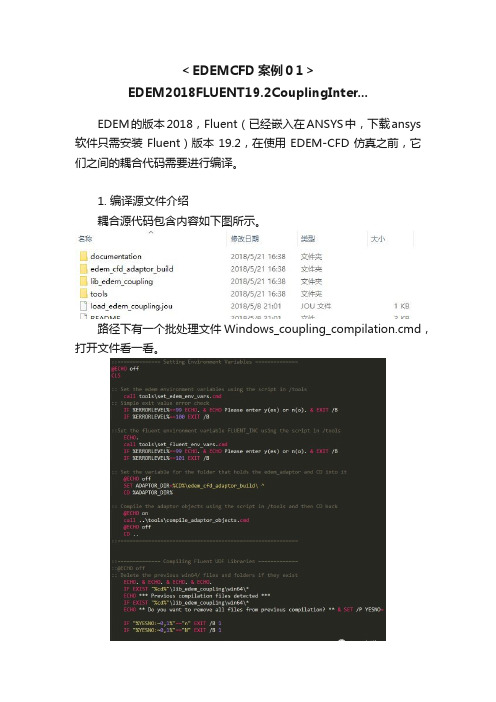
<EDEMCFD案例01>EDEM2018FLUENT19.2CouplingInter...EDEM的版本2018,Fluent(已经嵌入在ANSYS中,下载ansys 软件只需安装Fluent)版本19.2,在使用EDEM-CFD仿真之前,它们之间的耦合代码需要进行编译。
1. 编译源文件介绍耦合源代码包含内容如下图所示。
路径下有一个批处理文件Windows_coupling_compilation.cmd,打开文件看一看。
该批处理文件结构很简单,包含两部分内容:•设置环境变量。
主要通过tools文件夹下两个批处理文件set_edem_env_vars.cmd及tools\set_fluent_env_vars.cmd,其中前者设置EDEM环境变量,后者设置Fluent相关环境变量。
•调用tools文件夹下compile_lib_edem_coupling.py进行编译。
2. 环境变量设置2.1 EDEM环境变量用文本编辑器打开set_edem_env_vars.cmd,其中内容如下图所示。
其中第6行如下图所示,可以看到官方提供源代码中包含的EDEM版本包含2.6, 2.7, 2017.0, 2017.1, 2017.2,并不包含2018。
这里直接添加2018.2.2 Fluent环境变量用文本文件打开set_fluent_env_vars.cmd,该批处理文件用于设置Fluent相关的环境变量。
文件第6行输入Fluent版本,如下图所示,并无19.2版本。
直接添加Fluent19.2版本。
实际上可以直接通过环境变量来解决问题。
3. 编译代码•启动VS2015 x64本机工具命令提示符(安装了VS2015之后就有),x64 Native Tools Command Prompt。
•编译需要用到python指令,需要将python指令添加到path 下,可以自行下载python安装;ANSYS也提供了python的一个版本,我安装在D:\Program Files\ANSYS Inc\v192\commonfiles\CPython\2_7_13\winx64\Release\python 该路径下,根据安装的路径和版本不同,D:\Program Files、v192、2_7_13可能是不同的。
ANSYS Workbench LS-DYNA流固耦合方法应用

ANSYS Workbench LS-DYNA流固耦合方法应用贮液容器(含塑料瓶)广泛应用于化工、食品包装、储运等领域。
由于容器(含塑料瓶)在运输和使用过程中常常会因为跌落或碰撞冲击导致破损而造成损失和污染,因此,研究贮液容器(含塑料瓶)在跌落碰撞过程中的力学行为,对认识容器(含塑料瓶)跌落碰撞损伤机理,优化容器(含塑料瓶)结构,提高其安全性和使用价值意义重大。
.贮液容器的跌落是一个典型的流固耦合问题,可采用LS-DYNA的ALE算法(任意拉格朗日欧拉算法)进行模拟。
下面以一个封闭的装水水箱为例,介绍ANSYS Workbench LS-DYNA分析此类型跌落问题的方法和步骤:1.建立几何模型调用ANSYS Workbench中的LS-DYNA模块,如图1所示。
然后使用ANSYS的CAD工具DesignModeler建立几何模型,如图2所示。
图1 调用Workbench LS-DYNA 图2 DesignModeler中建立几何模型2.生成K文件双击进入“Model”后,对模型进行网格划分、边界条件设置、速度设置和分析设置,如图3所示。
设置完成后点击“solve”求解,生成K文件,如图4所示。
图3 调用Workbench LS-DYNA 图4 DesignModeler中建立几何模型3.编辑K文件通过Workbench LS-DYNA生成的K文件中关键字是不够完善的,并不能直接递交LS-DYNA求解器进行求解。
K文件中所欠缺的一些关键字,在流固耦合分析中是必不可少的,如空材料的定义、跟随坐标系的定义、空白域的定义以及状态方程的定义等。
3.1 重要关键字释义(1)LS-DYNA程序提供了运动的多物质ALE网格,可以方便地为多物质ALE算法定义跟随坐标系*ALE_REFERENCE_SYSTEM_NODE*ALE_REFERENCE_SYSTEM_GROUP(2)定义空材料和状态方程的关键字*MAT_NULL *EOS(3)初始化空白域的关键字*INITIAL_VOID_PART(4)结构和流体之间耦合的关键字*CONSTRAINED_LAGRANGE_IN_SOLID(5)单元算法定义(单点积分的单物质加空白材料)的关键字*SECTION_SOLID_ALE ELF0RM=12(6)在重力作用下产生下落的关键字*LOAD_BODY……3.2关键字编辑方法关键字的编辑或修改一般有两种方法,一种是直接在ls-prepost中对关键字进行编辑设置,如图5所示;另一种是在文本编辑器UltraEdit中对关键字进行编辑或修改,如图6所示。
- 1、下载文档前请自行甄别文档内容的完整性,平台不提供额外的编辑、内容补充、找答案等附加服务。
- 2、"仅部分预览"的文档,不可在线预览部分如存在完整性等问题,可反馈申请退款(可完整预览的文档不适用该条件!)。
- 3、如文档侵犯您的权益,请联系客服反馈,我们会尽快为您处理(人工客服工作时间:9:00-18:30)。
相关专题: 颗粒仿真 无微不至_EDEM软件
更多资料:/Home.html
出在其他条件一定的情况下,随着振幅和频率的增加,物料沿筛面后移的速度
增加,同时透筛效率增高,在振幅40mm时和频率6Hz时出现筛分损失;随着振动 方向角的增大,在25°到45°范围内,物料沿筛面后移的速度增加,在45°时达
到最大,超过45°之后,物料沿筛面后移的速度逐渐降低,而透筛效率在35°时
最高,超过35°,透筛效率逐渐降低。模拟结果与试验测量结果总体趋势基本 吻合,这表明了利用EDEM进行数值模拟的正确性和可行性。
EDEM与ANSYS Workbench耦合介绍及案例 展示专题资料集锦
更新时间:2014-12-22
以下是小编整理的一些有关EDEM与ANSYS Workbench耦合介绍及案例展示专
题资料,其中包括了有关EDEM的相关资讯以及相关的案例文档和视频资料。 有关文档的下载,可以到研发埠网站的专题模块,输入相应的专题名,搜索
EDEM V2.6.1新版本功能及案例展示.pdf
EDEM与ANSYS Workbench(视频)
聚焦EDEM: EDEM两相流高级网络培训【视频】
EDEM联合XFlow CFD仿真流体系统中的颗粒运动
颗粒筛分问题EDEM模拟算例
EDEM?模拟高压辊磨机(HPGR)粉碎过程
相关文献: 基于EDEM的振动筛分数值模拟与分析.pdf 为了寻找振动筛的最佳运动学参数(振幅、频率、振动方向角),达到提高透筛 效率并减少清选损失的目的,利用EDEM软件,对振动筛分过程进行数值模拟,得
离散元仿真软件EDEM联合仿真结构分析方法.pdf EDEM联合仿真概述,EDEM动力学模块应用方法与案例演示,EDEM-FEM应用方 法与案例演。<br> EDEM是一款基于离散元(DiscreteElement Method,简称DEM)的颗粒力学仿真软件,可以模拟散体物料加工处理过程中 颗粒体系的行为特征,协助设计人员对相关工艺及设备进行分析和优化。另 外,EDEM还可以与CFD、FEA、MBD软件联合仿真,进行颗粒-流体问题分析、 设备应力分析、多体动力学分析等。
离散元仿真软件EDEM用户大会报告.pdf
EDEM基础知识,已经使用EDEM软件仿真流程,和实验数据的对比,从而凸显 EDEM软件的优势。
离散元仿真软件EDEM应用探讨—散体物料储存和输送的相关研究.pdf
离散元仿真软件EDEM在散体物料储存和输送的相关研究。
离散元仿真软件EDEM在密集的介质旋流中的多相流CFD-DEM建模(EN).pdf 离散元仿真软件EDEM在密集的介质旋流中的多相流CFD-DEM建模。
离散元仿真软件EDEM概述(EN).pdf
离散元仿真软件EDEM概述。EDEM是一款基于离散元(DiscreteElement Method,简称DEM)的颗粒力学仿真软件,可以模拟散体物料加工处理过程中 颗粒体系的行为特征,协助设计人员对相关工艺及设备进行分析和优化。另 外,EDEM还可以与CFD、FEA、MBD软件联合仿真,进行颗粒-流体问题分析、 设备应力分析、多体动力学分析等。
基于高阶离散格式的CFD与DEM耦合方法及其应用.rar
流固耦合现象广泛存在于自然界和工业生产中,例如风沙流动、气力输送、 流化过程等。同样气吹式排种器也可以作为流固耦合的研究对象
基于EDEM_FLUENT耦合的气吹式排种器工作过程仿真分析.rar
以一种气吹式排种器和吉科豆种子为研究对象,将种子颗粒按离散相处理, 通过牛顿定律求解每个颗粒的运动,即离散元法(DEM);同时将气体按连续
离散元仿真软件EDEM仿真粒子结构和颗粒流体的交互(EN).pdf
离散元仿真软件EDEM仿真粒子结构和颗粒流体的交互。
离散元仿真软件EDEM在钢铁工业领域 的应用及探讨.pdf
EDEM简述,钢铁工业领域的散装物料,EDEM并行计算,展望与讨论. EDEM是一款基于离散元(DiscreteElement Method,简称DEM)的颗粒力学仿 真软件,可以模拟散体物料加工处理过程中颗粒体系的行为特征,协助设计 人员对相关工艺及设备进行分析和优化。另外,EDEM还可以与CFD、FEA、MBD 软件联合仿真,进行颗粒-流体问题分析、设备应力分析、多体动力学分析等 。
相处理
基于离散单元法气力输送的数值模拟研究.rar
采用气力输送将散料从一个地方输送到另一个地方是化工、冶金、农业加工 过程中最为常用的方法。这种散料输送方法对环境污染小、操作灵活、能够 全部自动化。
离散元仿真软件EDEM多相流CFD-DEM模型在密集的介质旋流中的使用(EN) D-DEM模型在密集的介质旋流中的使用。
到相应的专题便可以找到相应的文档,或是到研发埠网站的版块输入相应的文档名查找。
颗粒系统仿真分析软件EDEM 2.6版本发布 为了帮助客户使用EDEM更高效的进行仿真计算,英国DEM Solutions公司于近 期发布了EDEM新版本V2.6,该版本进行了40多项创新性改进,专门针对客户 需求而开发,提高了软件的实用性、可靠性、计算效率以及与其它CAE工具的 耦合能力。