图像处理_3D Photography Dataset(华盛顿大学3D相机标定数据库)
ERDASIMAGINE遥感图像处理教程
《ERDAS IMAGINE遥感图像处理教程》根据作者多年遥感应用研究和ERDAS IMAGINE软件应用经验编著而成,系统地介绍了ERDAS IMAGINE 9.3的软件功能及遥感图像处理方法。
全书分基础篇和扩展篇两部分,共25章。
基础篇涵盖了视窗操作、数据转换、几何校正、图像拼接、图像增强、图像解译、图像分类、子像元分类、矢量功能、雷达图像、虚拟GIS、空间建模、命令工具、批处理工具、图像库管理、专题制图等ERDAS IMAGINE Professional级的所有功能,以及扩展模块Subpixel、Vector、OrthoRadar、VirtualGIS等;扩展篇则主要针对ERDAS IMAGINE 9.3的新增扩展模块进行介绍,包括图像大气校正(ATCOR)、图像自动配准(AutoSync)、高级图像镶嵌(MosaicPro)、数字摄影测量(LPS)、三维立体分析(Stereo Analyst)、自动地形提取(Automatic Terrain Extraction)、面向对象信息提取(Objective)、智能变化检测(DeltaCue)、智能矢量化(Easytrace)、二次开发(EML)等十个扩展模块的功能。
《ERDAS IMAGINE遥感图像处理教程》将遥感图像处理的理论和方法与ERDAS IMAGINE软件功能融为一体,可以作为ERDAS IMAGINE软件用户的使用教程,对其他从事遥感技术应用研究的科技人员和高校师生也有参考价值。
基础篇第1章概述21.1 遥感技术基础21.1.1 遥感的基本概念21.1.2 遥感的主要特点21.1.3 遥感的常用分类31.1.4 遥感的物理基础31.2 ERDAS IMAGINE软件系统6 1.2.1 ERDAS IMAGINE概述6 1.2.2 ERDAS IMAGINE安装7 1.3 ERDAS IMAGINE图标面板11 1.3.1 菜单命令及其功能111.3.2 工具图标及其功能141.4 ERDAS IMAGINE功能体系14第2章视窗操作162.1 视窗功能概述162.1.1 视窗菜单功能172.1.2 视窗工具功能172.1.3 快捷菜单功能182.1.4 常用热键功能182.2 文件菜单操作192.2.1 图像显示操作202.2.2 图形显示操作222.3 实用菜单操作232.3.1 光标查询功能232.3.2 量测功能242.3.3 数据叠加显示252.3.4 文件信息操作272.3.5 三维图像操作292.4 显示菜单操作332.4.1 文件显示顺序332.4.2 显示比例操作332.4.3 显示变换操作342.5 AOI菜单操作342.5.1 打开AOI工具面板35 2.5.2 定义AOI显示特性35 2.5.3 定义AOI种子特征35 2.5.4 保存AOI数据层36 2.6 栅格菜单操作372.6.1 栅格工具面板功能37 2.6.2 图像对比度调整392.6.3 栅格属性编辑402.6.4 图像剖面工具432.7 矢量菜单操作452.7.1 矢量工具面板功能46 2.7.2 矢量文件生成与编辑472.7.3 改变矢量要素形状482.7.4 调整矢量要素特征482.7.5 编辑矢量属性数据492.7.6 定义要素编辑参数502.8 注记菜单操作502.8.1 创建注记文件512.8.2 设置注记要素类型522.8.3 放置注记要素522.8.4 注记要素属性编辑542.8.5 添加坐标格网55第3章数据输入/输出563.1 数据输入/输出概述563.2 二进制图像数据输入573.2.1 输入单波段数据573.2.2 组合多波段数据583.3 其他图像数据输入/输出59 3.3.1 HDF图像数据输入操作59 3.3.2 JPG图像数据输入/输出60 3.3.3 TIFF图像数据输入/输出61第4章数据预处理624.1 遥感图像处理概述62 4.1.1 遥感图像几何校正62 4.1.2 遥感图像裁剪与镶嵌63 4.1.3 数据预处理模块概述63 4.2 三维地形表面处理64 4.2.1 启动三维地形表面64 4.2.2 定义地形表面参数65 4.2.3 生成三维地形表面66 4.2.4 显示三维地形表面67 4.3 图像几何校正674.3.1 图像几何校正概述67 4.3.2 资源卫星图像校正70 4.3.3 遥感图像仿射变换76 4.3.4 航空图像正射校正78 4.4 图像裁剪处理814.4.1 图像规则裁剪814.4.2 图像不规则裁剪824.4.3 图像分块裁剪844.5 图像镶嵌处理844.5.1 图像镶嵌功能概述84 4.5.2 卫星图像镶嵌处理90 4.5.3 航空图像镶嵌处理934.6 图像投影变换954.6.1 启动投影变换954.6.2 投影变换操作964.7 其他预处理功能964.7.1 生成单值栅格图像964.7.2 重新计算图像高程974.7.3 数据发布与浏览准备97 4.7.4 产生或更新图像目录98 4.7.5 图像范围与金字塔计算99第5章图像解译1005.1 图像解译功能概述1005.1.1 图像空间增强1005.1.2 图像辐射增强1015.1.3 图像光谱增强1015.1.4 高光谱基本工具1025.1.5 高光谱高级工具1035.1.6 傅里叶变换1035.1.7 地形分析功能1045.1.8 地理信息系统分析104 5.1.9 实用分析功能1055.2 空间增强处理1065.2.1 卷积增强处理106 5.2.2 非定向边缘增强107 5.2.3 聚焦分析1085.2.4 纹理分析1095.2.5 自适应滤波1105.2.6 统计滤波1115.2.7 分辨率融合1115.2.8 改进IHS融合112 5.2.9 HPF图像融合114 5.2.10 小波变换融合115 5.2.11 删减法融合1165.2.12 Ehlers图像融合117 5.2.13 锐化增强处理118 5.3 辐射增强处理1205.3.1 查找表拉伸1205.3.2 直方图均衡化120 5.3.3 直方图匹配1215.3.4 亮度反转处理122 5.3.5 去霾处理1235.3.6 降噪处理1235.3.7 去条带处理1245.4 光谱增强处理1245.4.1 主成分变换1245.4.2 主成分逆变换1255.4.3 独立分量分析1265.4.4 去相关拉伸1275.4.5 缨帽变换1275.4.6 色彩变换1295.4.7 色彩逆变换1295.4.8 指数计算1305.4.9 自然色彩变换1315.4.10 ETM反射率变换131 5.4.11 光谱混合器1335.5 高光谱基本工具135 5.5.1 自动相对反射1355.5.2 自动对数残差1365.5.3 归一化处理1365.5.4 内部平均相对反射137 5.5.5 对数残差1375.5.6 数值调整1385.5.7 光谱均值1395.5.8 信噪比功能1395.5.9 像元均值1405.5.10 光谱剖面1415.5.11 光谱数据库1425.6 高光谱高级工具142 5.6.1 异常探测1425.6.2 目标探测1475.6.3 地物制图1495.6.4 光谱分析工程向导153 5.6.5 光谱分析工作站154 5.7 傅里叶变换1565.7.1 快速傅里叶变换156 5.7.2 傅里叶变换编辑器157 5.7.3 傅里叶图像编辑158 5.7.4 傅里叶逆变换1685.7.5 傅里叶显示变换169 5.7.6 周期噪声去除1695.7.7 同态滤波1705.8 地形分析1715.8.1 坡度分析1715.8.2 坡向分析1715.8.3 高程分带1725.8.4 地形阴影1735.8.5 彩色地势1735.8.6 地形校正1755.8.7 栅格等高线1755.8.8 点视域分析1765.8.9 路径视域分析181 5.8.10 三维浮雕1825.8.11 高程转换1835.9 地理信息系统分析184 5.9.1 邻域分析1845.9.2 周长计算1865.9.3 查找分析1865.9.4 指标分析1875.9.5 叠加分析1885.9.6 矩阵分析1895.9.7 归纳分析1905.9.8 区域特征1905.10 实用分析功能191 5.10.1 变化检测1915.10.2 函数分析1925.10.3 代数运算1925.10.4 色彩聚类1935.10.5 高级色彩聚类194 5.10.6 数值调整1955.10.7 图像掩膜1965.10.8 图像退化197 5.10.9 去除坏线197 5.10.10 投影变换198 5.10.11 聚合处理199 5.10.12 形态学计算199第6章图像分类202 6.1 图像分类简介202 6.1.1 非监督分类202 6.1.2 监督分类2036.1.3 专家系统分类206 6.2 非监督分类2086.2.1 获取初始分类209 6.2.2 调整分类结果210 6.3 监督分类2126.3.1 定义分类模板213 6.3.2 评价分类模板221 6.3.3 执行监督分类226 6.3.4 评价分类结果227 6.4 分类后处理2316.4.1 聚类统计2326.4.2 过滤分析2326.4.3 去除分析2336.4.4 分类重编码2336.5 专家分类器2346.5.1 知识工程师2356.5.2 变量编辑器2396.5.3 建立知识库2426.5.4 知识分类器248第7章子像元分类2517.1 子像元分类简介2517.1.1 子像元分类的基本特征251 7.1.2 子像元分类的基本原理252 7.1.3 子像元分类的应用领域253 7.1.4 子像元分类模块概述254 7.2 子像元分类方法2567.2.1 子像元分类流程2567.2.2 图像质量确认2587.2.3 图像预处理2597.2.4 自动环境校正2607.2.5 分类特征提取2637.2.6 分类特征组合2697.2.7 分类特征评价2717.2.8 感兴趣物质分类2747.2.9 分类后处理2767.3 子像元分类实例2777.3.1 图像预处理2777.3.2 自动环境校正2777.3.3 分类特征提取2787.3.4 感兴趣物质分类2797.3.5 查看验证文件2817.3.6 分类结果比较282第8章矢量功能2838.1 空间数据概述2838.1.1 矢量数据2838.1.2 栅格数据2848.1.3 矢量和栅格数据结构比较285 8.1.4 矢量数据和栅格数据转换286 8.2 矢量模块功能简介2898.3 矢量图层基本操作2898.3.1 显示矢量图层2898.3.2 改变矢量特性2908.3.3 改变矢量符号2918.4 要素选取与查询2988.4.1 查看选择要素属性2988.4.2 多种工具选择要素2998.4.3 判别函数选择要素3008.4.4 显示矢量图层信息3028.5 创建矢量图层3038.5.1 创建矢量图层的基本方法303 8.5.2 由ASCII文件创建点图层307 8.5.3 镶嵌多边形矢量图层3088.5.4 创建矢量图层子集3108.6 矢量图层编辑3118.6.1 编辑矢量图层的基本方法311 8.6.2 变换矢量图层3138.6.3 产生多边形Label点3148.7 建立拓扑关系3148.7.1 Build矢量图层3158.7.2 Clean矢量图层3158.8 矢量图层管理3168.8.1 重命名矢量图层3168.8.2 复制矢量图层3178.8.3 删除矢量图层3178.8.4 导出矢量图层3188.9 矢量与栅格转换3188.9.1 栅格转换矢量3188.9.2 矢量转换栅格3208.10 表格数据管理3228.10.1 INFO表管理3228.10.2 区域属性统计3288.10.3 属性转换为注记329 8.11 Shapefile文件操作331 8.11.1 重新计算高程3318.11.2 投影变换操作332第9章雷达图像处理3349.1 雷达图像处理基础334 9.1.1 雷达图像增强处理334 9.1.2 雷达图像几何校正336 9.1.3 干涉雷达DEM提取336 9.2 雷达图像模块概述337 9.3 基本雷达图像处理337 9.3.1 斑点噪声压缩3389.3.2 边缘增强处理3409.3.3 雷达图像增强3419.3.4 图像纹理分析3449.3.5 图像亮度调整3459.3.6 图像斜距调整3469.4 正射雷达图像校正3479.4.1 正射雷达图像校正概述347 9.4.2 地理编码SAR图像3489.4.3 正射校正SAR图像3529.4.4 GCP正射较正SAR图像355 9.4.5 比较OrthoRadar校正效果358 9.5 雷达像对DEM提取3599.5.1 雷达像对DEM提取概述359 9.5.2 雷达立体像对数据准备359 9.5.3 立体像对提取DEM工程360 9.6 干涉雷达DEM提取3699.6.1 干涉雷达DEM提取概述369 9.6.2 干涉雷达图像数据准备369 9.6.3 干涉雷达DEM提取工程370 9.6.4 DEM高程生成3759.7 干涉雷达变化检测3769.7.1 干涉雷达变化检测模块376 9.7.2 干涉雷达变化检测操作377第10章虚拟地理信息系统381 10.1 VirtualGIS概述38110.2 VirtualGIS视窗38210.2.1 启动VirtualGIS视窗382 10.2.2 VirtualGIS视窗功能382 10.3 VirtualGIS工程38510.3.1 创建VirtualGIS工程385 10.3.2 编辑VirtualGIS视景387 10.4 VirtualGIS分析39110.4.1 洪水淹没分析39110.4.2 矢量图形分析39410.4.3 叠加文字注记39610.4.4 叠加三维模型39810.4.5 模拟雾气分析40510.4.6 威胁性与通视性分析406 10.4.7 立体视景操作40910.4.8 叠加标识图像41010.4.9 模拟云层分析41210.5 VirtualGIS导航41410.5.1 设置导航模式41410.5.2 VirtualGIS漫游415 10.6 VirtualGIS飞行41610.6.1 定义飞行路线41710.6.2 编辑飞行路线41910.6.3 执行飞行操作42010.7 三维动画制作42010.7.1 三维飞行记录42110.7.2 三维动画工具42210.8 虚拟世界编辑器42210.8.1 虚拟世界编辑器简介422 10.8.2 创建一个虚拟世界425 10.8.3 虚拟世界的空间操作429 10.9 空间视域分析43110.9.1 视域分析数据准备431 10.9.2 生成多层视域数据432 10.9.3 虚拟世界视域分析434 10.10 设置VirtualGIS默认值436 10.10.1 默认值设置环境436 10.10.2 默认值设置选项436 10.10.3 保存默认值设置439第11章空间建模工具44011.1 空间建模工具概述44011.1.1 空间建模工具的组成440 11.1.2 图形模型的基本类型441 11.1.3 图形模型的创建过程44111.2 模型生成器功能组成442 11.2.1 模型生成器菜单命令442 11.2.2 模型生成器工具图标443 11.2.3 模型生成器工具面板444 11.3 空间建模操作过程444 11.3.1 创建图形模型44411.3.2 注释图形模型44711.3.3 生成文本程序44811.3.4 打印图形模型44911.4 条件操作函数应用450第12章图像命令工具453 12.1 图像信息管理技术453 12.1.1 图像金字塔45312.1.2 图像世界文件45312.2 图像命令工具概述454 12.3 图像命令功能操作455 12.3.1 改变栅格图像类型455 12.3.2 计算图像统计值456 12.3.3 图像金字塔操作457 12.3.4 图像地图模式操作458 12.3.5 图像地图投影操作45912.3.6 图像高程信息操作45912.3.7 图像文件常规操作461第13章批处理操作46213.1 批处理功能概述46213.2 批处理系统设置46213.3 批处理操作过程46313.3.1 单文件单命令批处理463 13.3.2 多文件单命令立即批处理465 13.3.3 多文件单命令随后批处理467 13.3.4 多文件多命令批处理469第14章图像库管理47314.1 图像库管理概述47314.2 图像库环境设置47314.3 图像库功能介绍47414.3.1 打开默认图像库47414.3.2 图像库管理功能47514.3.3 图像库图形查询476第15章地图编制47915.1 地图编制概述47915.1.1 地图编制工作流程479 15.1.2 地图编制模块概述479 15.2 地图编制操作过程48015.2.1 准备制图数据48015.2.2 创建制图文件48015.2.3 确定地图制图范围481 15.2.4 放置整饰要素48215.2.5 地图打印输出48915.3 制图文件路径编辑48915.4 系列地图编制工具49015.4.1 准备系列地图编辑文件490 15.4.2 启动系列地图编辑工具490 15.4.3 显示系列地图分幅信息491 15.4.4 系列地图输出编辑491 15.4.5 保存系列地图文件492 15.4.6 系列地图输出预览492 15.5 地图数据库工具492扩展篇第16章图像大气校正49616.1 大气校正模块概述49616.1.1 ATCOR模块主要特征49616.1.2 ATCOR模块功能组成497 16.2 太阳位置的计算49716.3 ATCOR2工作站49816.3.1 ATCOR2工程文件498 16.3.2 光谱分析模块50216.3.3 常数大气模块50716.3.4 增值产品模块51016.4 ATCOR3工作站51116.4.1 ATCOR3生成地形512 16.4.2 ATCOR3工程文件512 16.4.3 光谱分析模块51516.4.4 常数大气模块51516.4.5 增值产品模块516第17章图像自动配准51817.1 图像自动配准模块概述518 17.2 地理参考配准51917.2.1 准备图像数据51917.2.2 产生自动配准点52017.2.3 选择几何模型52317.2.4 定义投影类型52517.2.5 确定输出图像52617.3 图像边缘匹配52717.3.1 准备输入图像52717.3.2 产生自动匹配点52817.3.3 定义匹配策略52817.3.4 选择投影类型52917.3.5 确定输出图像52917.4 自动配准工程52917.4.1 保存自动配准工程文件529 17.4.2 打开自动配准工程文件530 17.5 自动配准工作站53017.5.1 自动配准工作站功能概述530 17.5.2 自动配准工作站应用流程535第18章高级图像镶嵌54318.1 高级图像镶嵌功能概述543 18.1.1 MosaicPro模块特点543 18.1.2 MosaicPro启动过程543 18.1.3 MosaicPro视窗功能544 18.2 高级图像镶嵌工作流程546 18.2.1 航空图像镶嵌54618.2.2 卫星图像镶嵌55318.2.3 图像匀光处理559第19章数字摄影测量56119.1 数字摄影测量基本原理561 19.1.1 数字摄影测量处理过程561 19.1.2 数字图像的内定向56219.1.3 图像核线数字相关56319.1.4 建立规则格网DEM 56319.1.5 图像正射校正处理56419.2 LPS工程管理器56619.2.1 LPS工程管理器功能概述566 19.2.2 LPS工程管理器视窗组成567 19.3 摄影图像摄影测量处理570 19.3.1 摄影图像处理流程57019.3.2 创建LPS工程文件57019.3.3 向LPS工程加载图像572 19.3.4 定义摄影相机几何模型573 19.3.5 定义地面控制点与检查点576 19.3.6 图像同名点自动量测583 19.3.7 执行航空三角测量58419.3.8 图像正射校正处理58719.4 数码图像摄影测量处理588 19.4.1 数码图像处理流程58919.4.2 创建LPS工程文件58919.4.3 向LPS工程加载图像59219.4.4 定义数码相机几何模型59319.4.5 自动量测图像同名点59519.4.6 执行航空三角测量59719.4.7 图像正射校正处理60019.5 扫描图像摄影测量处理60119.5.1 扫描图像处理流程60119.5.2 创建LPS工程文件60119.5.3 加载并定义第一幅图像60319.5.4 加载并定义第二幅图像61019.5.5 图像同名点自动量测61319.5.6 执行空间三角测量61419.5.7 图像正射校正处理616第20章三维立体分析61820.1 三维立体分析基本原理61820.1.1 基于立体像对的高程模型提取618 20.1.2 三维场景重建的实现方法619 20.2 三维立体分析模块概述62120.2.1 三维立体分析模块特点62220.2.2 三维立体分析模块功能62220.3 创建非定向数字立体模型62320.3.1 启动三维立体分析模块62320.3.2 加载三维立体分析图像62320.3.3 调整图像显示参数62520.3.4 保存三维立体模型627第21章自动地形提取62821.1 LPS自动地形提取概述62821.1.1 DTM及其自动提取方法62821.1.2 LPS自动地形提取功能62821.1.3 LPS自动地形提取过程62921.2 LPS自动地形提取操作63021.2.1 创建LPS工程文件63021.2.2 DTM提取参数设置63221.2.3 DTM提取选项设置63321.2.4 DTM自动提取和检查637第22章面向对象的信息提取63922.1 面向对象的信息提取简介63922.1.1 IMAGINE Objective框架设计639 22.1.2 IMAGINE Objective关键特征639 22.2 道路信息提取64022.2.1 道路信息提取模型640 22.2.2 道路信息提取过程640第23章智能变化检测64323.1 智能变化检测原理64323.1.1 图像预处理64323.1.2 变化检测方法64323.1.3 变化定量分析64823.2 智能变化检测应用特点649 23.2.1 智能变化检测技术特征649 23.2.2 智能变化检测工作特点650 23.3 智能变化检测应用操作650 23.3.1 智能变化检测向导模式651 23.3.2 智能变化检测图像显示653 23.3.3 智能变化检测场地检测656第24章智能矢量化65724.1 智能矢量化模块概述657 24.1.1 模块的关键特征65724.1.2 模块的局限性65724.2 智能矢量化模块应用658 24.2.1 模块操作快捷键65824.2.2 启动智能矢量化模块658 24.2.3 跟踪线状地物中心线659 24.2.4 跟踪面状地物边界线662 24.3 智能矢量化模块使用技巧663第25章二次开发工具66525.1 二次开发宏语言EML概述665 25.2 编写EML二次开发程序666 25.2.1 编写EML程序的过程666 25.2.2 执行EML程序的过程667 25.2.3 丰富EML程序的功能667 25.3 EML接口C程序开发包671参考文献674。
3D Photography翻译
3D Photography: Final project report
人体三维扫描
Sam Calabrese Aabhishek Gandhi Changyin Zhou
{smc2171, asg2160, cz2166}@
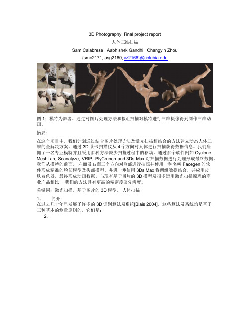
图1:模特为舞者。
通过对图片处理方法和按距扫描对模特进行三维摄像得到制作三维动画。
摘要:
在这个项目中,我们计划通过结合图片处理方法及激光扫描相结合的方法建立动态人体三
维的全解决方案。
通过3D莱卡扫描仪从4个方向对人体进行扫描获得数据信息。
我们雇
佣了一名专业模特并且采用多种方法减少扫描过程中的移动。
通过多个软件例如Cyclone, MeshLab, Scanalyze, VRIP, PlyCrunch and 3Ds Max对扫描数据进行处理形成最终数据。
我们从模特的前面,左面及右面三个方向对脸部进行拍照并使用一种名叫Facegen的软
件形成精准的脸部模型及头部模型。
并进一步使用3Ds Max将两组数据结合,并应用皮
肤着色器,最终形成动画数据。
与现有基于图片的3D模型及很多运用激光扫描原理的商
业产品相比,我们的方法具有更高的精密度及分辨度。
关键词:激光扫描,基于图片的3D模型,人体扫描
1、简介
在过去几十年里发展了许多的3D识别算法及系统[Blais 2004]。
这些算法及系统均是基于
三种基本的测量原则的,它们是:
2、。
CT图像重建算法与三维可视化技术
CT图像重建算法与三维可视化技术医疗行业一直是科技创新的重点,特别是在影像学领域,病人的诊断和治疗都需要借助高科技的医疗设备和技术。
计算机断层扫描技术(CT)是一项主流技术,它可以非常精确地显示人体内部的结构和器官。
CT扫描产生的图像数据是由计算机三维图像重建算法进行处理,然后再通过三维可视化技术呈现出来。
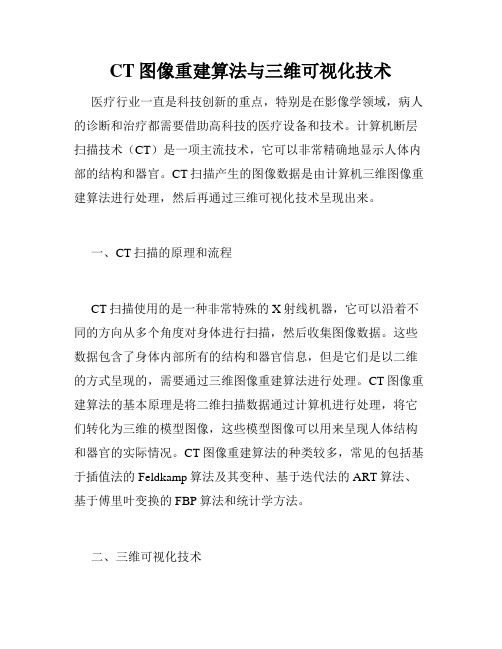
一、CT扫描的原理和流程CT扫描使用的是一种非常特殊的X射线机器,它可以沿着不同的方向从多个角度对身体进行扫描,然后收集图像数据。
这些数据包含了身体内部所有的结构和器官信息,但是它们是以二维的方式呈现的,需要通过三维图像重建算法进行处理。
CT图像重建算法的基本原理是将二维扫描数据通过计算机进行处理,将它们转化为三维的模型图像,这些模型图像可以用来呈现人体结构和器官的实际情况。
CT图像重建算法的种类较多,常见的包括基于插值法的Feldkamp算法及其变种、基于迭代法的ART算法、基于傅里叶变换的FBP算法和统计学方法。
二、三维可视化技术三维可视化技术一直是科技发展的焦点,它是将虚拟的三维物体以真实的方式呈现在屏幕上。
医学界常用的三维可视化技术主要包括直接体绘制,光线追踪、容积渲染、表面重建等多种方式。
直接体绘制是指在三维模型中直接绘制三维物体的方法。
光线追踪可以在保持真实性的同时,采用光线追踪技术来求解物体的表现方式,这种方法可以表现阴影、反射和折射等效应。
容积渲染则是将数据集表示为一组体元素(voxel),并利用光线传播和有效的颜色映射技术来生成具有透明度和色彩信息的图像。
表面重建是将容积表面转换为三角形网格的过程,从而实现三维模型的表面可视化。
三、可视化技术在医学诊断中的应用三维可视化技术在医疗领域应用广泛,它可以以更加直观的方式呈现病人身体的结构和器官情况,帮助医生诊断和制定治疗方案。
比如,医生可以使用三维可视化技术对肿瘤、脊柱和骨骼等进行预览,预测手术效果,规划术前准备,进行手术操作。
同时,在教育领域,三维可视化技术还可以对疾病的发展变化进行演示,帮助学生更好地理解医学知识,提高教育效果和学术思考能力。
NEWTON 7.0全植物成像系统说明书

NEWTON 7.0 - BIO Bioluminescence & Fluorescence Imgaging TEL: +1 (519) 914 5495 ***************** FAX: +1 (226) 884 5502 WHOLE PLANT IMAGINGSMART IMAGING SYSTEMFLUORESCENCE & BIOLUMINESCENCEAPPS STUDIO APPLICATION LIBRARYUltimate sensitivity with the widest f/0.70 lens apertureThe NEWTON 7.0 system combines high sensitivity with advanced plant imaging features and user-friendly time-saving operation.The NEWTON 7.0 proprietary optics have been specifically developed for macro imaging with high light collection capacity, incorporating a unique combination of high numerical aperture and long working distance. Bright fluorescence observation can be performed in a rapid scanning mode that shortens exposure times and minimizes specimen damage. Observation is thus possible even with slight body movement. The fast lens is also ideal for luminescence applications requiring longer exposure time.The NEWTON 7.0 includes our revolutionary Apps Studio approach to imaging. The Apps Studio is an innovative library of applications which contains more than 40 different protocols for a wide variety of targeted and easily activated fluorescent probes and reporters. The Apps Studio contains the excitation and the emission spectra of the main fluorophores used in modern molecular biology laboratory. It also suggestsThe advent of novel fluorescent probes has increased the demands on in-vivo fluorescence imaging systems to be able to deftly handle a variety of simultaneous signals. Our dual magnetron filter technology ensures transmission above 90% and very narrow band cutting - meaning improved spectral separation and increasedsensitivity. Our detection spectral range goes from 400to 900nm, making the NEWTON 7.0 ideal for GFP, YFP or IR applications. With the NEWTON 7.0 optical imaging system, you can image bioluminescent reporters like firefly luciferase and rapidly quantify the signal. The system allows you to visualize infections in whole plants and leaves, compare plant virology, regulate plants growth or observe the stress tolerance.A large number of dyes and stains can be used such as GFP, YFP, Pro-Q Emerald 300, Sypro-Ruby, FITC, DAPI,Alexa Fluor® 680, 700, 750, Cy® 3, 5, 5.5, DyeLight, IRDye® 800CW, VivoTrack 680, VivoTag 750…the best possible system configuration in terms of light source excitation, emission filter and sensitivity level. The Apps Studio ensures reproducibility and one click image acquisition for the best ease of use.The Newton 7.0 accomodates 8 excitation chanels in the visible RGB and NIR spectrum.. Signals can beoverlayed so that several reporters can be visualized simultaneously. Research on microbial infection of plants - BIK1 and FLS2interact with RbohD in N. benthamiana. The indicated constructs were transiently expressed in N. benthamiana,and luciferase complementation imaging assay was performed.Each individual light source delivers a precisely defined range of the spectrum. The very tight LED spectrum is additionally constrained with a very narrow excitation filter. This means less background in the images of your sample and a higher signal to noise ratio to detect the weakest signals. The LED Spectra Capsules can be easily changed, meaning that NEWTON 7.0 can be adapted simply as the requirements of your applicationsevolve.Cloned Plant screening: Arabidopsis thaliana seedlings transfected with luciferase (right) and nontransfected (left), 3min exposure after 1 mM luciferin was sprayed onto the leaves.The NEWTON’s protocoldriven image acquisition is as quick as it is intuitive: adjust your exposure, save, print or quantify.QUANTITATIVE IMAGINGPLANT MANIPULATION ROTATING STAGESUPERIOR QUANTITATIVERESULTSThe NEWTON 7.0 achieves the best signal to noise ratio for the lowest limits of detection. The system is extremely linear over its wide dynamics and can easily detect large intensity difference between bright and faint signals before reaching saturation. The broad linear dynamic range enables relative quantification of target proteins with confidence.Sensitivity is a key feature to detect a bioluminescence orfluorescence signal. Broad linear dynamic range is necessary to compare weak and strong signals in the same image.MULTISPECTRALIMAGINGCUSTOM MADE V.070 LENSNARROW BANDPASSFILTERSUltimate linearity for precise protein quantification over the full dynamic range.Ultra-low noise imaging thanks to a dualcamera amplifier architecture.NEWTON 7.0 Software - 3D Dynamic ScanThe NEWTON 7.0 BIO has been specially designed to handle plants with minimum manipulation. Simply position your pot on the dedicated tray, the stage can be inclined by 15° on the X/Y axis to visualize the plants from different angles and is easily controlled from the software interface, avoiding time consuming manipulation. The rotating stage is also motorized on the Z-axis to get closer to the CCD camera depending on your sample size, giving the possibility to image whole plants, leaves and seedlings with an enhanced sensitivity and image resolution.FUSION custom made lens for enhanced sensitivity and sharpness.Height Adjustable Plant StageTime to get the image is drastically reduced and precious antibody can be saved.Various imaging modes are available from automatic, manual, or time-lapse imaging program. Benefit from our 3D Dynamic Scan technology and observe the different signal intensities in a live 3D video reconstruction. The unique color imaging mode helps you acquire a quick snapshot of your plants with a true color representation,making the documentation faster!When a whole plant is being imaged, it could be difficult to focus on a specific part of the plant. With the NEWTON 7.0 BIO’s new generation of CCD camera, simply click on the leaf of interest for an immediate focusing with no manual adjustment.NEWTON 7.0 BIOVersatile ApplicationsPerformance• Comparative Plant Virology • Genetic Regulation • Infection Monitoring • Regulation of Plant Growth • Stress Tolerance• Proprietary V.070 lens with f0.70 aperture • 1” scientific grade CCD camera • Bioluminescence detection • Fluorescence detectionNEWTON 7.0 BIOLuciferase Expression GFP ExpressionChlorophyll Phosphorescence NIR IlluminationIntuitive user interfaceOne click to get the imageAuto-exposure and automatic illumination control Easy to cleanEase of UseWide DetectionMonitor the growth of a plant overtime thanks to the Daylight and Nightlight simulation modes. The system allows you to collect and compare data throughout the growth of plants.3 days 7 days 14 days 21 days 28 days 37 days 43 days50 daysSOFTWAREILLUMINATIONPERFORMANCENEWTON 7.0 BIOCAMERA & OPTICSHARDWARE CAPABILITIESIntelligent Darkroom concept Fully-automatic system •Motorized Optical Lens •Z-axis Motorized Camera •15° Tilting sample stageDual White-Light LED Panels 8 excitation channels:440nm - 480nm - 540nm - 580nm 640nm - 680nm - 740nm - 780nm 11-Position Motorized Filter Wheel 8 Narrow Bandpass Emission Filters: 500nm - 550nm - 600nm - 650nm 700nm - 750nm - 800nm - 850nmBioluminescence, Chemiluminescence & Fluorescence detectionScientific grade 16-bit CCD camera Grade 0, 400-900nm / 4.8 O.D.-90°C delta Coolingf/0.70 motorized lens aperture Image resolution: 10 megapixels Native resolution: 2160x2160Peak Quantum Efficiency: 80%FOV mininum: 6x6cm (macro imaging) FOV maximum: 20x20cm (whole plant)Bioluminescence detection : femtogram level Fluorescence detection : picogram levelAutomatic, Manual & Serial Acquisition modes Exposure time minimum: 40 milliseconds Exposure time maximum: 2 hours 3D live Dynamic ScanImage Editing and Image AnalysisincludedChemiluminescence and fluorescence on Western, Northern or Southern blot.eGFP transfected rice grainsexcitation 480nm and emission filter F-565,exposure time 0.8 sec.GFP expressionGFP-transfected (right) and Control (left) tobacco leaves, Epiexcitation 480nm and emission filter F-565,exposure time 2sec.Plant VirologyAgroinfiltration in Nicothiana Benthamania 16c, observed under blue excitation (480nm with F-565) to localize the GFP expressionCHINAVilber China Room 127 Building A N° 111 Yuquangying Fengtai District – Beijing ChinaPhone:+86136****1545**************GERMANYVilber L Deutschland GmbH Wielandstrasse 2D-88436 Eberhardzell DeutschlandPhone : + 49 (0) 7355 931 380**************HEADQUARTERS VilberZAC de Lamirault CollegienF-77601 Marne-la-Vallee cedex 3FrancePhone : + 33 (0) 1 60 06 07 71 ***************Disclaimer: Vilber’s NEWTON 7.0 Imager may be used in a wide range of imaging applications for research use only, including in vivo and in-vitro imaging in plants. No license under any third-party patent is conveyed with the purchase or transfer of this product. No right under any other patent claim, no right to perform any patented method, and no right to perform commercial services of any kind,including without limitation, reporting the results of purchaser’s activities for a fee or other commercial consideration, is conveyed expressly, by implication, or by estoppel. Therefore, users of the NEWTON 7.0 should seek legal advice to determine whether they require a license under one or more of the exiting patents in their country. This system is not intended for sale or transfer in the United States and Canada.TEL: +1 (519) 914 5495*****************FAX: +1 (226) 884 5502。
深度学习的多视角三维重建技术综述

深度学习的多视角三维重建技术综述目录一、内容概览 (2)1.1 背景与意义 (2)1.2 国内外研究现状 (3)1.3 研究内容与方法 (5)二、基于单目图像的三维重建技术 (6)2.1 基于特征匹配的三维重建 (7)2.1.1 SIFT与SURF算法 (8)2.1.2 PCA与LDA算法 (10)2.2 基于多视图立体视觉的三维重建 (11)2.3 基于深度学习的三维重建 (12)2.3.1 立体卷积网络 (14)2.3.2 多视图几何网络 (15)三、基于双目图像的三维重建技术 (17)3.1 双目立体视觉原理 (19)3.2 基于特征匹配的双目三维重建 (20)3.3 基于深度学习的双目三维重建 (21)3.3.1 双目卷积网络 (22)3.3.2 GANbased双目三维重建 (23)四、基于多视角图像的三维重建技术 (25)4.1 多视角几何关系 (26)4.2 基于特征匹配的多视角三维重建 (27)4.2.1 ORB特征在多视角场景中的应用 (28)4.2.2 ALOHA算法在多视角场景中的应用 (29)4.3 基于深度学习的多视角三维重建 (30)4.3.1 三维卷积网络(3DCNN)在多视角场景中的应用 (32)4.3.2 注意力机制在多视角场景中的应用 (33)五、三维重建技术在深度学习中的应用 (35)5.1 三维形状描述与识别 (36)5.2 三维物体检测与跟踪 (37)5.3 三维场景理解与渲染 (39)六、结论与展望 (40)6.1 研究成果总结 (41)6.2 现有方法的局限性 (42)6.3 未来发展方向与挑战 (44)一、内容概览多视角数据采集与处理:分析多视角三维重建的关键技术,如相机标定、图像配准、点云配准等,以及如何利用深度学习方法提高数据采集和处理的效率。
深度学习模型与算法:详细介绍深度学习在多视角三维重建中的应用,包括卷积神经网络(CNN)、循环神经网络(RNN)、生成对抗网络(GAN)等,以及这些模型在多视角三维重建任务中的优势和局限性。
计算机视觉技术中的三维重建方法与工具推荐

计算机视觉技术中的三维重建方法与工具推荐计算机视觉技术已经逐渐成为科学研究和工业应用中的重要工具。
在计算机视觉领域中,三维重建是一个重要的任务,它可以从一系列的二维图像或视频中恢复出场景的三维形状和纹理信息,为许多领域提供了强大的分析和设计能力。
本文将介绍几种常见的三维重建方法,并推荐一些常用的工具。
一、三维重建方法1. 隐式体素方法隐式体素方法是一种利用体素(体积像素)来表示和重建三维几何结构的方法。
该方法通常使用点云数据或体积数据作为输入,将对象建模为精细的体素网格,并从中提取几何信息。
常用的隐式体素方法有薄片轮廓隐式体素(TSDF)、体素边界网格(Voxel Boundary Grid)等。
这些方法虽然能够实现较高精度的三维重建,但由于体素表示的计算量较大,对计算资源的要求较高。
2. 稠密点云重建方法稠密点云重建方法使用从图像中提取的稀疏点云作为输入,通过使用匹配、滤波和插值等技术,将稀疏点云扩展为稠密点云。
该方法中常用的算法有基于多视图几何的方法和基于结构光的方法。
基于多视图几何的方法利用多个视角的图像进行几何重建,常用的算法包括光束法、三角测量法和基于匹配的方法。
而基于结构光的方法则是通过投射结构光或使用红外深度传感器捕捉场景中光的反射来获取场景的三维信息,常用的工具有Microsoft Kinect、Intel RealSense等。
3. 深度学习方法深度学习方法在计算机视觉领域中得到了广泛的应用。
在三维重建领域,深度学习方法可以通过训练神经网络来提取图像中的特征,并推断出场景的三维信息。
常用的深度学习方法包括卷积神经网络(CNN)和生成对抗网络(GAN)。
CNN 可以通过图像识别和分割来获取场景的二维特征,然后通过几何推理方法将其转化为三维信息。
GAN可以通过自适应学习生成具有真实感的三维模型。
这些方法在三维重建中取得了较好的效果,但对于数据量的要求较高,需要较大规模的训练数据集。
微软UltraMap 3.0:高级空中图像处理系统说明书
Ortho GenerationEssentials Dense MatchingAerial TriangulationRadiometryHighly advanced photogrammetric workflow system for UltraCam imagesMicrosoft UltraMap is a state-of-the-art, end-to-end, completephotogrammetric workflow system that provides highly automatedprocessing capabilities to allow organizations to rapidly generatequality data products from an UltraCam flight. UltraMap is designedto process huge amount of UltraCam data in the shortest possibletime with the highest degree of automatization, supported by guided manual interaction, quality control tools and powerful visualization. With version 3, UltraMap continues its innovation trend that has already delivered groundbreaking features such as monolithic stitching and automatic project-based color balancing for homogeneous image block color correction, but now also provides revolutionary, automated 3D data generation and ortho image processing features.UltraMap v3 now includes:• High-density 3D point cloud generation, with a point density of several hundred points per square meter, derived from an UltraCam photo mission• Highly accurate and detailed digital surface model (DSM) generation• Filtering of a DSM into a digital terrain model (DTM)• Generation of DSMOrtho (orthomosaic based on an automatically generated DSM) and DTMOrtho (traditional ortho mosaic) images UltraMap v3 delivers exceptional quality DSMOrthos and DTMOrthos athigh accuracies and without any manual interaction, since the UltraMapv3 ortho mosaicking approach takes into account all available inputs(i.e. a DSM and the automatically generated DTM). UltraMap v3 is able to generate seamlines at desired paths; remaining seamline editing for challenging regions is made using UltraMap’s DragonFly technology, a responsive visualization engine that allows users to conduct quality control on large image blocks in a quick and smooth fashion.UltraMap v3 is the first fully integrated and interactive photogrammetric workflow solution to provide premium UltraCam data processing from ingest of raw data to delivery of point clouds, DSMs and ortho imagery.ModulesUltraMap/Essentials | The UltraMap/Essentials module is responsible for converting the raw images taken by the UltraCam intostandard file formats that can be used by further processing steps in UltraMap and/or third party software systems. The UltraMap/Essentials module is divided into two processing steps:UltraMap/RawDataCenter | the UltraMap/RawDataCenter step is responsible for processing the UltraCamimagery from level-0 to level-2. By exploiting the distributed UltraMap Framework, processing tasks can be handled inparallel.UltraMap/Radiometry | the UltraMap/Radiometry step is responsible for defining the final color of thelevel-2 data. It also provides model-based radiometric correction to compensate for or remove hotspots, atmosphericeffects and haze, exploiting Dragonfly technology for image interaction and visualization of large image blocks.UltraMap/AT | the Aerial triangulation (AT) module provides an interactive workflow while calculating image correspondences in order to generate a precise exterior orientation for an entire image block by means of a least-squares bundle adjustment.UltraMap/DenseMatcher | the UltraMap/DenseMatcher module creates high-density point clouds and DSMs and DTMs from level-2 images, extrapolating precise exterior orientation data to generate per-pixel height values. The 3D point cloud and the DSM data can be exported in standard file formats for further 3rd party processing.UltraMap/OrthoPipeline | the UltraMap/OrthoPipeline module generates the final ortho mosaic from all available inputs such as level-2 imagery, AT results, radiometric settings, and the DSM/DTM. Two different ortho images can be generated:DSMOrthos and DTMOrthos.UltraMap/EssentialsThe UltraMap/RawDataCenter step of the UltraMap/Essentials module is responsible for downloading and processing of UltraCamimages from level-0 to level-2, including:• Geometrical corrections• Monolithic stitching• Radiometric corrections• Generation of the UltraMap project fileGeometrical corrections: UltraCam images are captured during aerial acquisition and stored in the RawData Format. Each shot position contains a number of sub-images. Each sub image corresponds to one single CCD sensor array and needs to be processed and converted by means of image stitching. This stitching process makes use of the overlapping footprint areas of the CCD sensor arrays. A larger number of points of interest are automatically detected and corresponding positions are computed by means of image correlation. The quality of this correlation process is at a 1/20 of a pixel magnitude, given that the image content of the analyzed region is very similar (no differences in the image content caused from perspective foreshortening and same lighting condition).Furthermore the Laboratory Calibration plays a significant role in this process and allows estimation of point positions to avoid mismatch and larger search areas. Metadata information, such as temperature readings, is included in order to describe the conditions of the camera for a distinct position at the moment of image capture. The image geometry is computed based on the stitching process (including panchromatic overlaps and color band information [cf. Monolithic Stitching]).The result of this process is the so-called level-2 image. It contains the high-resolution panchromatic image at the 16-bit per pixel data range and the 4-band multispectral image at 16-bit per band data format. The images are geometrically corrected and multispectral data are co-registered to the panchromatic image. It is worth noting that radiometric corrections are also applied to level-2 images based on the laboratory calibration (cf. radiometric corrections). As level-2 images are stored at 16-bit per band the radiometric domain is a linear domain without any logarithmic modification. Thus, one may call the level-2 image the “Digital transparency”.Stitching results are well documented by UltraMap. Thus one may study details of the level-2 processing and the stitching (left) or enjoy thecomprehensive overview with color-coded image frames (right).Monolithic stitching: The monolithic stitching generates one full frame PAN image out of the nine PAN sub-images taken by the camera. It uses information from the overlap between the nine sub-images as well as information from the full frame color cones to collect the tie points used for the stitching. This leads to a set of strong tie points between the sub-images even under critical conditions, such as images containing water bodies or images with unstructured terrain, such as sand desert. As a result, the full PAN frame of an UltraCam has a very robust and high accuracy literally as if it were collected by one large CCD through one lens. However the use of multiple smaller CCDs has significant benefits such as much higher image dynamic compared to single large CCDs. So, the monolithic stitching of UltraMap enables combining the benefits of image quality of smaller CCDs with the accuracy of large CCDs by avoiding the disadvantages of the latter. The overlap areas of CCD footprints and the resulting point distribution can be seen below. Stitching between panchromatic image areas allow collection of a large number of points at distinguished areas (left) and full frame distribution based on the color channel (right).Radiometric corrections: The radiometric correction is based on the radiometric parameters of the camera which are estimated during the Laboratory Calibration procedure. The parameters contain all information about the lenses, mechanical shutters and CCD detector arrays.Thus, the radiometric behavior of the camera is already known at a distinct quality level and can be adopted during the processing from raw images (level-0) to level-2. For this data, different F-stop settings are considered and the resulting vignetting masks are made available to the process.In a second step, the results from the radiometric analysis of CCD overlap areas is used to fine-tune the radiometric correction and remove any visible difference from adjacent image areas. Again the full frame color band contributes to this procedure and thus the monolithic stitching procedure also has an important benefit to the radiometric correction.A Vignetting Mask (left) and a shutter control diagram (right) are shown below as results from the radiometric laboratory calibration procedure.UltraMap Project File: This file is generated fully automatically during the first step of the processing. The file contains all important data and metadata of the distinct aerial project such as image file names, directory structure, camera parameters and initial exterior orientation data, as well as results from the ongoing processing. The UltraMap Project File has the extension .dfp and contains the basic information to allow any further automated processing of the entire photo mission. Below the Project File (e.g. UCEf80.dfp) can be recognized directly within the selected project folder listing.The Radiometry step of the UltraMap/Essentials module is responsible for defining the final color of the level-2 input data and togenerate level-3 output data. The step is fully automated and provides a rich feature set to adjust the color appearance of single images as well as the appearance of a whole block. However, deep manual interaction is possible to fine-tune the results to specific needs.Examples of the feature set are:• Automated, model-based radiometric correction to compensate for or remove hotspots and/or atmospheric effects such as haze• Project based color balancing (PBCB) for automated color correction of whole blocks. Effects such as different exposures, different illumination conditions and different flying time are corrected automatically• Smooth visualization and interaction of small and large blocks by the Dragonfly technology• Easy and intuitive user interface based on modern GUI technology and instant feedback• Full support of 16-bit workflow guarantees lossless computation of images• Various output formats for level-3 such as TIFF, 16bit TIFF, JPEG, single band, 3 band or 4 bandThe UltraMap/Essentials module is supported by the Dragonfly technology for the visualization and by the framework for distributed processing. This enables UltraMap to scale depending on throughput needs and IT infrastructure. Features such as distributed parallel processing (multi-core processing) with automated load balancing optimize throughput in heterogeneous networks without requiring any user interaction. The framework enables parallel processing on single computers as well as on small, medium and large multi-core systems.UltraMap/ATUltraMap/AT is the aerial triangulation module of UltraMap, optimized for UltraCam to deliver utmost quality. It provides an interactive workflow while calculating image correspondence to generate a precise exterior orientation for an entire image block. UltraMap/AT also focuses on a high degree of intelligent automatization. Wherever interaction is required, UltraMap/AT is designed to keep this interaction at a minimum, make it efficient and provides significant guidance for the interaction, such as the manual guided tie point improvement in the rare case that the automated tie-point collection did not provide the best possible results.Features of UltraMap/AT are:• Drag & Drop of GCPs• Uses in-flight GPS information for initial orientation• Single and multi-projection for ground control points• Initialization of project-based color balancing• Robust and automated tie point collection:• Guided manual point measurement (control points and tie points)• Auto-completion for manual point measurement• High accuracy due to a combination of feature-based and least-squares image matching• Sophisticated image-based tie point thinning for optimal coverage • Integrated photogrammetric bundle adjustment • Support for GPS/IMU data as a constraint for the bundle adjustment • Graphical overlays for AT results • Blunder detection, data snooping • Sub-block support • Visualized AT Report • Full support for all UltraCam cameras • Full support of 16-bit workflow • Supports scalable processing environments • Smooth visualization and interaction of small and large blocks by the Dragonfly technology• Easy and intuitive user interface•Full support of 16-bit workflowUltraMap/DenseMatcherA significant change in photogrammetry has been achieved by Multi-Ray Photogrammetry which became possible with the advent of the digital camera, such as the UltraCam, and a fully digital workflow by software systems such as UltraMap. This allows for significantly increased forward overlap as well as the ability to collect more images but virtually without increasing acquisition costs. However, Multi-Ray Photogrammetry as a first step is not a new technology; it is a specific flight pattern with a very high forward overlap (80%, even 90%) and an increased sidelap (up to 60%). The result is a highly redundant dataset that allows automated “dense matching” to generate high resolution, highly accurate point clouds from the imagery by matching the pixels of the overlapping images automatically.The UltraMap/DenseMatcher automatically generates point clouds from a set of overlapping UltraCam images. This is done by “pixel based matching” between all image pairs available for a given location on the ground. The precise exterior orientation is extrapolated and generates a height value (z-value) for a given pixel (for a given x, y, location). The redundancy of the image data set leads to multiple observations of z-values for a given location which will then be fused into one precise 3D measurement using sophisticated fusion algorithms. The remarkably high point density of the point cloud is typically of several hundred points per square meter.The achievable height accuracy of the point cloud is usually better than the GSD of the underlying images, thus a 10cm imagery leads to <10cm height accuracy of the resulting point cloud. This detailed and precise point cloud is used to generate a digital surface model (DSM). Thanks tothe high point density, this DSM has remarkably sharp edges and a very high level of detail.The next step after the DSM generation is the processing of a DTM. The DTM is processed out of the DSM using a hierarchical algorithm developed by Microsoft.Outputs of the UltraMap/DenseMatcher are:• considerably dense point clouds• Digital surface model (DSM)All outputs are available in standard formats for easy ingest into third party software systems. The digital terrain model (DTM) is currently onlybeing used internally in the UltraMap/OrthoPipeline for DTMOrtho image processing.UltraMap/OrthoPipelineMicrosoft UltraMap v3 introduces a fully automated processing pipeline for DSMOrtho and DTMOrtho generation.The DSMOrtho image is an ortho image which has been generated by rectifying the image, using the automatically generatedDSM. This leads to a special ortho image with no perspective view and no leaning objects, which has significant benefits in someapplications. Due to the consistent workflow, the DSMOrthos generated by UltraCam and UltraMap are of remarkably high-quality with very sharp edges, very detailed structures such as roof structures, and very little artifacts. That is because the dataset (DSM and images) comes from the same flight and no time difference has caused any changes on ground which could result in artifacts. Another reason for the high quality is theextremely sharp and precise DSM that has been processed from the point cloud, thanks to the high point density of the point cloud.The DTMOrtho is the traditional ortho image, processed by rectifying the images with a DTM that has also been generated automatically by the UltraMap/DenseMatcher. The seam lines have been generated automatically using information from the image content as well as from the heightfield. Manual editing tools support seamline optimization.RGB-DSMOrtho CIR-DSMOrthoThe UltraMap/OrthoPipeline consists of several steps which are performed in a sequence:Ortho rectification: the first step in the UltraMap/OrthoPipeline is called ortho rectification which re-projects the input images on a defined proxy geometry such as the DSM or the DTM. Depending on the type of the geometry used for the rectification, the result will be either a DSMOrtho or a DTMOrtho image.Seamline generation: after the ortho rectification process, the next step is the seamline computation between the rectified images. Seamscorrespond to transitions from an input image to the adjacent one.Ortho compositing: Once the initial ortho process is done, the software offers automated functionality to blend image content together in order to create a visually appealing result. All image bands (RGB and Near Infrared) are processed simultaneously in a consistent way.Processing EnvironmentThe UltraMap v3 processing pipeline is a highly scalable processing system that adapts flexibly to the IT environment.Key features and requirements are:• Use of mid-to-high-end standard Windows PCs is possible, allowing the use of existing infrastructure• Distributed processing in heterogeneous networks with automated load balancing ensure optimal usage of resources• Time guided machine allows to use of dedicated machines at dedicated time slots (e.g. using a workstation for UltraMap processing during night time).• Licensing scheme allows a wide spectrum of throughput needs. UltraMap can literally be executed on a laptop as well as on a processing system consisting of tens, or dozens or even hundreds of CPU cores and, as an option, additional GPU cores• Licensing scheme supports parallel setup of small field processing hubs (e.g. for immediate on-site quality checks after a flight) as well as setup of small, medium and large processing centers• GPU nodes deliver high-speed ups as the dense matching is ideal for a SIMD architecture such as graphics cards. Usage of CPU versus GPU can be configured to balance throughput• New V3 machines (resource intensive machines) provide high performance—an entire machine can be used to work on one task at a time. V3 machines can either be configured as CPU only or as GPU-enabled nodes.An UltraMap processing system usually consists of one or several front-end machines that are used to interact with the data and are not designed for processing. In addition, one or multiple processing machines are connected to the front end machine(s) and the data server(s). The processing machines handle data processing and may consist of multiple CPU and/or GPU nodes. The servers host the input, intermediate and final data. A very important part of the processing environment is the network required to transfer the data efficiently between front end, processing machines and servers.RGB-DTMOrtho CIR-DTMOrtho|*********************。
3d相机阈值 -回复
3d相机阈值-回复3D相机阈值(3D Camera Threshold)是指在3D相机应用中,为了准确地获取3D图像信息而设置的一个阈值。
本文将逐步探讨3D相机阈值的概念、作用、应用和调整方法。
第一步:概念解释3D相机阈值是指在3D相机应用中,为了准确地获取3D图像信息而设定的一个临界值。
这一阈值用于决定光线的强弱,进而判断目标物体的深度信息。
通过设定合适的阈值,可以有效地提高3D相机的测距精度和空间感知能力,从而满足不同应用场景下的需求。
第二步:作用说明3D相机阈值在图像处理中起到关键作用。
它通过对图像中的像素亮度进行分析和处理,能够准确地识别目标物体与其周围环境的差异,并生成深度图像。
通过深度图像的获取,相机可以实现对目标物体的测距、三维重建等功能。
因此,合适的阈值设定对于3D相机的性能和应用具有至关重要的影响。
第三步:应用领域3D相机阈值在许多领域得到广泛应用。
例如,它在机器人导航与感知中用于环境地图的构建和障碍物的识别;在电子商务中用于虚拟试衣和人脸识别技术;在自动驾驶中用于实时感知周围环境和距离测量等。
不同的应用场景对于阈值的要求各不相同,因此阈值的设定需要根据具体情况进行调整。
第四步:调整方法在实际应用中,调整3D相机阈值需要综合考虑多个因素。
以下是一些建议的调整方法:1. 确定目标物体的特征:根据目标物体的亮度、形状和颜色等特征,调整阈值来提取目标物体的深度信息。
不同物体的特征差异较大,因此可以根据目标物体的特点来设定合适的阈值。
2. 考虑光照条件:光照条件的变化会对3D相机的图像质量产生影响。
在强光、低光或背景光影响下,阈值的设定需要做出相应的调整,以获得清晰的深度图像。
3. 迭代调整:通过不断观察分析和实验调整,根据实际效果进行反馈,迭代地调整阈值。
这个过程需要耐心和经验,并且可能需要多次尝试才能得到满意的结果。
4. 结合其他算法:在一些复杂的场景中,单独依靠阈值可能无法获得准确的深度图像。
数字图像修复的DI灢StyleGANv2模型
第38卷第6期2023年12月安 徽 工 程 大 学 学 报J o u r n a l o fA n h u i P o l y t e c h n i cU n i v e r s i t y V o l .38N o .6D e c .2023文章编号:1672-2477(2023)06-0084-08收稿日期:2022-12-16基金项目:安徽省高校自然科学基金资助项目(K J 2020A 0367)作者简介:王 坤(1999-),男,安徽池州人,硕士研究生㊂通信作者:张 玥(1972-),女,安徽芜湖人,教授,博士㊂数字图像修复的D I -S t yl e G A N v 2模型王 坤,张 玥*(安徽工程大学数理与金融学院,安徽芜湖 241000)摘要:当数字图像存在大面积缺失或者缺失部分纹理结构时,传统图像增强技术无法从图像有限的信息中还原出更多所需的信息,增强性能有限㊂为此,本文提出了一种将解码信息与S t y l e G A N v 2相融合的深度学习图像修复方法 D I -S t y l e G A N v 2㊂首先由U -n e t 模块生成包含图像主信息的隐编码以及次信息的解码信号,随后利用S t y l e G A N v 2模块引入图像生成先验,在图像生成的过程中不但使用隐编码主信息,并且整合了包含图像次信息的解码信号,从而实现了修复结果的语义增强㊂在F F HQ 和C e l e b A 数据库上的实验结果验证了所提方法的有效性㊂关 键 词:图像修复;解码信号;生成对抗神经网络;U -n e t ;S t y l e G A N v 2中图分类号:O 29 文献标志码:A 数字图像是现代图像信号最常用的格式,但往往在采集㊁传输㊁储存等过程中,由于噪声干扰㊁有损压缩等因素的影响而发生退化㊂数字图像修复是利用已退化图像中存在的信息重建高质量图像的过程,可以应用于生物医学影像高清化㊁史物影像资料修复㊁军事科学等领域㊂研究数字图像修复模型具有重要的现实意义和商业价值㊂传统的数字图像修复技术多依据图像像素间的相关性和内容相似性进行推测修复㊂在纹理合成方向上,C r i m i n i s i 等[1]提出一种基于图像块复制粘贴的修补方法,该方法采用基于图像块的采样对缺失部分的纹理结构进行信息的填充㊂在结构相似性度研究上,T e l e a [2]提出基于插值的F MM 算法(F a s tM a r c -h i n g M e t h o d );B e r t a l m i o 等[3]提出基于N a v i e r -S t o k e s 方程和流体力学的图像视频修复模型(N a v i e r -S t o k e s ,F l u i dD y n a m i c s ,a n d I m a g e a n dV i d e o I n p a i n t i n g )㊂这些方法缺乏对图像内容和结构的理解,一旦现实中待修复图像的纹理信息受限,修复结果就容易产生上下文内容缺失语义;同时它们需要手动制作同高㊁宽的显示待修复区域的掩码图像来帮助生成结果㊂近年来,由于深度学习领域的快速发展,基于卷积神经网络的图像修复方法得到了广泛的应用㊂Y u等[4]利用空间变换网络从低质量人脸图像中恢复具有逼真纹理的高质量图像㊂除此之外,三维面部先验[5]和自适应空间特征融合增强[6]等修复算法也很优秀㊂这些方法在人工退化的图像集上表现得很好,但是在处理实际中的复杂退化图像时,修复效果依旧有待提升;而类似P i x 2P i x [7]和P i x 2P i x H D [8]这些修复方法又容易使得图像过于平滑而失去细节㊂生成对抗网络[9](G e n e r a t i v eA d v e r s a r i a lN e t w o r k s ,G A N )最早应用于图像生成中,U -n e t 则用于编码解码㊂本文提出的D I -S t y l e G A N v 2模型充分利用S t y l e G A N v 2[10]和U -n e t [11]的优势,通过S t y l e -G A N v 2引入高质量图像生成图像先验,U -n e t 生成修复图像的指导信息㊂在将包含深度特征的隐编码注入预训练的S t y l e G A N v 2中的同时,又融入蕴含图像局部细节的解码信号,得以从严重退化的图像中重建上下文语义丰富且真实的图像㊂1 理论基础1.1 U -n e t U -n e t 是一种A u t o -E n c o d e r ,该结构由一个捕获图像上下文语义的编码路径和能够实现图像重建的对称解码路径组成㊂其前半部分收缩路径为降采样,后半部分扩展路径为升采样,分别对应编码和解码,用于捕获和恢复空间信息㊂编码结构包括重复应用卷积㊁激活函数和用于下采样的最大池化操作㊂在整个下采样的过程中,伴随着特征图尺度的降低,特征通道的数量会增加,扩展路径的解码过程同理,同时扩展路径与收缩路径中相应特征图相连㊂1.2 生成对抗网络生成对抗网络框架由生成器G 和判别器D 这两个模块构成,生成器G 利用捕获的数据分布信息生成图像,判别器D 的输入是数据集的图像或者生成器G 生成的图像,判别器D 的输出刻画了输入图像来自真实数据的可能性㊂为了让生成器G 学习到数据x 的分布p g ,先定义了一个关于输入的噪声变量z ,z 到数据空间的映射表示为G (z ;θg ),其中G 是一个由参数为θg 的神经网络构造的可微函数㊂同时定义了第2个神经网络D (x ;θd ),其输出单个标量D (x )来表示x 来自于数据而不是P g 的概率㊂本训练判别器最大限度地区分真实样本和生成样本,同时训练生成器去最小化l o g(1-D (G (z ))),相互博弈的过程由以下公式定义:m i n G m a x D V (D ,G )=E x ~P d a t a (x )[l o g (D (x ))]+E z ~P z (z )[l o g (1-D (G (z )))],(1)通过生成器㊁判别器的相互对抗与博弈,整个网络最终到达纳什平衡状态㊂这时生成器G 被认为已经学习到了真实数据的内在分布,由生成器合成的生成图像已经能够呈现出与真实数据基本相同的特征,在视觉上难以分辨㊂1.3 S t y l e G A N v 2选用高分辨率图像生成方法S t y l e G A N v 2[10]作为嵌入D I -S t y l e G A N v 2的先验网络,S t yl e G A N v 2[10]主要分为两部分,一部分是映射网络(M a p p i n g N e t w o r k ),如图1a 所示,其中映射网络f 通过8个全连接层对接收的隐编码Z 进行空间映射处理,转换为中间隐编码W ㊂特征空间中不同的子空间信息对应着数据的不同类别信息或整体风格,因为其相互关联存在较高的耦合性,且存在特征纠缠的现象,所以利用映射网络f 使得隐空间得到有效的解耦,最后生成不必遵循训练数据分布的中间隐编码㊂另一部分被称为合成网络,如图1b 所示㊂合成网络由卷积和上采样层构成,其根据映射网络产生的隐编码来生成所需图像㊂合成网络用全连接层将中间隐编码W 转换成风格参数A 来影响不同尺度生成图像的骨干特征,用噪声来影响细节部分使生成的图片纹理更自然㊂S t y l e G A N v 2[10]相较于旧版本重新设计生成器的架构,使用了权重解调(W e i g h tD e m o d u t i o n )更直接地从卷积的输出特征图的统计数据中消除特征图尺度的影响,修复了产生特征伪影的缺点并进一步提高了结果质量㊂图1 S t yl e G A N v 2基本结构根据传入的风格参数,权重调制通过调整卷积权重的尺度替代性地实现对输入特征图的调整㊂w 'i j k =s i ㊃w i jk ,(2)式中,w 和w '分别为原始权重和调制后的权重;s i 为对应第i 层输入特征图对应的尺度㊂接着S t y l e -㊃58㊃第6期王 坤,等:数字图像修复的D I -S t y l e G A N v 2模型G A N v 2通过缩放权重而非特征图,从而在卷积的输出特征图的统计数据中消除s i 的影响,经过调制和卷积后,权值的标准偏差为:σj =∑i ,k w 'i j k 2,(3)权重解调即权重按相应权重的L 2范式进行缩放,S t y l e G A N v 2使用1/σj 对卷积权重进行操作,其中η是一个很小的常数以避免分母数值为0:w ″i j k =w 'i j k /∑i ,k w 'i j k 2+η㊂(4)解调操作融合了S t y l e G A N 一代中的调制㊁卷积㊁归一化,并且相比一代的操作更加温和,因为其是调制权重信号,而并非特征图中的实际内容㊂2 D I -S t yl e G A N v 2模型D I -S t y l e G A N v 2模型结构如图2所示:其主要部分由一个解码提取模块U -n e t 以及预先训练过的S t y l e G A N v 2组成,其中S t y l e G A N v 2包括了合成网络部分(S y n t h e s i sN e t w o r k )和判别器部分㊂待修复的输入图像在被输入到整个D I -S t yl e G A N v 2网络之前,需要被双线性插值器调整大小到固定的分辨率1024×1024㊂接着输入图像通过图2中左侧的U -n e t 生成隐编码Z 和解码信号(D e c o d i n g I n f o r m a t i o n ,D I )㊂由图2所示,隐编码Z 经过多个全连接层构成的M a p p i n g Ne t w o r k s 解耦后转化为中间隐编码W ㊂中间隐编码W 通过仿射变换产生的风格参数作为风格主信息,已经在F F H Q 数据集上训练过的S t yl e G A N v 2模块中的合成网络在风格主信息的指导下恢复图像㊂合成网络中的S t y l e G A N B l o c k 结构在图2下方显示,其中包含的M o d 和D e m o d 操作由式(2)和式(4)给出㊂同时U -n e t 解码层每一层的解码信息作为风格次信息以张量拼接的方式加入S t y l e G A NB l o c k 中的特征图,更好地让D I -S t y le G A N v 2模型生成细节㊂最后将合成网络生成的图片汇入到判别器中,由判别器判断是真实图像还是生成图像㊂图2 数字图像修复网络结构图模型鉴别器综合了3个损失函数作为总损失函数:对抗损失L A ㊁内容损失L C 和特征匹配损失L F ㊂其中,L A 为原始G A N 网络中的对抗损失,被定义为式(5),X 和^X 表示真实的高清图像和低质量的待修复图像,G 为训练期间的生成器,D 为判别器㊂L A =m i n G m a x D E (X )L o g (1+e x p (-D (G (X ^)))),(5)L C 定义为最终生成的修复图片与相应的真实图像之间的L 1范数距离;L F 为判别器中的特征层,其定义为式(6);T 为特征提取的中间层总数;D i (X )为判别器D 的第i 层提取的特征:㊃68㊃安 徽 工 程 大 学 学 报第38卷L F =m i n G E (X )(∑T i =0||D i (X )-D i (G (X ^))||2),(6)最终的总损失函数为:L =L A +αL C +βL F ,(7)式(7)中内容损失L C 判断修复结果和真实高清图像之间的精细特征与颜色信息上差异的大小;通过判别器中间特征层得到的特征匹配损失L F 可以平衡对抗损失L A ,更好地恢复㊁还原高清的数字图像㊂α和β作为平衡参数,在本文的实验中根据经验设置为α=1和β=0.02㊂3实验结果分析图3 F F HQ 数据集示例图3.1 数据集选择及数据预处理从图像数据集的多样性和分辨率考虑,本文选择在F F H Q (F l i c k rF a c e s H i g h Q u a l i t y )数据集上训练数字图像修复模型㊂该数据集包含7万张分辨率为1024×1024的P N G 格式高清图像㊂F F H Q 囊括了非常多的差异化的图像,包括不同种族㊁性别㊁表情㊁脸型㊁背景的图像㊂这些丰富属性经过训练可以为模型提供大量的先验信息,图3展示了从F F H Q 中选取的31张照片㊂训练过程中的模拟退化过程,即模型生成数据集对应的低质量图像这部分,本文主要通过以下方法实现:通过C V 库对图像随机地进行水平翻转㊁颜色抖动(包括对图像的曝光度㊁饱和度㊁色调进行随机变化)以及转灰度图等操作,并对图像采用混合高斯模糊,包括各向同性高斯核和各向异性高斯核㊂在模糊核设计方面,本文采用41×41大小的核㊂对于各向异性高斯核,旋转角度在[-π,π]之间均匀采样,同时进行下采样和混入高斯噪声㊁失真压缩等处理㊂整体模拟退化处理效果如图4所示㊂图4 模拟退化处理在模型回测中,使用C e l e b A 数据集来生成低质量的图像进行修复并对比原图,同时定量比较本模型与近年来提出的其他方法对于数字图像的修复效果㊂3.2 评估指标为了公平地量化不同算法视觉质量上的优劣,选取图像质量评估方法中最广泛使用的峰值信噪比(P e a kS i g n a l -t o -n o i s eR a t i o ,P S N R )以及结构相似性指数(S t r u c t u r a l S i m i l a r i t y I n d e x ,S S I M )指标,去量化修复后图像和真实图像之间的相似性㊂P S N R 为信号的最大可能功率和影响其精度的破坏性噪声功率的比值,数值越大表示失真越小㊂P S N R 基于逐像素的均方误差来定义㊂设I 为高质量的参考图像;I '为复原后的图像,其尺寸均为m ×n ,那么两者的均方误差为:M S E =1m n ∑m i =1∑n j =1(I [i ,j ]-I '[i ,j ])2,(8)P S N R 被定义为公式(9),P e a k 表示图像像素强度最大的取值㊂㊃78㊃第6期王 坤,等:数字图像修复的D I -S t yl e G A N v 2模型P S N R =10×l o g 10(P e a k 2M S E )=20×l o g 10(P e a k M S E ),(9)S S I M 是另一个被广泛使用的图像相似度评价指标㊂与P S N R 评价逐像素的图像之间的差异,S S I M 仿照人类视觉系统实现了其判别标准㊂在图像质量的衡量上更侧重于图像的结构信息,更贴近人类对于图像质量的判断㊂S S I M 用均值估计亮度相似程度,方差估计对比度相似程度,协方差估计结构相似程度㊂其范围为0~1,越大代表图像越相似;当两张图片完全一样时,S S I M 值为1㊂给定两个图像信号x 和y ,S S I M 被定义为:S S I M (x ,y )=[l (x ,y )α][c (x ,y )]β[s (x ,y )]γ,(10)式(10)中的亮度对比l (x ,y )㊁对比度对比c (x ,y )㊁结构对比s (x ,y )三部分定义为:l (x ,y )=2μx μy +C 1μ2x +μ2y +C 1,c (x ,y )=2σx σy +C 2σ2x +σ2y +C 2,l (x ,y )=σx y +C 3σx σy +C 3,(11)其中,α>0㊁β>0㊁γ>0用于调整亮度㊁对比度和结构之间的相对重要性;μx 及μy ㊁σx 及σy 分别表示x 和y 的平均值和标准差;σx y 为x 和y 的协方差;C 1㊁C 2㊁C 3是常数,用于维持结果的稳定㊂实际使用时,为简化起见,定义参数为α=β=γ=1以及C 3=C 2/2,得到:S S I M (x ,y )=(2μx μy +C 1)(2σx y +C 2)(μ2x +μ2y +C 1)(σ2x +σ2y +C 2)㊂(12)在实际计算两幅图像的结构相似度指数时,我们会指定一些局部化的窗口,计算窗口内信号的结构相似度指数㊂然后每次以像素为单位移动窗口,直到计算出整幅的图像每个位置的局部S S I M 再取均值㊂3.3 实验结果(1)D I -S t y l e G A N v 2修复结果㊂图5展示了D I -S t yl e G A N v 2模型在退化图像上的修复结果,其中图5b ㊁5d 分别为图5a ㊁5c 的修复结果㊂通过对比可以看到,D I -S t y l e G A N v 2修复过的图像真实且还原,图5b ㊁5d 中图像的头发㊁眉毛㊁眼睛㊁牙齿的细节清晰可见,甚至图像背景也被部分地修复,被修复后的图像通过人眼感知,整体质量优异㊂图5 修复结果展示(2)与其他方法的比较㊂本文用C e l e b A -H Q 数据集合成了一组低质量图像,在这些模拟退化图像上将本文的数字图像修复模型与G P E N [12]㊁P S F R G A N [13]㊁H i F a c e G A N [14]这些最新的深度学习修复算法的修复效果进行比较评估,这些最近的修复算法在实验过程中使用了原作者训练过的模型结构和预训练参数㊂各个模型P S N R 和L P I P S 的测试结果如表1所示,P S N R 和S S I M 的值越大,表明修复图像和真实高清图像之间的相似度越高,修复效果越好㊂由表1可以看出,我们的数字图像修复模型获得了与其他顶尖修复算法相当的P S N R 指数,L P I P S 指数相对于H i F a c e G A N 提升了12.47%,同时本实验环境下修复512×512像素单张图像耗时平均为1.12s ㊂表1 本文算法与相关算法的修复效果比较M e t h o d P S N R S S I M G P E N 20.40.6291P S F R G A N 21.60.6557H i F a c e G A N 21.30.5495o u r 20.70.6180值得注意的是P S N R 和S S I M 大小都只能作为参考,不能绝对反映数字图像修复算法的优劣㊂图6展示了D I -S t y l e G A N v 2㊁G P E N ㊁P S F R G A N ㊁H i F a c e G A N 的修复结果㊂由图6可以看出,无论是全局一致性还是局部细节,D I -S t y l e G A N v 2都做到了很好得还原,相比于其他算法毫不逊色㊂在除人脸以外的其他自然场景的修复上,D I -S t yl e G A N v 2算法依旧表现良好㊂图7中左侧为修复前㊃88㊃安 徽 工 程 大 学 学 报第38卷图像,右侧为修复后图像㊂从图7中红框处标记出来的细节可以看出,右侧修复后图像的噪声相比左图明显减少,观感更佳,这在图7下方放大后的细节比对中表现得尤为明显㊂从图像中招牌的字体区域可见对比度和锐化程度的提升使得图像内部图形边缘更加明显,整体更加清晰㊂路面的洁净度上噪声也去除很多,更为洁净㊂整体上修复后图像的色彩比原始的退化图像要更丰富,层次感更强,视觉感受更佳㊂图6 修复效果对比图图7 自然场景图像修复结果展示(左:待修复图像;右:修复后图像)4 结论基于深度学习的图像修复技术近年来在超分辨图像㊁医学影像等领域得到广泛的关注和应用㊂本文针对传统修复技术处理大面积缺失或者缺失部分纹理结构的图像时容易产生修复结果缺失图像语义的问题,在国内外图像修复技术理论与方法的基础上,由卷积神经网络U -n e t 结合近几年效果极佳的生成对抗网络S t yl e G A N v 2,提出了以图像解码信息㊁隐编码㊁图像生成先验这三类信息指导深度神经网络对图像进行修复㊂通过在F F H Q 数据集上进行随机图像退化模拟来训练D I -S t y l e G A N v 2网络模型,并由P S N R 和S S I M 两个指标来度量修复样本和高清样本之间的相似性㊂㊃98㊃第6期王 坤,等:数字图像修复的D I -S t y l e G A N v 2模型㊃09㊃安 徽 工 程 大 学 学 报第38卷实验表明,D I-S t y l e G A N v2网络模型能够恢复清晰的面部细节,修复结果具有良好的全局一致性和局部精细纹理㊂其对比现有技术具有一定优势,同时仅需提供待修复图像而无需缺失部分掩码就能得到令人满意的修复结果㊂这主要得益于D I-S t y l e G A N v2模型能够通过大样本数据的训练学习到了丰富的图像生成先验,并由待修复图像生成的隐编码和解码信号指导神经网络学习到更多的图像结构和纹理信息㊂参考文献:[1] A N T O N I O C,P A T R I C KP,K E N T A R O T.R e g i o n f i l l i n g a n do b j e c t r e m o v a l b y e x e m p l a r-b a s e d i m a g e i n p a i n t i n g[J].I E E ET r a n s a c t i o n s o n I m a g eP r o c e s s i n g:A P u b l i c a t i o no f t h eI E E E S i g n a lP r o c e s s i n g S o c i e t y,2004,13(9):1200-1212.[2] T E L E A A.A n i m a g e i n p a i n t i n g t e c h n i q u eb a s e do nt h e f a s tm a r c h i n g m e t h o d[J].J o u r n a l o fG r a p h i c sT o o l s,2004,9(1):23-34.[3] B E R T A L M I O M,B E R T O Z Z IA L,S A P I R O G.N a v i e r-s t o k e s,f l u i dd y n a m i c s,a n d i m a g ea n dv i d e o i n p a i n t i n g[C]//I E E EC o m p u t e r S o c i e t y C o n f e r e n c e o nC o m p u t e rV i s i o n&P a t t e r nR e c o g n i t i o n.K a u a i:I E E EC o m p u t e r S o c i e t y,2001:990497.[4] Y U X,P O R I K L I F.H a l l u c i n a t i n g v e r y l o w-r e s o l u t i o nu n a l i g n e d a n dn o i s y f a c e i m a g e s b y t r a n s f o r m a t i v e d i s c r i m i n a t i v ea u t o e n c o d e r s[C]//I nC V P R.H o n o l u l u:I E E EC o m p u t e r S o c i e t y,2017:3760-3768.[5] HU XB,R E N W Q,L AMA S T E RJ,e t a l.F a c e s u p e r-r e s o l u t i o n g u i d e db y3d f a c i a l p r i o r s.[C]//C o m p u t e rV i s i o n–E C C V2020:16t hE u r o p e a nC o n f e r e n c e.G l a s g o w:S p r i n g e r I n t e r n a t i o n a l P u b l i s h i n g,2020:763-780.[6] L IX M,L IW Y,R E ND W,e t a l.E n h a n c e d b l i n d f a c e r e s t o r a t i o nw i t hm u l t i-e x e m p l a r i m a g e s a n d a d a p t i v e s p a t i a l f e a-t u r e f u s i o n[C]//P r o c e e d i n g so f t h eI E E E/C V F C o n f e r e n c eo nC o m p u t e rV i s i o na n dP a t t e r n R e c o g n i t i o n.V i r t u a l:I E E EC o m p u t e r S o c i e t y,2020:2706-2715.[7] I S O L A P,Z HUJY,Z HO U T H,e t a l.I m a g e-t o-i m a g e t r a n s l a t i o nw i t hc o n d i t i o n a l a d v e r s a r i a l n e t w o r k s[C]//P r o-c e ed i n g s o f t h eI E E E C o n fe r e n c eo nC o m p u t e rV i s i o na n dP a t t e r n R e c o g n i t i o n.H o n o l u l u:I E E E C o m p u t e rS o c i e t y,2017:1125-1134.[8] WA N G TC,L I U M Y,Z HUJY,e t a l.H i g h-r e s o l u t i o n i m a g es y n t h e s i sa n ds e m a n t i cm a n i p u l a t i o nw i t hc o n d i t i o n a lg a n s[C]//P r o c e e d i n g so f t h eI E E E C o n f e r e n c eo nC o m p u t e rV i s i o na n dP a t t e r n R e c o g n i t i o n.S a l tL a k eC i t y:I E E EC o m p u t e r S o c i e t y,2018:8798-8807.[9] G O O D F E L L OWI A N,P O U G E T-A B A D I EJ,M I R Z A M,e t a l.G e n e r a t i v ea d v e r s a r i a ln e t s[C]//A d v a n c e s i n N e u r a lI n f o r m a t i o nP r o c e s s i n g S y s t e m s.M o n t r e a l:M o r g a nK a u f m a n n,2014:2672-2680.[10]K A R R A ST,L A I N ES,A I T T A L A M,e t a l.A n a l y z i n g a n d i m p r o v i n g t h e i m a g e q u a l i t y o f s t y l e g a n[C]//P r o c e e d i n g so f t h e I E E E/C V FC o n f e r e n c e o nC o m p u t e rV i s i o n a n dP a t t e r nR e c o g n i t i o n.S n o w m a s sV i l l a g e:I E E EC o m p u t e r S o c i e-t y,2020:8110-8119.[11]O L A FR O N N E B E R G E R,P H I L I P PF I S C H E R,T HOMA SB R O X.U-n e t:c o n v o l u t i o n a l n e t w o r k s f o r b i o m e d i c a l i m a g es e g m e n t a t i o n[C]//M e d i c a l I m a g eC o m p u t i n g a n dC o m p u t e r-A s s i s t e dI n t e r v e n t i o n-M I C C A I2015:18t hI n t e r n a t i o n a lC o n f e r e n c e.M u n i c h:S p r i n g e r I n t e r n a t i o n a l P u b l i s h i n g,2015:234-241.[12]Y A N G T,R E NP,X I EX,e t a l.G a n p r i o r e m b e d d e dn e t w o r k f o r b l i n d f a c e r e s t o r a t i o n i n t h ew i l d[C]//P r o c e e d i n g s o ft h eI E E E/C V F C o n f e r e n c eo n C o m p u t e r V i s i o na n d P a t t e r n R e c o g n i t i o n.V i r t u a l:I E E E C o m p u t e rS o c i e t y,2021: 672-681.[13]C H E NCF,L IX M,Y A N GLB,e t a l.P r o g r e s s i v e s e m a n t i c-a w a r e s t y l e t r a n s f o r m a t i o n f o r b l i n d f a c e r e s t o r a t i o n[C]//P r o c e e d i n g s o f t h e I E E E/C V FC o n f e r e n c e o nC o m p u t e rV i s i o n a n dP a t t e r nR e c o g n i t i o n.V i r t u a l:I E E EC o m p u t e r S o c i-e t y,2021:11896-11905.[14]Y A N GLB,L I U C,WA N GP,e t a l.H i f a c e g a n:f a c e r e n o v a t i o nv i a c o l l a b o r a t i v e s u p p r e s s i o na n dr e p l e n i s h m e n t[C]//P r o c e e d i n g s o f t h e28t hA C MI n t e r n a t i o n a l C o n f e r e n c e o n M u l t i m e d i a.S e a t t l e:A s s o c i a t i o n f o rC o m p u t i n g M a c h i n e r y, 2020:1551-1560.D I -S t y l e G A N v 2M o d e l f o rD i g i t a l I m a geR e s t o r a t i o n WA N G K u n ,Z H A N G Y u e*(S c h o o l o fM a t h e m a t i c s a n dF i n a n c e ,A n h u i P o l y t e c h n i cU n i v e r s i t y ,W u h u241000,C h i n a )A b s t r a c t :W h e n t h e r e a r e l a r g e a r e a s o fm i s s i n g o r c o m p l e x t e x t u r e s t r u c t u r e s i n d i g i t a l i m a g e s ,t r a d i t i o n -a l i m a g e e n h a n c e m e n t t e c h n i q u e s c a n n o t r e s t o r em o r e r e q u i r e d i n f o r m a t i o n f r o mt h e l i m i t e d i n f o r m a t i o n i n t h e i m a g e ,r e s u l t i n g i n l i m i t e d e n h a n c e m e n t p e r f o r m a n c e .T h e r e f o r e ,t h i s p a p e r p r o p o s e s a d e e p l e a r n -i n g i n p a i n t i n g m e t h o d ,D I -S t y l e G A N v 2,w h i c hc o m b i n e sd e c o d i n g i n f o r m a t i o n (D I )w i t hS t y l e G A N v 2.F i r s t l y ,t h eU -n e tm o d u l e g e n e r a t e s ah i d d e n e n c o d i n g s i g n a l c o n t a i n i n g t h em a i n i n f o r m a t i o no f t h e i m -a g e a n d a d e c o d i n g s i g n a l c o n t a i n i n g t h e s e c o n d a r y i n f o r m a t i o n .T h e n ,t h e S t y l e G A N v 2m o d u l e i s u s e d t o i n t r o d u c e a n i m a g e g e n e r a t i o n p r i o r .D u r i n g t h e i m a g e g e n e r a t i o n p r o c e s s ,n o t o n l y t h eh i d d e ne n c o d i n gm a i n i n f o r m a t i o n i s u s e d ,b u t a l s o t h e d e c o d i n g s i g n a l c o n t a i n i n g t h e s e c o n d a r y i n f o r m a t i o no f t h e i m a g e i s i n t e g r a t e d ,t h e r e b y a c h i e v i n g s e m a n t i c e n h a n c e m e n t o f t h e r e p a i r r e s u l t s .T h e e x pe r i m e n t a l r e s u l t s o n F F H Qa n dC e l e b Ad a t a b a s e s v a l i d a t e t h e ef f e c t i v e n e s s o f t h e p r o p o s e da p p r o c h .K e y w o r d s :i m ag e r e s t o r a t i o n ;d e c o d e s i g n a l ;g e n e r a t i v e a d v e r s a r i a l n e t w o r k ;U -n e t ;S t y l e G A N v 2(上接第83页)P r o g r e s s i v e I n t e r p o l a t i o nL o o p S u b d i v i s i o n M e t h o d w i t hD u a lA d ju s t a b l eF a c t o r s S H IM i n g z h u ,L I U H u a y o n g*(S c h o o l o fM a t h e m a t i c s a n dP h y s i c s ,A n h u i J i a n z h uU n i v e r s i t y ,H e f e i 230601,C h i n a )A b s t r a c t :A i m i n g a t t h e p r o b l e mt h a t t h e l i m i ts u r f a c e p r o d u c e db y t h ea p p r o x i m a t eL o o p s u b d i v i s i o n m e t h o d t e n d s t o s a g a n d s h r i n k ,a p r o g r e s s i v e i n t e r p o l a t i o nL o o p s u b d i v i s i o nm e t h o dw i t hd u a l a d j u s t a -b l e f a c t o r s i s p r o p o s e d .T h i sm e t h o d i n t r o d u c e s d i f f e r e n t a d j u s t a b l e f a c t o r s i n t h e t w o -p h a s eL o o p s u b d i -v i s i o nm e t h o d a n d t h e p r o g r e s s i v e i t e r a t i o n p r o c e s s ,s o t h a t t h e g e n e r a t e d l i m i t s u r f a c e i s i n t e r p o l a t e d t o a l l t h e v e r t i c e s o f t h e i n i t i a l c o n t r o lm e s h .M e a n w h i l e ,i t h a s a s t r i n g e n c y ,l o c a l i t y a n d g l o b a l i t y .I t c a nn o t o n l y f l e x i b l y c o n t r o l t h e s h a p e o f l i m i t s u r f a c e ,b u t a l s o e x p a n d t h e c o n t r o l l a b l e r a n g e o f s h a p e t o a c e r -t a i ne x t e n t .F r o mt h e n u m e r i c a l e x p e r i m e n t s ,i t c a nb e s e e n t h a t t h em e t h o d c a n r e t a i n t h e c h a r a c t e r i s t i c s o f t h e i n i t i a l t r i a n g u l a rm e s hb e t t e rb y c h a n g i n g t h ev a l u eo f d u a l a d j u s t a b l e f a c t o r s ,a n d t h e g e n e r a t e d l i m i t s u r f a c eh a s a s m a l l d e g r e e o f s h r i n k a g e ,w h i c h p r o v e s t h em e t h o d t ob e f e a s i b l e a n d e f f e c t i v e .K e y w o r d s :L o o p s u b d i v i s i o n ;p r o g r e s s i v e i n t e r p o l a t i o n ;d u a l a d j u s t a b l e f a c t o r s ;a s t r i n g e n c y ㊃19㊃第6期王 坤,等:数字图像修复的D I -S t y l e G A N v 2模型。
cv4-图像配准 - 1
图像配准介绍
基本概念 与图像滤波的关系 数学表示 应用 关键步骤
2D几何变换
图像配准
应用
图像配准是处理多源图像融合、目标识别、影像分析 等实际问题中的一个重要步骤。
图像配准可以获得质量更高、清晰度更好、定位更准 确的目标信息, 广泛应用于计算机视觉、医学、航空、 军事等重要领域。
课题组的项目:全景图像拼接技术
图像配准
医学图像配准
课题组的项目:细胞图像自动拼接技术
医学图像配准
图像配准介绍
基本概念 与图像滤波的关系 数学表示 应用 关键步骤
2D几何变换
图像配准的关键
难点
由于不同时间、不同传感器(成像设备)或不 同条件下(天候、照度、摄像位置和角度等因 素),两幅图像中的同一个目标的几何位置发 生了改变。
图像配准的应用
图像融合(Image Fusion)
获得高质量的图像
图像配准的应用
遥感图像配准
国土探测与规划 地理信息系统 地质结构分析 农业产量评估 环境保护 灾情检测与预报
图像配准的应用
人脸识别 人脸检测 预处理 特征提取 人脸匹配
图像配准
平移变换 旋转变换
缩放矩阵 剪切变换
用齐次坐标表示基本变换
平移变换 旋转变换
缩放矩阵 剪切变换
2D几何变换:复杂的变换
投影变换:应用在2维图像齐次坐标上的3*3的矩阵
齐次坐标
投影变换;特例1
平移
保留
直线 方向 角度 长度
自由度是多少?
投影变换;特例2
刚体变换
m等于矩阵ATA的最小特征值对应的特征向量 代回投影变换,可以求出w
- 1、下载文档前请自行甄别文档内容的完整性,平台不提供额外的编辑、内容补充、找答案等附加服务。
- 2、"仅部分预览"的文档,不可在线预览部分如存在完整性等问题,可反馈申请退款(可完整预览的文档不适用该条件!)。
- 3、如文档侵犯您的权益,请联系客服反馈,我们会尽快为您处理(人工客服工作时间:9:00-18:30)。
3D Photography Dataset(华盛顿大学3D相机标定数据库)数据摘要:The following are multiview stereo data sets captured in our lab: a set of images, camera parameters and extracted apparent contours of a single rigid object. Each data set consists of 24 images. Image resolutions range from 1400x1300 pixels^2 to 2000x1800 pixels^2 depending on the data set. For calibration, we have used "Camera Calibration Toolbox for Matlab" by Jean-Yves Bouguet to estimate both the intrinsic and the extrinsic camera parameters. All the images have been corrected to remove radial and tangential distortions. For contour extraction, first, Photoshop has been used to segment the foreground from eachimage(pixel-level). Second, segmentation results have been used to initialize the apparent contour(s) of an object. Last, a b-spline snake has been applied to extract apparent contours in a sub-pixel level.Images are provided in the JPEG format. Camera parameters are provided in the same format as that of "Camera Calibration Toolbox for Matlab". Apparent contours are provided in our own format, but we hope are fairly easy to interpret. Please see the other sections at the bottom of this website for more details. Unfortunately, we do not have ground truth for all the data sets, but we believe that we can develop some photometricways to evaluate the reconstruction results. This page is still under construction, and we keep on updating the contents as well as adding more data sets as we capture. Note: we also provide some visual hull data sets, too.中文关键词:多视角,立体,轮廓,相机,标定,英文关键词:multiview,stereo,contours,Camera,Calibration,数据格式:IMAGE数据用途:multiview stereo data sets captured camera parameters and extracted apparent contours of a single rigid object.数据详细介绍:3D Photography DatasetThe following are multiview stereo data sets captured in our lab: a set of images, camera parameters and extracted apparent contours of a single rigid object. Each data set consists of 24 images. Image resolutions range from 1400x1300 pixels^2 to 2000x1800 pixels^2 depending on the data set.For calibration, we have used "Camera Calibration Toolbox for Matlab" by Jean-Yves Bouguet to estimate both the intrinsic and the extrinsic camera parameters. All the images have been corrected to remove radial and tangential distortions. For contour extraction, first, Photoshop has been used to segment the foreground from each image(pixel-level). Second, segmentation results have been used to initialize the apparent contour(s) of an object. Last, a b-spline snake has been applied to extract apparent contours in a sub-pixel level.Images are provided in the JPEG format. Camera parameters are provided in the same format as that of "Camera Calibration Toolbox for Matlab". Apparent contours are provided in our own format, but we hope are fairly easy to interpret. Please see the other sections at the bottom of this website for more details. Unfortunately, we do not have ground truth for all the data sets, but we believe that we can develop some photometric ways to evaluate the reconstruction results. This page is still under construction, and we keep on updating the contents as well as adding more data sets as we capture. Note: we also provide some visual hull data sets, too.E xperimental SetupsWe captured the above data sets in our lab by using 3 fixed cameras (Canon EOS 1D Mark II) and a motorized turn table (please see a picture below). We have followed the following 3 steps to acquire data.1. Put 3 cameras in different heights (or 1 at the top and 2 almost at the same height).2. Put an object on the motorized turn table, and take pictures while rotating the table. The table rotates approximately 45 degrees every time. We rotate it 8 times and each camera takes 8 images. Then at total, we obtain 8 x 3 = 24 images.3. Replace an object with a calibration board (checker board pattern), and take pictures of the board while rotating the table 8 times in exactly the same way. Note that although we have tried to make the incoming light diffuse and uniform as much as possible, lighting conditions with respect to an object are different in each image.File FormatsAs is described in the last section, each data set has been acquired by 3 cameras, and each camera has taken 8 pictures. Image files from 00.jpg through 07.jpg have been taken by the first camera, and hence, these 8 pictures share the same intrinsic camera parameters. Similarly, image files from 08.jpg through 15.jpg have been taken by the second camera, and Image files from 16.jpg through 23.jpg have been taken by the third camera. There is a camera parameter file for each camera: camera0.m (resp. camera1.m and camera2.m) for the first (resp. the second and the third) camera. Each filestores the intrinsic camera parameters of the corresponding camera and extrinsic camera parameters of the associated 8 images. For example, camera0.m contains intrinsic camera parameters for the first camera and extrinsic camera parameters of images 00.jpg through 07.jpg. The format of the camera parameter file is the same as that of "Camera Calibration Toolbox for Matlab". Please see their webpage for more detailed information. For convienience, we have computed the projection matrix from camera parameters and added the matrix to the file. Also note that marginal backgrounds have been clipped away to reduce the sizes of input images while keeping an object fully visible in each image. The principal point has been modified accordingly.An apparent contour is represented as a chain of points in our data sets (a piece-wise linear structures) and provided in a simple format. Each file starts with a single line header and an integer representing the number of apparent contours in the corresponding image, which are followed by the data sections of apparent contours. Note that a single image can have multiple apparent contours. A data section of an apparent contour starts with an integer representing the number of points in the component, followed by their actually 2D image coordinates. Points are listed in a counter clock-wise order for apparent contours containing foreground image region inside. Similarly, points are listed in a clock-wise order for apparent contours containing background image region inside (holes). Since all the objects in our data set are single connected components, each image has a single apparent contour of the first kind, which is given as the first apparent contour in all the files, but can have multiple holes. In some images, especially those of very complicated objects, there exists too many holes in a single image, and we could not extract all of them. However, we believe that this is not a critical issue, because a good visual hull can be still constructed, and our reconstruction algorithm did not have problems in using such visual hulls. If you build a visual hull and are not satisfied with the outcome, you can extract the silhouettes by yourself. The other thing you may want to try is to build a visual hull by using the apparent contours we provided, then project the visual hull back onto each image, and extract boundaries of its projection. Missing holes can be detected from the boundaries, furthermore, you may be able to extract more accurate silhouettes starting from the boundaries. In those cases, we really appreciate it if you can provide us more accurate data files.Calibration AccuracyWe have performed the following 3 tests to check the accuracy of the camera parameters.- Firstly, we need to make sure that the behavior of the turn table is repetitive, because pictures of an object and pictures of the calibration grids have not been taken at the same times. Note that we don't care if the rotation angle isexactly 45 degrees or not, but we want the rotation angle to be the same every time. We confirmed that the rotation is repetitive as follows.- Put a paper with some textures on the turn table, and take a picture from a fixed camera.- Rotate the table (approximately) -45 degrees.- Rotate the table (approximately) 45 degrees.- Take a picture.- Rotate the table (approximately) -45 x 2 = 90 degrees.- Rotate the table (approximately) 45 x 2 = 90 degrees.- Take a picture.- and etc.Those images look identical.- Secondly, we take pairs of (radially and tangentially undistorted) images, and draw a bunch of epipolar lines in them. We can check an accuracy of camera parameters by using frontier points, or salient image features where the epipolar lines go through. We put pairs of images with epipolar lines here for one of our objects. Please compare 2 images, which file names are ??_??_0.jpg and ??_??__1.jpg. We believe that epipolar lines go through the same image features or are off by a pixel or two at most.- Lastly, we can use the reconstruction of our algorithm for the check, that is, look at the alpha-blended surface textures backprojected from different images. Backprojected textures are consistent with each other only when the camera parameters and the geometry of an object are correct. We observed that backprojected textures are consistent even for surface structures that are a few pixels long. The following 2 pairs of images are examples of such alpha-blended textures. For each pair, left picture shows the consistent alpha-blended textures, while the right one is inconsistent.数据预览:点此下载完整数据集。