《计量经济学导论》ch
《计量经济学导论》ch440页PPT

Statistical inference in the regression model Hypothesis tests about population parameters Construction of confidence intervals
Multiple Regression Analysis: Inference
Discussion of the normality assumption The error term is the sum of „many“ different unobserved factors Sums of independent factors are normally distributed (CLT) Problems: • How many different factors? Number large enough? • Possibly very heterogenuous distributions of individual factors • How independent are the different factors? The normality of the error term is an empirical question At least the error distribution should be „close“ to normal In many cases, normality is questionable or impossible by definition
© 2013 Cengage Learning. All Rights Reserved. May not be scanned, copied or duplicated, or posted to a publicly accessible website, in whole or in part.
《计量经济学导论》ch16

Example: Murder rates and the size of the police force
„Behavioral equation“ of murderer population
Murders per capita
Police officers per capita
© 2013 Cengage Learning. All Rights Reserved. May not be scanned, copied or duplicated, or posted to a publicly accessible website, in whole or in part.
(= observed equilibrium outcomes in each county)
Simultaneous equations model (SEM):
Note: Without separate exogenous variables in each equation, the two equations could never be distiguished/separately identified
Simultaneous Equations Systems
Identification in simultaneous equations systems Example: Supply and demand system
Supply of milk Demand for milk
For example, price of cattle feed
Simultaneous Equations Models
Chapter 16
《计量经济学导论》ch17 33页

© 2013 Cengage Learning. All Rights Reserved. May not be scanned, copied or duplicated, or posted to a publicly accessible website, in whole or in part.
Limited Dependent Variables and Sample Selection Models
Goodness-of-fit measures for Logit and Probit models
Percent correctly predicted
Individual i‘s outcome is predicted as one if the probability for this event is larger than .5, then percentage of correctly predicted y=1 and y=0 is counted
Limited Dependent Variables and Sample Selection Models
Reporting partial effects of explanatory variables The difficulty is that partial effects are not constant but depend on Partial effects at the average:
Chi-squared distribution with q degrees of freedom
The null hypothesis that the q hypotheses hold is rejected if the growth in maximized likelihood is too large when going from the restricted to the unrestricted model
计量经济学导论ch04习题答案

28CHAPTER 4TEACHING NOTESAt the start of this chapter is good time to remind students that a specific error distribution played no role in the results of Chapter 3. That is because only the first two moments were derived under the full set of Gauss-Markov assumptions. Nevertheless, normality is needed to obtain exact normal sampling distributions (conditional on the explanatory variables). Iemphasize that the full set of CLM assumptions are used in this chapter, but that in Chapter 5 we relax the normality assumption and still perform approximately valid inference. One could argue that the classical linear model results could be skipped entirely, and that only large-sample analysis is needed. But, from a practical perspective, students still need to know where the t distribution comes from because virtually all regression packages report t statistics and obtain p -values off of the t distribution. I then find it very easy to cover Chapter 5 quickly, by just saying we can drop normality and still use t statistics and the associated p -values as beingapproximately valid. Besides, occasionally students will have to analyze smaller data sets, especially if they do their own small surveys for a term project.It is crucial to emphasize that we test hypotheses about unknown population parameters. I tellmy students that they will be punished if they write something like H 0:1ˆβ = 0 on an exam or, even worse, H 0: .632 = 0.One useful feature of Chapter 4 is its illustration of how to rewrite a population model so that it contains the parameter of interest in testing a single restriction. I find this is easier, both theoretically and practically, than computing variances that can, in some cases, depend onnumerous covariance terms. The example of testing equality of the return to two- and four-year colleges illustrates the basic method, and shows that the respecified model can have a useful interpretation. Of course, some statistical packages now provide a standard error for linear combinations of estimates with a simple command, and that should be taught, too.One can use an F test for single linear restrictions on multiple parameters, but this is less transparent than a t test and does not immediately produce the standard error needed for aconfidence interval or for testing a one-sided alternative. The trick of rewriting the population model is useful in several instances, including obtaining confidence intervals for predictions in Chapter 6, as well as for obtaining confidence intervals for marginal effects in models with interactions (also in Chapter 6).The major league baseball player salary example illustrates the difference between individual and joint significance when explanatory variables (rbisyr and hrunsyr in this case) are highly correlated. I tend to emphasize the R -squared form of the F statistic because, in practice, it is applicable a large percentage of the time, and it is much more readily computed. I do regret that this example is biased toward students in countries where baseball is played. Still, it is one of the better examples of multicollinearity that I have come across, and students of all backgrounds seem to get the point.29SOLUTIONS TO PROBLEMS4.1 (i) H 0:3β = 0. H 1:3β > 0.(ii) The proportionate effect on n salaryis .00024(50) = .012. To obtain the percentage effect, we multiply this by 100: 1.2%. Therefore, a 50 point ceteris paribus increase in ros is predicted to increase salary by only 1.2%. Practically speaking, this is a very small effect for such a large change in ros .(iii) The 10% critical value for a one-tailed test, using df = ∞, is obtained from Table G.2 as 1.282. The t statistic on ros is .00024/.00054 ≈ .44, which is well below the critical value. Therefore, we fail to reject H 0 at the 10% significance level.(iv) Based on this sample, the estimated ros coefficient appears to be different from zero only because of sampling variation. On the other hand, including ros may not be causing any harm; it depends on how correlated it is with the other independent variables (although these are very significant even with ros in the equation).4.2 (i) and (iii) generally cause the t statistics not to have a t distribution under H 0.Homoskedasticity is one of the CLM assumptions. An important omitted variable violates Assumption MLR.3. The CLM assumptions contain no mention of the sample correlations among independent variables, except to rule out the case where the correlation is one.4.3 (i) While the standard error on hrsemp has not changed, the magnitude of the coefficient has increased by half. The t statistic on hrsemp has gone from about –1.47 to –2.21, so now the coefficient is statistically less than zero at the 5% level. (From Table G.2 the 5% critical value with 40 df is –1.684. The 1% critical value is –2.423, so the p -value is between .01 and .05.)(ii) If we add and subtract 2βlog(employ ) from the right-hand-side and collect terms, we havelog(scrap ) = 0β + 1βhrsemp + [2βlog(sales) – 2βlog(employ )] + [2βlog(employ ) + 3βlog(employ )] + u = 0β + 1βhrsemp + 2βlog(sales /employ ) + (2β + 3β)log(employ ) + u ,where the second equality follows from the fact that log(sales /employ ) = log(sales ) – log(employ ). Defining 3θ ≡ 2β + 3β gives the result.30(iii) No. We are interested in the coefficient on log(employ ), which has a t statistic of .2, which is very small. Therefore, we conclude that the size of the firm, as measured by employees, does not matter, once we control for training and sales per employee (in a logarithmic functional form).(iv) The null hypothesis in the model from part (ii) is H 0:2β = –1. The t statistic is [–.951 – (–1)]/.37 = (1 – .951)/.37 ≈ .132; this is very small, and we fail to reject whether we specify a one- or two-sided alternative.4.4 (i) In columns (2) and (3), the coefficient on profmarg is actually negative, although its t statistic is only about –1. It appears that, once firm sales and market value have been controlled for, profit margin has no effect on CEO salary.(ii) We use column (3), which controls for the most factors affecting salary. The t statistic on log(mktval ) is about 2.05, which is just significant at the 5% level against a two-sided alternative. (We can use the standard normal critical value, 1.96.) So log(mktval ) is statistically significant. Because the coefficient is an elasticity, a ceteris paribus 10% increase in market value is predicted to increase salary by 1%. This is not a huge effect, but it is not negligible, either.(iii) These variables are individually significant at low significance levels, with t ceoten ≈ 3.11 and t comten ≈ –2.79. Other factors fixed, another year as CEO with the company increases salary by about 1.71%. On the other hand, another year with the company, but not as CEO, lowers salary by about .92%. This second finding at first seems surprising, but could be related to the “superstar” effect: firms that hire CEOs from outside the company often go after a small pool of highly regarded candidates, and salaries of these people are bid up. More non-CEO years with a company makes it less likely the person was hired as an outside superstar.4.5 (i) With df = n – 2 = 86, we obtain the 5% critical value from Table G.2 with df = 90.Because each test is two-tailed, the critical value is 1.987. The t statistic for H 0:0β = 0 is about -.89, which is much less than 1.987 in absolute value. Therefore, we fail to reject 0β = 0. The t statistic for H 0: 1β = 1 is (.976 – 1)/.049 ≈ -.49, which is even less significant. (Remember, we reject H 0 in favor of H 1 in this case only if |t | > 1.987.)(ii) We use the SSR form of the F statistic. We are testing q = 2 restrictions and the df in the unrestricted model is 86. We are given SSR r = 209,448.99 and SSR ur = 165,644.51. Therefore,(209,448.99165,644.51)8611.37,165,644.512F −⎛⎞=⋅≈⎜⎟⎝⎠which is a strong rejection of H 0: from Table G.3c, the 1% critical value with 2 and 90 df is 4.85.31(iii) We use the R -squared form of the F statistic. We are testing q = 3 restrictions and there are 88 – 5 = 83 df in the unrestricted model. The F statistic is [(.829 – .820)/(1 – .829)](83/3) ≈ 1.46. The 10% critical value (again using 90 denominator df in Table G.3a) is 2.15, so we fail to reject H 0 at even the 10% level. In fact, the p -value is about .23.(iv) If heteroskedasticity were present, Assumption MLR.5 would be violated, and the F statistic would not have an F distribution under the null hypothesis. Therefore, comparing the F statistic against the usual critical values, or obtaining the p -value from the F distribution, would not be especially meaningful.4.6 (i) We need to compute the F statistic for the overall significance of the regression with n = 142 and k = 4: F = [.0395/(1 – .0395)](137/4) ≈ 1.41. The 5% critical value with 4 numerator df and using 120 for the numerator df , is 2.45, which is well above the value of F . Therefore, we fail to reject H 0: 1β = 2β = 3β = 4β = 0 at the 10% level. No explanatory variable isindividually significant at the 5% level. The largest absolute t statistic is on dkr , t dkr ≈ 1.60, which is not significant at the 5% level against a two-sided alternative.(ii) The F statistic (with the same df ) is now [.0330/(1 – .0330)](137/4) ≈ 1.17, which is even lower than in part (i). None of the t statistics is significant at a reasonable level.(iii) We probably should not use the logs, as the logarithm is not defined for firms that have zero for dkr or eps . Therefore, we would lose some firms in the regression.(iv) It seems very weak. There are no significant t statistics at the 5% level (against a two-sided alternative), and the F statistics are insignificant in both cases. Plus, less than 4% of the variation in return is explained by the independent variables.4.7 (i) .412 ± 1.96(.094), or about .228 to .596.(ii) No, because the value .4 is well inside the 95% CI.(iii) Yes, because 1 is well outside the 95% CI.4.8 (i) With df = 706 – 4 = 702, we use the standard normal critical value (df = ∞ in Table G.2), which is 1.96 for a two-tailed test at the 5% level. Now t educ = −11.13/5.88 ≈ −1.89, so |t educ | = 1.89 < 1.96, and we fail to reject H 0: educ β = 0 at the 5% level. Also, t age ≈ 1.52, so age is also statistically insignificant at the 5% level.(ii) We need to compute the R -squared form of the F statistic for joint significance. But F = [(.113 − .103)/(1 − .113)](702/2) ≈ 3.96. The 5% critical value in the F 2,702 distribution can be obtained from Table G.3b with denominator df = ∞: cv = 3.00. Therefore, educ and age are jointly significant at the 5% level (3.96 > 3.00). In fact, the p -value is about .019, and so educ and age are jointly significant at the 2% level.32(iii) Not really. These variables are jointly significant, but including them only changes the coefficient on totwrk from –.151 to –.148.(iv) The standard t and F statistics that we used assume homoskedasticity, in addition to the other CLM assumptions. If there is heteroskedasticity in the equation, the tests are no longer valid.4.9 (i) H 0:3β = 0. H 1:3β ≠ 0.(ii) Other things equal, a larger population increases the demand for rental housing, which should increase rents. The demand for overall housing is higher when average income is higher, pushing up the cost of housing, including rental rates.(iii) The coefficient on log(pop ) is an elasticity. A correct statement is that “a 10% increase in population increases rent by .066(10) = .66%.”(iv) With df = 64 – 4 = 60, the 1% critical value for a two-tailed test is 2.660. The t statistic is about 3.29, which is well above the critical value. So 3β is statistically different from zero at the 1% level.4.10 (i) We use Property VAR.3 from Appendix B: Var(1ˆβ − 32ˆβ) = Var (1ˆβ) + 9 Var (2ˆβ) – 6 Cov (1ˆβ,2ˆβ).(ii) t = (1ˆβ− 32ˆβ − 1)/se(1ˆβ− 32ˆβ), so we need the standard error of 1ˆβ − 32ˆβ.(iii) Because1θ = 1β – 3β2, we can write 1β = 1θ + 3β2. Plugging this into the population model gives y = 0β + (1θ + 3β2)x 1 + 2βx 2 + 3βx 3 + u = 0β + 1θx 1 + 2β(3x 1 + x 2) + 3βx 3 + u .This last equation is what we would estimate by regressing y on x 1, 3x 1 + x 2, and x 3. The coefficient and standard error on x 1 are what we want.4.11 (i) Holding profmarg fixed, n rdintensΔ = .321 Δlog(sales ) = (.321/100)[100log()sales ⋅Δ] ≈ .00321(%Δsales ). Therefore, if %Δsales = 10, n rdintens Δ ≈ .032, or only about 3/100 of a percentage point. For such a large percentage increase in sales,this seems like a practically small effect.33(ii) H 0:1β = 0 versus H 1:1β > 0, where 1β is the population slope on log(sales ). The t statistic is .321/.216 ≈ 1.486. The 5% critical value for a one-tailed test, with df = 32 – 3 = 29, is obtained from Table G.2 as 1.699; so we cannot reject H 0 at the 5% level. But the 10% critical value is 1.311; since the t statistic is above this value, we reject H 0 in favor of H 1 at the 10% level.(iii) Not really. Its t statistic is only 1.087, which is well below even the 10% critical value for a one-tailed test.34SOLUTIONS TO COMPUTER EXERCISESC4.1 (i) Holding other factors fixed,111log()(/100)[100log()](/100)(%),voteA expendA expendA expendA βββΔ=Δ=⋅Δ≈Δwhere we use the fact that 100log()expendA ⋅Δ ≈ %expendA Δ. So 1β/100 is the (ceteris paribus) percentage point change in voteA when expendA increases by one percent.(ii) The null hypothesis is H 0: 2β = –1β, which means a z% increase in expenditure by A and a z% increase in expenditure by B leaves voteA unchanged. We can equivalently write H 0: 1β + 2β = 0.(iii) The estimated equation (with standard errors in parentheses below estimates) isn voteA = 45.08 + 6.083 log(expendA ) – 6.615 log(expendB ) + .152 prtystrA (3.93) (0.382) (0.379) (.062)n = 173, R 2 = .793.The coefficient on log(expendA ) is very significant (t statistic ≈ 15.92), as is the coefficient on log(expendB ) (t statistic ≈ –17.45). The estimates imply that a 10% ceteris paribus increase in spending by candidate A increases the predicted share of the vote going to A by about .61percentage points. [Recall that, holding other factors fixed, n voteAΔ≈(6.083/100)%ΔexpendA ).] Similarly, a 10% ceteris paribus increase in spending by B reduces n voteAby about .66 percentage points. These effects certainly cannot be ignored.While the coefficients on log(expendA ) and log(expendB ) are of similar magnitudes (andopposite in sign, as we expect), we do not have the standard error of 1ˆβ + 2ˆβ, which is what we would need to test the hypothesis from part (ii).(iv) Write1θ = 1β +2β, or 1β = 1θ– 2β. Plugging this into the original equation, and rearranging, givesn voteA = 0β + 1θlog(expendA ) + 2β[log(expendB ) – log(expendA )] +3βprtystrA + u ,When we estimate this equation we obtain 1θ≈ –.532 and se( 1θ)≈ .533. The t statistic for the hypothesis in part (ii) is –.532/.533 ≈ –1. Therefore, we fail to reject H 0: 2β = –1β.35C4.2 (i) In the modellog(salary ) = 0β+1βLSAT +2βGPA + 3βlog(libvol ) +4βlog(cost)+5βrank + u ,the hypothesis that rank has no effect on log(salary ) is H 0:5β = 0. The estimated equation (now with standard errors) isn log()salary = 8.34 + .0047 LSAT + .248 GPA + .095 log(libvol )(0.53) (.0040) (.090) (.033)+ .038 log(cost ) – .0033 rank (.032) (.0003)n = 136, R 2 = .842.The t statistic on rank is –11, which is very significant. If rank decreases by 10 (which is a move up for a law school), median starting salary is predicted to increase by about 3.3%.(ii) LSAT is not statistically significant (t statistic ≈ 1.18) but GPA is very significance (t statistic ≈ 2.76). The test for joint significance is moot given that GPA is so significant, but for completeness the F statistic is about 9.95 (with 2 and 130 df ) and p -value ≈ .0001.(iii) When we add clsize and faculty to the regression we lose five observations. The test of their joint significant (with 2 and 131 – 8 = 123 df ) gives F ≈ .95 and p -value ≈ .39. So these two variables are not jointly significant unless we use a very large significance level.(iv) If we want to just determine the effect of numerical ranking on starting law school salaries, we should control for other factors that affect salaries and rankings. The idea is that there is some randomness in rankings, or the rankings might depend partly on frivolous factors that do not affect quality of the students. LSAT scores and GPA are perhaps good controls for student quality. However, if there are differences in gender and racial composition acrossschools, and systematic gender and race differences in salaries, we could also control for these. However, it is unclear why these would be correlated with rank . Faculty quality, as perhaps measured by publication records, could be included. Such things do enter rankings of law schools.C4.3 (i) The estimated model isn log()price = 11.67 + .000379 sqrft + .0289 bdrms (0.10) (.000043) (.0296)n = 88, R 2 = .588.36Therefore, 1ˆθ= 150(.000379) + .0289 = .0858, which means that an additional 150 square foot bedroom increases the predicted price by about 8.6%.(ii)2β= 1θ – 1501β, and solog(price ) = 0β+ 1βsqrft + (1θ – 1501β)bdrms + u=0β+ 1β(sqrft – 150 bdrms ) + 1θbdrms + u .(iii) From part (ii), we run the regressionlog(price ) on (sqrft – 150 bdrms ), bdrms ,and obtain the standard error on bdrms . We already know that 1ˆθ= .0858; now we also getse(1ˆθ) = .0268. The 95% confidence interval reported by my software package is .0326 to .1390(or about 3.3% to 13.9%).C4.4 The R -squared from the regression bwght on cigs , parity , and faminc , using all 1,388observations, is about .0348. This means that, if we mistakenly use this in place of .0364, which is the R -squared using the same 1,191 observations available in the unrestricted regression, we would obtain F = [(.0387 − .0348)/(1 − .0387)](1,185/2) ≈ 2.40, which yields p -value ≈ .091 in an F distribution with 2 and 1,1185 df . This is significant at the 10% level, but it is incorrect. The correct F statistic was computed as 1.42 in Example 4.9, with p -value ≈ .242.C4.5 (i) If we drop rbisyr the estimated equation becomesn log()salary = 11.02 + .0677 years + .0158 gamesyr (0.27) (.0121) (.0016) + .0014 bavg + .0359 hrunsyr (.0011) (.0072)n = 353, R 2= .625.Now hrunsyr is very statistically significant (t statistic ≈ 4.99), and its coefficient has increased by about two and one-half times.(ii) The equation with runsyr , fldperc , and sbasesyr added is37n log()salary = 10.41 + .0700 years + .0079 gamesyr(2.00) (.0120) (.0027)+ .00053 bavg + .0232 hrunsyr(.00110) (.0086)+ .0174 runsyr + .0010 fldperc – .0064 sbasesyr (.0051) (.0020) (.0052) n = 353, R 2 = .639.Of the three additional independent variables, only runsyr is statistically significant (t statistic = .0174/.0051 ≈ 3.41). The estimate implies that one more run per year, other factors fixed,increases predicted salary by about 1.74%, a substantial increase. The stolen bases variable even has the “wrong” sign with a t statistic of about –1.23, while fldperc has a t statistic of only .5. Most major league baseball players are pretty good fielders; in fact, the smallest fldperc is 800 (which means .800). With relatively little variation in fldperc , it is perhaps not surprising that its effect is hard to estimate.(iii) From their t statistics, bavg , fldperc , and sbasesyr are individually insignificant. The F statistic for their joint significance (with 3 and 345 df ) is about .69 with p -value ≈ .56. Therefore, these variables are jointly very insignificant.C4.6 (i) In the modellog(wage ) = 0β + 1βeduc + 2βexper + 3βtenure + uthe null hypothesis of interest is H 0: 2β = 3β.(ii) Let2θ = 2β – 3β. Then we can estimate the equationlog(wage ) = 0β + 1βeduc + 2θexper + 3β(exper + tenure ) + uto obtain the 95% CI for 2θ. This turns out to be about .0020 ± 1.96(.0047), or about -.0072 to .0112. Because zero is in this CI, 2θ is not statistically different from zero at the 5% level, and we fail to reject H 0: 2β = 3β at the 5% level.C4.7 (i) The minimum value is 0, the maximum is 99, and the average is about 56.16. (ii) When phsrank is added to (4.26), we get the following:n log() wage = 1.459 − .0093 jc + .0755 totcoll + .0049 exper + .00030 phsrank (0.024) (.0070) (.0026) (.0002) (.00024)38 n = 6,763, R 2 = .223So phsrank has a t statistic equal to only 1.25; it is not statistically significant. If we increase phsrank by 10, log(wage ) is predicted to increase by (.0003)10 = .003. This implies a .3% increase in wage , which seems a modest increase given a 10 percentage point increase in phsrank . (However, the sample standard deviation of phsrank is about 24.)(iii) Adding phsrank makes the t statistic on jc even smaller in absolute value, about 1.33, but the coefficient magnitude is similar to (4.26). Therefore, the base point remains unchanged: the return to a junior college is estimated to be somewhat smaller, but the difference is not significant and standard significant levels.(iv) The variable id is just a worker identification number, which should be randomly assigned (at least roughly). Therefore, id should not be correlated with any variable in the regression equation. It should be insignificant when added to (4.17) or (4.26). In fact, its t statistic is about .54.C4.8 (i) There are 2,017 single people in the sample of 9,275.(ii) The estimated equation isn nettfa = −43.04 + .799 inc + .843 age ( 4.08) (.060) (.092)n = 2,017, R 2 = .119.The coefficient on inc indicates that one more dollar in income (holding age fixed) is reflected in about 80 more cents in predicted nettfa ; no surprise there. The coefficient on age means that, holding income fixed, if a person gets another year older, his/her nettfa is predicted to increase by about $843. (Remember, nettfa is in thousands of dollars.) Again, this is not surprising.(iii) The intercept is not very interesting as it gives the predicted nettfa for inc = 0 and age = 0. Clearly, there is no one with even close to these values in the relevant population.(iv) The t statistic is (.843 − 1)/.092 ≈ −1.71. Against the one-sided alternative H 1: β2 < 1, the p-value is about .044. Therefore, we can reject H 0: β2 = 1 at the 5% significance level (against the one-sided alternative).(v) The slope coefficient on inc in the simple regression is about .821, which is not very different from the .799 obtained in part (ii). As it turns out, the correlation between inc and age in the sample of single people is only about .039, which helps explain why the simple and multiple regression estimates are not very different; refer back to page 84 of the text.39C4.9 (i) The results from the OLS regression, with standard errors in parentheses, aren log() psoda =−1.46 + .073 prpblck + .137 log(income ) + .380 prppov (0.29) (.031) (.027) (.133)n = 401, R 2 = .087The p -value for testing H 0: 10β= against the two-sided alternative is about .018, so that wereject H 0 at the 5% level but not at the 1% level.(ii) The correlation is about −.84, indicating a strong degree of multicollinearity. Yet eachcoefficient is very statistically significant: the t statistic for log()ˆincome β is about 5.1 and that forˆprppovβ is about 2.86 (two-sided p -value = .004).(iii) The OLS regression results when log(hseval ) is added aren log() psoda =−.84 + .098 prpblck − .053 log(income ) (.29) (.029) (.038)+ .052 prppov + .121 log(hseval )(.134) (.018)n = 401, R 2 = .184The coefficient on log(hseval ) is an elasticity: a one percent increase in housing value, holding the other variables fixed, increases the predicted price by about .12 percent. The two-sided p -value is zero to three decimal places.(iv) Adding log(hseval ) makes log(income ) and prppov individually insignificant (at even the 15% significance level against a two-sided alternative for log(income ), and prppov is does not have a t statistic even close to one in absolute value). Nevertheless, they are jointly significant at the 5% level because the outcome of the F 2,396 statistic is about 3.52 with p -value = .030. All of the control variables – log(income ), prppov , and log(hseval ) – are highly correlated, so it is not surprising that some are individually insignificant.(v) Because the regression in (iii) contains the most controls, log(hseval ) is individually significant, and log(income ) and prppov are jointly significant, (iii) seems the most reliable. It holds fixed three measure of income and affluence. Therefore, a reasonable estimate is that if the proportion of blacks increases by .10, psoda is estimated to increase by 1%, other factors held fixed.40C4.10 (i) Using the 1,848 observations, the simple regression estimate of bs β is about .795−. The 95% confidence interval runs from 1.088 to .502−−, which includes −1. Therefore, at the 5% level, we cannot reject that 0H :1bs β=− against the two-sided alternative.(ii) When lenrol and lstaff are added to the regression, the coefficient on bs becomes about −.605; it is now statistically different from one, as the 95% CI is from about −.818 to −.392. The situation is very similar to that in Table 4.1, where the simple regression estimate is −.825 and the multiple regression estimate (with the logs of enrollment and staff included) is −.605. (It is a coincidence that the two multiple regression estimates are the same, as the data set in Table 4.1 is for an earlier year at the high school level.)(iii) The standard error of the simple regression estimate is about .150, and that for the multiple regression estimate is about .109. When we add extra explanatory variables, two factors work in opposite directions on the standard errors. Multicollinearity – in this case, correlation between bs and the two variables lenrol and lstaff works to increase the multiple regressionstandard error. Working to reduce the standard error of ˆbsβis the smaller error variance when lenrol and lstaff are included in the regression; in effect, they are taken out of the simpleregression error term. In this particular example, the multicollinearity is modest compared with the reduction in the error variance. In fact, the standard error of the regression goes from .231 for simple regression to .168 in the multiple regression. (Another way to summarize the drop in the error variance is to note that the R -squared goes from a very small .0151 for the simpleregression to .4882 for multiple regression.) Of course, ahead of time we cannot know which effect will dominate, but we can certainly compare the standard errors after running both regressions.(iv) The variable lstaff is the log of the number of staff per 1,000 students. As lstaff increases, there are more teachers per student. We can associate this with smaller class sizes, which are generally desirable from a teacher’s perspective. It appears that, all else equal, teachers are willing to take less in salary to have smaller class sizes. The elasticity of salary with respect to staff is about −.714, which seems quite large: a ten percent increase in staff size (holding enrollment fixed) is associated with a 7.14 percent lower salary.(v) When lunch is added to the regression, its coefficient is about −.00076, with t = −4.69. Therefore, other factors fixed (bs , lenrol , and lstaff ), a hire poverty rate is associated with lower teacher salaries. In this data set, the average value of lunch is about 36.3 with standard deviation of 25.4. Therefore, a one standard deviation increase in lunch is associated with a change in lsalary of about −.00076(25.4) ≈ −.019, or almost two percent lower. Certainly there is no evidence that teachers are compensated for teaching disadvantaged children.(vi) Yes, the pattern obtained using ELEM94_95.RAW is very similar to that in Table 4.1, and the magnitudes are reasonably close, too. The largest estimate (in absolute value) is the simple regression estimate, and the absolute value declines as more explanatory variables are added. The final regressions in the two cases are not the same, because we do not control for lunch in Table 4.1, and graduation and dropout rates are not relevant for elementary school children.。
计量经济学导论CH13习题答案

CHAPTER 13TEACHING NOTESWhile this chapter falls under “Advanced Topics,” most of this chapter requires no more sophistication than the previous chapters. (In fact, I would argue that, with the possible exception of Section 13.5, this material is easier than some of the time series chapters.)Pooling two or more independent cross sections is a straightforward extension of cross-sectional methods. Nothing new needs to be done in stating assumptions, except possibly mentioning that random sampling in each time period is sufficient. The practically important issue is allowing for different intercepts, and possibly different slopes, across time.The natural experiment material and extensions of the difference-in-differences estimator is widely applicable and, with the aid of the examples, easy to understand.Two years of panel data are often available, in which case differencing across time is a simple way of removing g unobserved heterogeneity. If you have covered Chapter 9, you might compare this with a regression in levels using the second year of data, but where a lagged dependent variable is included. (The second approach only requires collecting information on the dependent variable in a previous year.) These often give similar answers. Two years of panel data, collected before and after a policy change, can be very powerful for policy analysis. Having more than two periods of panel data causes slight complications in that the errors in the differenced equation may be serially correlated. (However, the traditional assumption that the errors in the original equation are serially uncorrelated is not always a good one. In other words, it is not always more appropriate to used fixed effects, as in Chapter 14, than first differencing.) With large N and relatively small T, a simple way to account for possible serial correlation after differencing is to compute standard errors that are robust to arbitrary serial correlation and heteroskedasticity. Econometrics packages that do cluster analysis (such as Stata) often allow this by specifying each cross-sectional unit as its own cluster.108SOLUTIONS TO PROBLEMS13.1 Without changes in the averages of any explanatory variables, the average fertility rate fellby .545 between 1972 and 1984; this is simply the coefficient on y84. To account for theincrease in average education levels, we obtain an additional effect: –.128(13.3 – 12.2) ≈–.141. So the drop in average fertility if the average education level increased by 1.1 is .545+ .141 = .686, or roughly two-thirds of a child per woman.13.2 The first equation omits the 1981 year dummy variable, y81, and so does not allow anyappreciation in nominal housing prices over the three year period in the absence of an incinerator. The interaction term in this case is simply picking up the fact that even homes that are near the incinerator site have appreciated in value over the three years. This equation suffers from omitted variable bias.The second equation omits the dummy variable for being near the incinerator site, nearinc,which means it does not allow for systematic differences in homes near and far from the sitebefore the site was built. If, as seems to be the case, the incinerator was located closer to lessvaluable homes, then omitting nearinc attributes lower housing prices too much to theincinerator effect. Again, we have an omitted variable problem. This is why equation (13.9) (or,even better, the equation that adds a full set of controls), is preferred.13.3 We do not have repeated observations on the same cross-sectional units in each time period,and so it makes no sense to look for pairs to difference. For example, in Example 13.1, it is veryunlikely that the same woman appears in more than one year, as new random samples areobtained in each year. In Example 13.3, some houses may appear in the sample for both 1978and 1981, but the overlap is usually too small to do a true panel data analysis.β, but only13.4 The sign of β1 does not affect the direction of bias in the OLS estimator of1whether we underestimate or overestimate the effect of interest. If we write ∆crmrte i = δ0 +β1∆unem i + ∆u i, where ∆u i and ∆unem i are negatively correlated, then there is a downward biasin the OLS estimator of β1. Because β1 > 0, we will tend to underestimate the effect of unemployment on crime.13.5 No, we cannot include age as an explanatory variable in the original model. Each person inthe panel data set is exactly two years older on January 31, 1992 than on January 31, 1990. This means that ∆age i = 2 for all i. But the equation we would estimate is of the form∆saving i = δ0 + β1∆age i +…,where δ0 is the coefficient the year dummy for 1992 in the original model. As we know, whenwe have an intercept in the model we cannot include an explanatory variable that is constant across i; this violates Assumption MLR.3. Intuitively, since age changes by the same amount for everyone, we cannot distinguish the effect of age from the aggregate time effect.10913.6 (i) Let FL be a binary variable equal to one if a person lives in Florida, and zero otherwise. Let y90 be a year dummy variable for 1990. Then, from equation (13.10), we have the linear probability modelarrest = β0 + δ0y90 + β1FL + δ1y90⋅FL + u.The effect of the law is measured by δ1, which is the change in the probability of drunk driving arrest due to the new law in Florida. Including y90 allows for aggregate trends in drunk driving arrests that would affect both states; including FL allows for systematic differences between Florida and Georgia in either drunk driving behavior or law enforcement.(ii) It could be that the populations of drivers in the two states change in different ways over time. For example, age, race, or gender distributions may have changed. The levels of education across the two states may have changed. As these factors might affect whether someone is arrested for drunk driving, it could be important to control for them. At a minimum, there is the possibility of obtaining a more precise estimator of δ1 by reducing the error variance. Essentially, any explanatory variable that affects arrest can be used for this purpose. (See Section 6.3 for discussion.)SOLUTIONS TO COMPUTER EXERCISES13.7 (i) The F statistic (with 4 and 1,111 df) is about 1.16 and p-value ≈ .328, which shows that the living environment variables are jointly insignificant.(ii) The F statistic (with 3 and 1,111 df) is about 3.01 and p-value ≈ .029, and so the region dummy variables are jointly significant at the 5% level.(iii) After obtaining the OLS residuals, ˆu, from estimating the model in Table 13.1, we run the regression 2ˆu on y74, y76, …, y84 using all 1,129 observations. The null hypothesis of homoskedasticity is H0: γ1 = 0, γ2= 0, … , γ6 = 0. So we just use the usual F statistic for joint significance of the year dummies. The R-squared is about .0153 and F ≈ 2.90; with 6 and 1,122 df, the p-value is about .0082. So there is evidence of heteroskedasticity that is a function of time at the 1% significance level. This suggests that, at a minimum, we should compute heteroskedasticity-robust standard errors, t statistics, and F statistics. We could also use weighted least squares (although the form of heteroskedasticity used here may not be sufficient; it does not depend on educ, age, and so on).(iv) Adding y74⋅educ, , y84⋅educ allows the relationship between fertility and education to be different in each year; remember, the coefficient on the interaction gets added to the coefficient on educ to get the slope for the appropriate year. When these interaction terms are added to the equation, R2≈ .137. The F statistic for joint significance (with 6 and 1,105 df) is about 1.48 with p-value ≈ .18. Thus, the interactions are not jointly significant at even the 10% level. This is a bit misleading, however. An abbreviated equation (which just shows the coefficients on the terms involving educ) is110111kids= -8.48 - .023 educ + - .056 y74⋅educ - .092 y76⋅educ(3.13) (.054) (.073) (.071) - .152 y78⋅educ - .098 y80⋅educ - .139 y82⋅educ - .176 y84⋅educ .(.075) (.070) (.068) (.070)Three of the interaction terms, y78⋅educ , y82⋅educ , and y84⋅educ are statistically significant at the 5% level against a two-sided alternative, with the p -value on the latter being about .012. The coefficients are large in magnitude as well. The coefficient on educ – which is for the base year, 1972 – is small and insignificant, suggesting little if any relationship between fertility andeducation in the early seventies. The estimates above are consistent with fertility becoming more linked to education as the years pass. The F statistic is insignificant because we are testing some insignificant coefficients along with some significant ones.13.8 (i) The coefficient on y85 is roughly the proportionate change in wage for a male (female = 0) with zero years of education (educ = 0). This is not especially useful since we are not interested in people with no education.(ii) What we want to estimate is θ0 = δ0 + 12δ1; this is the change in the intercept for a male with 12 years of education, where we also hold other factors fixed. If we write δ0 = θ0 - 12δ1, plug this into (13.1), and rearrange, we getlog(wage ) = β0 + θ0y85 + β1educ + δ1y85⋅(educ – 12) + β2exper + β3exper 2 + β4union + β5female + δ5y85⋅female + u .Therefore, we simply replace y85⋅educ with y85⋅(educ – 12), and then the coefficient andstandard error we want is on y85. These turn out to be 0ˆθ = .339 and se(0ˆθ) = .034. Roughly, the nominal increase in wage is 33.9%, and the 95% confidence interval is 33.9 ± 1.96(3.4), or about 27.2% to 40.6%. (Because the proportionate change is large, we could use equation (7.10), which implies the point estimate 40.4%; but obtaining the standard error of this estimate is harder.)(iii) Only the coefficient on y85 differs from equation (13.2). The new coefficient is about –.383 (se ≈ .124). This shows that real wages have fallen over the seven year period, although less so for the more educated. For example, the proportionate change for a male with 12 years of education is –.383 + .0185(12) = -.161, or a fall of about 16.1%. For a male with 20 years of education there has been almost no change [–.383 + .0185(20) = –.013].(iv) The R -squared when log(rwage ) is the dependent variable is .356, as compared with .426 when log(wage ) is the dependent variable. If the SSRs from the regressions are the same, but the R -squareds are not, then the total sum of squares must be different. This is the case, as the dependent variables in the two equations are different.(v) In 1978, about 30.6% of workers in the sample belonged to a union. In 1985, only about 18% belonged to a union. Therefore, over the seven-year period, there was a notable fall in union membership.(vi) When y85⋅union is added to the equation, its coefficient and standard error are about -.00040 (se ≈ .06104). This is practically very small and the t statistic is almost zero. There has been no change in the union wage premium over time.(vii) Parts (v) and (vi) are not at odds. They imply that while the economic return to union membership has not changed (assuming we think we have estimated a causal effect), the fraction of people reaping those benefits has fallen.13.9 (i) Other things equal, homes farther from the incinerator should be worth more, so δ1 > 0. If β1 > 0, then the incinerator was located farther away from more expensive homes.(ii) The estimated equation islog()price= 8.06 -.011 y81+ .317 log(dist) + .048 y81⋅log(dist)(0.51) (.805) (.052) (.082)n = 321, R2 = .396, 2R = .390.ˆδ = .048 is the expected sign, it is not statistically significant (t statistic ≈ .59).While1(iii) When we add the list of housing characteristics to the regression, the coefficient ony81⋅log(dist) becomes .062 (se = .050). So the estimated effect is larger – the elasticity of price with respect to dist is .062 after the incinerator site was chosen – but its t statistic is only 1.24. The p-value for the one-sided alternative H1: δ1 > 0 is about .108, which is close to being significant at the 10% level.13.10 (i) In addition to male and married, we add the variables head, neck, upextr, trunk, lowback, lowextr, and occdis for injury type, and manuf and construc for industry. The coefficient on afchnge⋅highearn becomes .231 (se ≈ .070), and so the estimated effect and t statistic are now larger than when we omitted the control variables. The estimate .231 implies a substantial response of durat to the change in the cap for high-earnings workers.(ii) The R-squared is about .041, which means we are explaining only a 4.1% of the variation in log(durat). This means that there are some very important factors that affect log(durat) that we are not controlling for. While this means that predicting log(durat) would be very difficultˆδ: it could still for a particular individual, it does not mean that there is anything biased about1be an unbiased estimator of the causal effect of changing the earnings cap for workers’ compensation.(iii) The estimated equation using the Michigan data is112durat= 1.413 + .097 afchnge+ .169 highearn+ .192 afchnge⋅highearn log()(0.057) (.085) (.106) (.154)n = 1,524, R2 = .012.The estimate of δ1, .192, is remarkably close to the estimate obtained for Kentucky (.191). However, the standard error for the Michigan estimate is much higher (.154 compared with .069). The estimate for Michigan is not statistically significant at even the 10% level against δ1 > 0. Even though we have over 1,500 observations, we cannot get a very precise estimate. (For Kentucky, we have over 5,600 observations.)13.11 (i) Using pooled OLS we obtainrent= -.569 + .262 d90+ .041 log(pop) + .571 log(avginc) + .0050 pctstu log()(.535) (.035) (.023) (.053) (.0010) n = 128, R2 = .861.The positive and very significant coefficient on d90 simply means that, other things in the equation fixed, nominal rents grew by over 26% over the 10 year period. The coefficient on pctstu means that a one percentage point increase in pctstu increases rent by half a percent (.5%). The t statistic of five shows that, at least based on the usual analysis, pctstu is very statistically significant.(ii) The standard errors from part (i) are not valid, unless we thing a i does not really appear in the equation. If a i is in the error term, the errors across the two time periods for each city are positively correlated, and this invalidates the usual OLS standard errors and t statistics.(iii) The equation estimated in differences islog()∆= .386 + .072 ∆log(pop) + .310 log(avginc) + .0112 ∆pctsturent(.037) (.088) (.066) (.0041)n = 64, R2 = .322.Interestingly, the effect of pctstu is over twice as large as we estimated in the pooled OLS equation. Now, a one percentage point increase in pctstu is estimated to increase rental rates by about 1.1%. Not surprisingly, we obtain a much less precise estimate when we difference (although the OLS standard errors from part (i) are likely to be much too small because of the positive serial correlation in the errors within each city). While we have differenced away a i, there may be other unobservables that change over time and are correlated with ∆pctstu.(iv) The heteroskedasticity-robust standard error on ∆pctstu is about .0028, which is actually much smaller than the usual OLS standard error. This only makes pctstu even more significant (robust t statistic ≈ 4). Note that serial correlation is no longer an issue because we have no time component in the first-differenced equation.11311413.12 (i) You may use an econometrics software package that directly tests restrictions such as H 0: β1 = β2 after estimating the unrestricted model in (13.22). But, as we have seen many times, we can simply rewrite the equation to test this using any regression software. Write the differenced equation as∆log(crime ) = δ0 + β1∆clrprc -1 + β2∆clrprc -2 + ∆u .Following the hint, we define θ1 = β1 - β2, and then write β1 = θ1 + β2. Plugging this into the differenced equation and rearranging gives∆log(crime ) = δ0 + θ1∆clrprc -1 + β2(∆clrprc -1 + ∆clrprc -2) + ∆u .Estimating this equation by OLS gives 1ˆθ= .0091, se(1ˆθ) = .0085. The t statistic for H 0: β1 = β2 is .0091/.0085 ≈ 1.07, which is not statistically significant.(ii) With β1 = β2 the equation becomes (without the i subscript)∆log(crime ) = δ0 + β1(∆clrprc -1 + ∆clrprc -2) + ∆u= δ0 + δ1[(∆clrprc -1 + ∆clrprc -2)/2] + ∆u ,where δ1 = 2β1. But (∆clrprc -1 + ∆clrprc -2)/2 = ∆avgclr .(iii) The estimated equation islog()crime ∆ = .099 - .0167 ∆avgclr(.063) (.0051)n = 53, R 2 = .175, 2R = .159.Since we did not reject the hypothesis in part (i), we would be justified in using the simplermodel with avgclr . Based on adjusted R -squared, we have a slightly worse fit with the restriction imposed. But this is a minor consideration. Ideally, we could get more data to determine whether the fairly different unconstrained estimates of β1 and β2 in equation (13.22) reveal true differences in β1 and β2.13.13 (i) Pooling across semesters and using OLS givestrmgpa = -1.75 -.058 spring+ .00170 sat- .0087 hsperc(0.35) (.048) (.00015) (.0010)+ .350 female- .254 black- .023 white- .035 frstsem(.052) (.123) (.117) (.076)- .00034 tothrs + 1.048 crsgpa- .027 season(.00073) (0.104) (.049)n = 732, R2 = .478, 2R = .470.The coefficient on season implies that, other things fixed, an athlete’s term GPA is about .027 points lower when his/her sport is in season. On a four point scale, this a modest effect (although it accumulates over four years of athletic eligibility). However, the estimate is not statistically significant (t statistic ≈-.55).(ii) The quick answer is that if omitted ability is correlated with season then, as we know form Chapters 3 and 5, OLS is biased and inconsistent. The fact that we are pooling across two semesters does not change that basic point.If we think harder, the direction of the bias is not clear, and this is where pooling across semesters plays a role. First, suppose we used only the fall term, when football is in season. Then the error term and season would be negatively correlated, which produces a downward bias in the OLS estimator of βseason. Because βseason is hypothesized to be negative, an OLS regression using only the fall data produces a downward biased estimator. [When just the fall data are used, ˆβ = -.116 (se = .084), which is in the direction of more bias.] However, if we use just the seasonspring semester, the bias is in the opposite direction because ability and season would be positive correlated (more academically able athletes are in season in the spring). In fact, using just theβ = .00089 (se = .06480), which is practically and statistically equal spring semester gives ˆseasonto zero. When we pool the two semesters we cannot, with a much more detailed analysis, determine which bias will dominate.(iii) The variables sat, hsperc, female, black, and white all drop out because they do not vary by semester. The intercept in the first-differenced equation is the intercept for the spring. We have∆= -.237 + .019 ∆frstsem+ .012 ∆tothrs+ 1.136 ∆crsgpa- .065 seasontrmgpa(.206) (.069) (.014) (0.119) (.043) n = 366, R2 = .208, 2R = .199.Interestingly, the in-season effect is larger now: term GPA is estimated to be about .065 points lower in a semester that the sport is in-season. The t statistic is about –1.51, which gives a one-sided p-value of about .065.115(iv) One possibility is a measure of course load. If some fraction of student-athletes take a lighter load during the season (for those sports that have a true season), then term GPAs may tend to be higher, other things equal. This would bias the results away from finding an effect of season on term GPA.13.14 (i) The estimated equation using differences is∆= -2.56 - 1.29 ∆log(inexp) - .599 ∆log(chexp) + .156 ∆incshrvote(0.63) (1.38) (.711) (.064)n = 157, R2 = .244, 2R = .229.Only ∆incshr is statistically significant at the 5% level (t statistic ≈ 2.44, p-value ≈ .016). The other two independent variables have t statistics less than one in absolute value.(ii) The F statistic (with 2 and 153 df) is about 1.51 with p-value ≈ .224. Therefore,∆log(inexp) and ∆log(chexp) are jointly insignificant at even the 20% level.(iii) The simple regression equation is∆= -2.68 + .218 ∆incshrvote(0.63) (.032)n = 157, R2 = .229, 2R = .224.This equation implies t hat a 10 percentage point increase in the incumbent’s share of total spending increases the percent of the incumbent’s vote by about 2.2 percentage points.(iv) Using the 33 elections with repeat challengers we obtain∆= -2.25 + .092 ∆incshrvote(1.00) (.085)n = 33, R2 = .037, 2R = .006.The estimated effect is notably smaller and, not surprisingly, the standard error is much larger than in part (iii). While the direction of the effect is the same, it is not statistically significant (p-value ≈ .14 against a one-sided alternative).13.15 (i) When we add the changes of the nine log wage variables to equation (13.33) we obtain116117 log()crmrte ∆ = .020 - .111 d83 - .037 d84 - .0006 d85 + .031 d86 + .039 d87(.021) (.027) (.025) (.0241) (.025) (.025)- .323 ∆log(prbarr ) - .240 ∆log(prbconv ) - .169 ∆log(prbpris )(.030) (.018) (.026)- .016 ∆log(avgsen ) + .398 ∆log(polpc ) - .044 ∆log(wcon )(.022) (.027) (.030)+ .025 ∆log(wtuc ) - .029 ∆log(wtrd ) + .0091 ∆log(wfir )(0.14) (.031) (.0212)+ .022 ∆log(wser ) - .140 ∆log(wmfg ) - .017 ∆log(wfed )(.014) (.102) (.172)- .052 ∆log(wsta ) - .031 ∆log(wloc ) (.096) (.102) n = 540, R 2 = .445, 2R = .424.The coefficients on the criminal justice variables change very modestly, and the statistical significance of each variable is also essentially unaffected.(ii) Since some signs are positive and others are negative, they cannot all really have the expected sign. For example, why is the coefficient on the wage for transportation, utilities, and communications (wtuc ) positive and marginally significant (t statistic ≈ 1.79)? Higher manufacturing wages lead to lower crime, as we might expect, but, while the estimated coefficient is by far the largest in magnitude, it is not statistically different from zero (tstatistic ≈ –1.37). The F test for joint significance of the wage variables, with 9 and 529 df , yields F ≈ 1.25 and p -value ≈ .26.13.16 (i) The estimated equation using the 1987 to 1988 and 1988 to 1989 changes, where we include a year dummy for 1989 in addition to an overall intercept, isˆhrsemp ∆ = –.740 + 5.42 d89 + 32.60 ∆grant + 2.00 ∆grant -1 + .744 ∆log(employ ) (1.942) (2.65) (2.97) (5.55) (4.868)n = 251, R 2 = .476, 2R = .467.There are 124 firms with both years of data and three firms with only one year of data used, for a total of 127 firms; 30 firms in the sample have missing information in both years and are not used at all. If we had information for all 157 firms, we would have 314 total observations in estimating the equation.(ii) The coefficient on grant – more precisely, on ∆grant in the differenced equation – means that if a firm received a grant for the current year, it trained each worker an average of 32.6 hoursmore than it would have otherwise. This is a practically large effect, and the t statistic is very large.(iii) Since a grant last year was used to pay for training last year, it is perhaps not surprising that the grant does not carry over into more training this year. It would if inertia played a role in training workers.(iv) The coefficient on the employees variable is very small: a 10% increase in employ increases hours per employee by only .074. [Recall:∆≈ (.744/100)(%∆employ).] Thishrsempis very small, and the t statistic is also rather small.13.17. (i) Take changes as usual, holding the other variables fixed: ∆math4it = β1∆log(rexpp it) = (β1/100)⋅[ 100⋅∆log(rexpp it)] ≈ (β1/100)⋅( %∆rexpp it). So, if %∆rexpp it = 10, then ∆math4it= (β1/100)⋅(10) = β1/10.(ii) The equation, estimated by pooled OLS in first differences (except for the year dummies), is4∆ = 5.95 + .52 y94 + 6.81 y95- 5.23 y96- 8.49 y97 + 8.97 y98math(.52) (.73) (.78) (.73) (.72) (.72)- 3.45 ∆log(rexpp) + .635 ∆log(enroll) + .025 ∆lunch(2.76) (1.029) (.055)n = 3,300, R2 = .208.Taken literally, the spending coefficient implies that a 10% increase in real spending per pupil decreases the math4 pass rate by about 3.45/10 ≈ .35 percentage points.(iii) When we add the lagged spending change, and drop another year, we get4∆ = 6.16 + 5.70 y95- 6.80 y96- 8.99 y97 +8.45 y98math(.55) (.77) (.79) (.74) (.74)- 1.41 ∆log(rexpp) + 11.04 ∆log(rexpp-1) + 2.14 ∆log(enroll)(3.04) (2.79) (1.18)+ .073 ∆lunch(.061)n = 2,750, R2 = .238.The contemporaneous spending variable, while still having a negative coefficient, is not at all statistically significant. The coefficient on the lagged spending variable is very statistically significant, and implies that a 10% increase in spending last year increases the math4 pass rate118119 by about 1.1 percentage points. Given the timing of the tests, a lagged effect is not surprising. In Michigan, the fourth grade math test is given in January, and so if preparation for the test begins a full year in advance, spending when the students are in third grade would at least partly matter.(iv) The heteroskedasticity-robust standard error for log() ˆrexpp β∆is about 4.28, which reducesthe significance of ∆log(rexpp ) even further. The heteroskedasticity-robust standard error of 1log() ˆrexpp β-∆is about 4.38, which substantially lowers the t statistic. Still, ∆log(rexpp -1) is statistically significant at just over the 1% significance level against a two-sided alternative.(v) The fully robust standard error for log() ˆrexpp β∆is about 4.94, which even further reducesthe t statistic for ∆log(rexpp ). The fully robust standard error for 1log() ˆrexpp β-∆is about 5.13,which gives ∆log(rexpp -1) a t statistic of about 2.15. The two-sided p -value is about .032.(vi) We can use four years of data for this test. Doing a pooled OLS regression of ,1垐 on it i t r r -,using years 1995, 1996, 1997, and 1998 gives ˆρ= -.423 (se = .019), which is strong negative serial correlation.(vii) Th e fully robust “F ” test for ∆log(enroll ) and ∆lunch , reported by Stata 7.0, is .93. With 2 and 549 df , this translates into p -value = .40. So we would be justified in dropping these variables, but they are not doing any harm.。
计量经济学导论 PPT ch04
x1
x2
Economics 20 - Prof. Anderson 4
Normal Sampling Distributions
Under the CLM assumptions, conditional on the sample values of the independent variables β ~ Normal β , Var β , so that
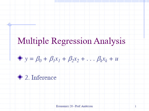
Multiple Regression Analysis
y = β0 + β1x1 + β2x2 + . . . βkxk + u 2. Inference
Economics 20 - Prof. Anderson
1
Assumptions of the Classical Linear Model (CLM)
2
Economics 20 - Prof. Anderson 6
The t Test (cont)
Knowing the sampling distribution for the standardized estimator allows us to carry out hypothesis tests Start with a null hypothesis For example, H0: βj=0 If accept null, then accept that xj has no effect on y, controlling for other x's
Economics 20 - Prof. Anderson 2
CLM Assumptions (cont)
Under CLM, OLS is not only BLUE, but is the minimum variance unbiased estimator We can summarize the population assumptions of CLM as follows y|x ~ Normal(β0 + β1x1 +…+ βkxk, σ2) While for now we just assume normality, clear that sometimes not the case Large samples will let us drop normality
《计量经济学导论》cha(1)

Pooling Cross Sections across Time: Simple Panel Data Methods
Chapter 13
Wooldridge: Introductory Econometrics: A Modern Approach, 5e
© 2013 Cengage Learning. All Rights Reserved. May not be scanned, copied or duplicated, or posted to a publicly accessible website, in whole or in part.
© 2013 Cengage Learning. All Rights Reserved. May not be scanned, copied or duplicated, or posted to a publicly accessible website, in whole or in part.
《计量经济学导论》ch

© 2012 Cengage Learning. All Rights Reserved. May not be scanned, copied or duplicated, or posted to a publicly accessible website, in whole or in part.
More on Specification and Data Issues
Chapter 9
Wooldridge: Introductory Econometrics: A Modern Approach, 5e
© 2012 Cengage Learning. All Rights Reserved. May not be scanned, copied or duplicated, or posted to a publicly accessible website, in whole or in part.
Multiple Regression Analysis: Specification and Data Issues
As expected, the measured return to education decreases if IQ is included as a proxy for unobserved ability.
Regression specification error test (RESET) The idea of RESET is to include squares and possibly higher order fitted values in the regression (similarly to the reduced White test)
- 1、下载文档前请自行甄别文档内容的完整性,平台不提供额外的编辑、内容补充、找答案等附加服务。
- 2、"仅部分预览"的文档,不可在线预览部分如存在完整性等问题,可反馈申请退款(可完整预览的文档不适用该条件!)。
- 3、如文档侵犯您的权益,请联系客服反馈,我们会尽快为您处理(人工客服工作时间:9:00-18:30)。
Multiple Regression Analysis: Specification and Data Issues
Testing against nonnested alternatives Model 1:
Which specification is more appropriate?
Model 2:
One may also include higher order terms, which implies complicated interactions and higher order terms of all explanatory variables
RESET provides little guidance as to where misspecification comes from
Multiple Regression Analysis: Specification and Data Issues
Tests for functional form misspecification One can always test whether explanatory should appear as squares or higher order terms by testing whether such terms can be excluded Otherwise, one can use general specification tests such as RESET
© 2012 Cengage Learning. All Rights Reserved. May not be scanned, copied or duplicated, or posted to a publicly accessible website, in whole or in part.
Define a general model that contains both models as subcases and test:
Discussion Can always be done; however, a clear winner need not emerge Cannot be used if the models differ in their definition of the dep. var.
© 2012 Cengage Learning. All Rights Reserved. May not be scanned, copied or duplicated, or posted to a publicly accessible website, in whole or in part.
More on Specification and Data Issues
Chapter 9
Wooldridge: Introductory Econometrics: A Modern Approach, 5e
© 2012 Cengage Learning. All Rights Reserved. May not be scanned, copied or duplicated, or posted to a publicly accessible website, in whole or in part.
Test for the exclusion of these terms. If they cannot be exluded, this is evidence for omitted higher order terms and interactions, i.e. for misspecification of functional form.
Multiple Regression Analysis: Specification and Data Issues
Using proxy variables for unobserved explanatory variables
Example: Omitted ability in a wage equation
Regression specification error test (RESET) The idea of RESET is to include squares and possibly higher order fitted values in the regression (similarly to the reduced White test)
© 2012 Cengage Learning. All Rights Reserved. May not be scanned, copied or duplicated, or posted to a publicly accessible website, in whole or in part.
Replace bபைடு நூலகம் proxy
In general, the estimates for the returns to education and experience will be biased because one has omit the unobservable ability variable. Idea: find a proxy variable for ability which is able to control for ability differences between individuals so that the coefficients of the other variables will not be biased. A possible proxy for ability is the IQ score or similar test scores.
Multiple Regression Analysis: Specification and Data Issues
Example: Housing price equation
Evidence for misspecification
Discussion
Less evidence for misspecification