THE PARTIAL EQUILIBRIUM COMPETITIVE MODEL(局部均衡竞争模型)尼科尔森中级微观ppt
经济——英文2

Contract Theory (WS 2003/04)
1-7
Prof. Dr. Klaus M. Schmidt
• Hidden information: The agent privately observes the realization of the state of the world (after the contract has been signed). Principal observes the agent’s action, but he does not know whether the action is appropriate. 2. Adverse Selection: Asymmetric information before the parties negotiate the contract. 3. Non-Verifiability: The involved parties are symmetrically informed and observe the state of the world, but they cannot verify it to the courts. → Incomplete Contracts. Note: Some authors use a different classification. For example, Laffont and Martimort identify “moral hazard” with “hidden action” and “adverse selection” with “hidden information”. Therefore, it is always crucial to ask what the information structure under consideration is.
A Model of Growth Through Creative Destruction A Model of Growth Through Creative Destruction

A Model of Growth Through Creative DestructionAuthor(s): Philippe Aghion and Peter HowittSource: Econometrica, Vol. 60, No. 2 (Mar., 1992), pp. 323-351Published by: The Econometric SocietyStable URL: /stable/2951599Accessed: 24/09/2009 08:00Your use of the JSTOR archive indicates your acceptance of JSTOR's Terms and Conditions of Use, available at/page/info/about/policies/terms.jsp. JSTOR's Terms and Conditions of Use provides, in part, that unless you have obtained prior permission, you may not download an entire issue of a journal or multiple copies of articles, and you may use content in the JSTOR archive only for your personal, non-commercial use.Please contact the publisher regarding any further use of this work. Publisher contact information may be obtained at/action/showPublisher?publisherCode=econosoc.Each copy of any part of a JSTOR transmission must contain the same copyright notice that appears on the screen or printed page of such transmission.JSTOR is a not-for-profit organization founded in 1995 to build trusted digital archives for scholarship. We work with the scholarly community to preserve their work and the materials they rely upon, and to build a common research platform that promotes the discovery and use of these resources. For more information about JSTOR, please contact support@.The Econometric Society is collaborating with JSTOR to digitize, preserve and extend access to Econometrica.。
比较优势理论(中英版)

6. Other assumptions:
1) Goods are identical(产品同质). 2) Perfect knowledge(信息完全). 3) No transport costs(没有运输成本). 4) No tariffs or other trade barriers(没有贸易壁垒).
E
QR
Chapter 2
Opportunity Cost and PPF
1. Opportunity Cost(机会成本)
• The cost of an activity in terms of sacrificed next best alternative uses of the assets involved. Can also be formulated as “amount of product 2 we must give up to produce a unit of product 1” .
Home’s PPF: aLCQC+ aLwQw≤ L
Chapter 2
QW
· L/aLW
=
•当本国完全生产奶酪时,QC=L/aLC •当本国完全生产葡萄酒时,QW=L/aLW
•生产一单位奶酪的机会成本是: QW /QC= aLC /aLW
Chapter 2
1. One input(单一要素): Labor(L)
2. Two outputs: Wine (Qw) and Cheese(Qc) 3. Two countries: Home and Foreign(*)
《高级宏观经济学》教学大纲(硕士研究生)-RonaldoCarpio

《高级宏观经济学》教学大纲(硕士研究生) - RonaldoCarpio《高级微观经济分析》教学大纲(博士研究生)课程代码:(按本专业或方向培养方案填写)课程名称:(按本专业或方向培养方案填写)英文名称:Advanced Microeconomic Analysis课程性质:(按本专业或方向培养方案填写)学分学时:3学分,48学时授课对象:金融学院一年级博士研究生课程简介:Based on Microeconomics I (for master students), the course will discuss thecontemporary development in microeconomics. This course is also designed to develop andextend the students’ analytical and reading skills in modern microeconomics. A student who haspassed the course should be able to read typical articles in the mainline journals, understand theanalytical derivations and arguments commonly used in the literature, and know how to solve themore widely used models.先修课程:Microeconomics for master students选用教材:1、 Mas-Colell, A., M. D. Whinston, and J. Green, Microeconomic Theory. (MWG)2、 Jehle, Geoffrey A. and Philip J. Reny, Advanced Microeconomic Theory. (JR)考核方式与成绩评定:Final Exam %; Midterm Exam %; Class Participation % 主讲教师:Carpio Ronaldo、颜建晔所属院系:金融学院联系方式:******************、*******************答疑时间及地点:求索楼123,Wednesday 13:30-14:30 (Carpio),Tuesday 15:00-17:00(颜)第一章:Consumer Theory教学目标和要求:Understand the consumer’s problem and consumer demand.教学时数:6学时教学方式:讲授准备知识:calculus教学内容:Preferences, Utility, and Consumer’s Problem第一节:Consumer’s Problem第二节:Indirect Utility, Demand作业与思考题:JR Ch 1.6参考资料:JR Ch 1, Appendix A1, A21第二章: Topics in Consumer Theory教学目标和要求:Understand duality, integrability, and uncertainty.教学时数:6 学时教学方式:讲授准备知识:statistics教学内容:Duality, Integrability, and Uncertainty 第一节:Duality of Consumer’s Problem第二节:Revealed Preferences & Uncertainty 作业与思考题:JR Ch 2.5 参考资料:JR Ch 2第三章: Theory of the Firm教学目标和要求:Understand the firm’s profit maximization problem.教学时数:6 学时教学方式:讲授准备知识:Chapter 1,2教学内容:Production, Cost, Profit Maximization 第一节:Production Functions & Cost第二节:Duality in Production, Competitive Firms 作业与思考题:JR Ch 3.6参考资料:JR Ch 3第四章: Partial Equilibrium教学目标和要求:Understand partial equilibrium markets. 教学时数:3学时教学方式:讲授准备知识:Chapter 3教学内容:Perfect & Imperfect Competition, Welfare 第一节:Competition 第二节:Equilibrium & Welfare作业与思考题:JR Ch 4.4参考资料:JR Ch 4第五章: Walras’/competitive equilibrium2教学目标和要求:competitive market economies from a Walrasian (general) equilibrium perspective.Let students understand “why the competitive market/equilibrium may work or fail?”教学时数:6学时方式:讲授教学准备知识:consumer theory, production theory教学内容:第一节:Walrasian economy and mathematical language of microeconomics 第二节:competitive equilibria of pure exchange and with production 作业与思考题:JR5.5, exercises of MWG Ch15, 18, 教师自编习题集参考资料:MWG Mathematical Appendix, Ch15, 18; JR5.4第六章: Social choice function/theory and social welfare: normative aspect of microeconomics教学目标和要求:When we judge some situation, such as a market equilibrium, as “good”or “bad”, or “better” or “worse” than another, we necessarily make at least implicit appeal to some underlying ethical standard. Welfare economics helps to inform the debate on social issues by forcingus to confront the ethical premises underlying our arguments as well as helping us to seetheir logical implications.Let students have a systematic framework for thinking about normative and social welfare topics.教学时数:3学时教学方式:讲授准备知识:Walrasian equilibrium教学内容:第一节:social choice, comparability, and some possibilities第二节:Rawlsian, Utiliterian, and flexible forms作业与思考题:JR6.5, exercises of MWG Ch21, 22, 教师自编习题集参考资料:MWG Ch21.A, Ch21.E, Ch22.C; JR Ch6第七章: Strategic Behavior and Asymmetric Information教学目标和要求:A central feature of contemporary microeconomicsafter Walrasian economy is the multi-agent interaction which represents the potential for the presence of strategicinterdependence. Let students grasp classic models of imperfect competition under symmetric and asymmetric information.3教学时数:3学时教学方式:讲授准备知识:perfect competition教学内容:第一节:monopoly and oligopoly under symmetric information第二节:oligopoly under asymmetric information作业与思考题:教师自编习题集参考资料:MWG Ch12; JR Ch4第八章: Theory of Incentives教学目标和要求:The strategic opportunities that arise in the presence of asymmetricinformation typically lead to inefficient market outcomes, a form of market failure. Underasymmetric information, the first welfare theorem no longer holds generally. Thus, the main themeto be explored is to stimulate different agents’ optimal/efficient behaviors in differentinformational settings to achieve the “second-best” market outcomes.教学时数:9学时教学方式:讲授准备知识:Strategic Behavior and Asymmetric Information教学内容:第一节:Adverse selection第二节:Moral hazard*第三节:Task separation/integration,第三节:Career concern作业与思考题:exercises of MWG Ch13, 14, 教师自编习题集参考资料:JR Ch8; MWG Ch13, 14第九章前沿研究讲座:待定邀请校外老师(待定)给学生们讲演最新研究,引导学生讨论;在学生掌握现代微观经济学基本模型之后能够接触到前沿研究。
大学生论文旅游发展外文文献
Measuring the Impact of Tourism upon Urban Economies:A Review of LiteratureKTHC – Knowledge, Technology, Human CapitalUgo Gasparino, Elena Bellini, Barbara Del Corpo and William MaliziaAbstractTourism is increasingly seen as a potential lever towards high economic growth, measured both in terms of income and employment. In recent years, interest in tourism has spread rapidly throughout many small and medium European cities, which previously have not considered themselves as tourist destinations. This paper reviews and summarizes the existing literature on the economic assessment of tourism with the objectives of, firstly, identifying the main categories of impacts and, secondly, constructing an inventory of methodologies available to assess them. We will progress step by step, starting from the most simplistic approaches and relaxing assumptions as we proceed. Firstly, we assume a static setting, with spare capacity. In such a setting (partial equilibrium), prices do not respond to demand shocks: only quantities (production, income and jobs) adjust. Secondly, we relax this assumption and assume that there is no spare capacity: prices respond to increasing demand (general equilibrium), leading to reallocation of resources across sectors. We then move from a static to a dynamic setting and survey those contributions that look at the relationship between tourism specialisation and long-run growth.Keywords: Tourism, Economic Impacts, Input-Output Analysis, General and PartialEquilibrium Analysis1 The partial equilibrium analysisPartial equilibrium analysis assumes that there is spare capacity unemployed resources and that, as a consequence, prices do not respond to increasing demand (perfect elastic supply). Adjustment takes place only through quantities (production, jobs, and therefore income).The basic concept of partial equilibrium analysis is that of ‘multiplier’ although, as noticed by Archer, «there is perhaps more misunderstanding about multiplier analysis than almost any other aspect of tourism research» (Archer, 1982). Multipliers measure the present economic performance of the tourism industry and the effects of short-run economic adjustments to a change in the level of tourist expenditure.The definition of multiplier, in terms of Keynes, is unequivocal: the multiplier measures the increase in economic activity generated in an economy by a unit increase in tourism expenditure. A tourism income multiplier is a coefficient that expresses the amount of income generated in an area by an additional unit of tourist spending: for instance, if tourists spend an extra EUR 1 million in the area and this generates EUR 800,000 of income, the Keynesian multiplier is 0.81. However, alternative definitions of multipliers can be found in tourism literature. The most popular of these is the use of ‘ratio’ multiplier, where for example the income multiplier tends to be expressed as the ratio of a ‘total’ income generated by tourism expenditure (see Section 1.1) to the ‘direct’ income. Depending on what is meant by ‘total’ income, three types of ‘ratio’ multipliers can be generated.Despite the strong assumptions implicit in their calculation, multipliers are widely used in policy-making. They are used to study the impact of tourism on business turnover, income and employment and can be used to compare the impact of increased demand on other sectors of the economy or different policy options.In what follows, we firstly introduce the economic meaning of multipliers, analysing how the tourist expenditure ripples through the economy. Secondly, we present two widely used methodologies to calculate multipliers. Finally, we briefly discuss and compare some of the empirical results.2 The economic meaning of multipliersIn the destination tourists spend their money to buy certain goods and services. This initial tourist expenditure is generally directed to very specific sectors of the economy (lodging, restaurant, amusement, retail trade, transportation – which we will refer to asAlthough the correct methodology would require the calculation of the multiplier at the margin, it is common practice (mainly because of data limitation) to calculate income effects in terms of average, rather than marginal, tourism expenditure and to assume that there is no significant difference between them. This implies that the economy has available capacity to meet future demandTourism industries and represents additional revenues for these activities. These are the so-called direct effects.Part of those revenues is used to buy intermediate goods and services that will be used in ‘future production cycles’ (intermediate demand). A remaining part will be used to buy the services of production factors: labour, capital and land (wages, interests and profits, and rents –gross value added), to pay taxes to central and local governments, or saved. In all cases,some money could go outside the area, to intermediate producers and production factors located outside the area (i.e., it ‘leaks’ out of the local economy).However, some will remain within the area: local tourism industries will hire new local workers (paying a bigger number of wages) and demand additional goods from local producers. As a result, local output increases, employment opportunities increase and local income rises (due to the increase in the number of wages). These are the so-called indirect effects.The increase in employment brings to an increase in the total income of local residents.Part of this income is saved and part is spent in consumption goods. This in turn generates additional demand which, as before, translates into additional production and employment (and so on). These are the so-called induced effects. Indirect and induced effects are often called secondary effects. The effect of tourism on the local economy is influenced by a few key factors: The characteristics and the spending patterns of the local tourists, affecting the direct impact on the economy. Essential features here include: The reason for travel (tourists travelling for cultural reasons spend more/less and put more/less pressure on natural and cultural resources than sun&beach tourists);The length of stay (tourists staying for the day are likely to spend a smaller share of total expenditure in locally produced goods); The accommodation chosen (hotels are more expensive than campsites).The characteristics of the tourism industries and of the local economy. Key features here include the ability of local economy to satisfy the demand of tourism industries, as well as the size and the shares of tourism industries that are locally owned. The extent of the indirect effects depends on the size of the area under study (e.g., municipal, regional, national) and on the extent to which business firms in the area supply each other with goods and services (the more likely the more diversified and interlinked is the local economy). In general, the smaller the scale of the economy and the higher the share of initial expenditure that leaks out of the local area, the fewer are these linkages and the smaller are the indirect effects. Moreover, the magnitude of indirect and induced effects depends on the share of capital, land and labour that is locally owned. For instance, small family-owned hotels and restaurants are more likely to buy local intermediate inputs than chain hotels and tourist villages. If factors are locally owned, their remunerations – profits, rent and wages – will stay locally and local community will strongly benefit from them.3. Direct, indirect and induced benefits and effects on the economytriggered by touristSpending Several types of multiplier are commonly used:Sales (or transactions) multiplier refers to the effect on business turnover (value of business turnover created by a unitary increase in tourism expenditure); Output multiplier refers to the effect on the level of output of the economy. With respect to the sales multiplier it does not only take into account the impact on turnover of local businesses, but also any changes in the level of stocks they hold. This can be useful in identifying potential supply shortfalls, or bottlenecks; Government revenue multiplier refers to the effects on governmental revenues from all sources (e.g., direct and indirect taxation, duties, licenses and fees); Income multiplier refers to the effect on incomes (sales net of intermediate consumption, including wages, salaries and profit). This is commonly regarded as the most important indicator of the economic performance of tourism industry. Income multipliers vary depending on whether they include or not incomes accruing to nonnationals residing in the region under investigation, and whether they include or not income accruing to governments. The multiplier can be measured as disposable income –the income available to individuals to spend or save, which is net of tax – or value added income – the income which includes tax and other expenditures which are defined according to national income accounting rules; Employment multiplier refers to the effect on employment. It is usually derived from the output or income multipliers. It can be expressed as the ratio of the number of ‘total’ additional jobs (e.g., direct and indirect or direct and secondary) to either the number of direct jobs (‘ratio’ multiplier) or to the initial tourist expenditure(Keynesian multiplier). Employment can be measured in terms of full time equivalent jobs, or the actual number of jobs including part-time jobs.Suppose additional tourist expenditure of EUR 1 million generating EUR 2.5 million of extra output and EUR 500 000 of direct and secondary income. It also creates 200 jobs directly and 180 secondarily. In Keynesian terms the multipliers are, respectively: 2.5 (output), 0.5 (income) and 3.8 jobs for 10 000 EUR of tourist expenditure (employment).On the other side employment, in terms of ‘ratio’ multipliers (i.e., total employment generated to direct employment) can alternatively be expressed as 1.9 (i.e., 380/200).The various multipliers are inextricably linked to each other. Sales and Output multipliers have limited use from the policy point of view, except as an indicator of the degree of economic internal linkages. On the other side, it is important for policymakers to be aware of the income and employment effects of any anticipated changes in final demand, makingincome and employment multipliers the most often quoted types of multipliers.Multipliers are not only influenced by the economy and tourism characteristics of the area of concern, but they also reflect its size (and population). Studying the impact of local tourism one of the most common errors, when the available resources do not allow independent and consistent estimations, is to ‘borrow’ multipliers evaluated at national scale (or in areas erroneously considered to be ‘equivalent’ to the area of concern) and to apply them uncritically to sub-national areas (e.g., municipalities, regions). The use of national multipliers tends usually to yield inflated estimates of impacts.The model is static and assumes that there are (unlimited) idle resources (including labour, natural resources and capital goods), which means that any increase in final demand can simply be met by proportionally increase in sectoral outputs. As a consequence, prices do not respond to increasing demand (perfect elastic supply) and the growth of tourism do not lead to a reallocation of resources across sectors. Even granted that in most economies there is some unemployment of labour, this assumption seems rather unlikely. The ability of the economy of a study area to respond immediately to changes in final demand (i.e., the absence of capacity and supply constraints) has seriously been questioned by many researchers (Briassoulis, 1991);Technologies are fixed. All firms in each sector employ the same technology, and there are neither economies nor diseconomies of scale and no substitution among inputs;The outputs of each sector are homogeneous. An industrial sector cannot increase the output of one specific product unless it proportionally increases the output of all its other products;In calculating the employment effect, the model assumes a fixed employment/output ratio. Productivity increases are not taken into consideration (any additional demand for labour translates into a proportional increase in the number of employees);It is a ‘data hungry’ methodology, a s it relies on the existence and availability of a reliable case study-specific I-O matrix;The I-O matrix approximates the actual economy with respect to the year it is estimated. The farther away we are from the I-O table year, the less the evaluation corresponds to actual economy. Tourism, as any economic activity, passes through several stages during its development. The early stages of tourist development of an area are characterized by dynamic, short-term changes implying that technical coefficients do not remain stable at least for some period. Furthermore, tourism can induce developments and infrastructures in the host region that otherwise would not probably occur. As a tourist region matures, the assumption ofconstant coefficients may be more acceptable (but the coefficients cannot be assumed to remain constant for time periods longer than, typically, five years). At the level of multipliers, it has to be noticed that the income multiplier, expressed as ratios of money to money may not significantly change over time; Keynesian employment multiplier, however, being expressed as a ratio of number of employees to tourism expenditures, will be affected by inflation. These limitations become increasingly binding the greater the simulated change in demand. Although real world production relationships are most probably non-linear, it is not unreasonable to approximate these with linear specifications as long as the changes from the starting point remain relatively small. On the other hand, simulations that involve drastic changes from the means are likely to have poor predictive abilities.Despite of these limitations, an understanding of the caveats can help the analyst to overcome the weaknesses.Depending on the characteristics of the area of concern and on the tourist spending patterns, the assumptions at the base of I-O analysis could bias the values of the derived tourism multipliers (Fletcher, 1989; Briassoulis, 1991). As already noticed, for the employment multiplier values to hold true, it must be assumed that an increase in final demand will result in each sector increasing their demand for labour in a linear way. This will only be reasonable if every sector is operating at full utilization. Any underutilization will mean that sectors can expand output without resorting to employing additional staff. In the short run it is likely that most sectors will meet additional demand by either better utilization of existing personnel or by increasing over-time. In such cases, the employment multiplier will over-estimate the effects on employment. This can be particularly critical in the case of tourism, where the restaurant & hotel industry is typically characterized by capacity under-utilization (reflected in hotel occupancy rates lower than 100%). This means that additional tourists can be accommodated by existing hotels and restaurants with only a marginal increase in employment and in the inputs required from the other sectors of local economy. Further difficulties inherent to the assessment of employment impacts are related to seasonality problems (particularly important for sun&beach tourism) and to the fact that it is very common in tourismrelated establishments that many people employed in tourism also hold another job and part-time employment.Furthermore, it is also quite conceivable that some industries will not be able to respond to an increase in demand (particularly in the short-term run) and any increase in demand will need to be met by an increase in imports rather than an increase in the level of output of thedomestic industries.There is a wide range of literature on (tourism) multipliers. We do not aim at discussing all findings, but rather at identifying those factors that influence the values of multipliers and that might be relevant to our discussion. We will firstly discuss issues relative to the calculation of multipliers. This part will help to clarify some of the definitions presented in previous sections and to assess the range of changes involved with the different definitions. Secondly, we will discuss issues relative to the destination regions (and how they influence the value of multipliers). This will help to clarify the regional factors that we need to take into consideration in the empirical studies. Thirdly, we will discuss the relevant features of tourism and tourists’ patterns. This is very relevant for policy-making in the field of tourism; different strategic choices must be compared. Finally, we willdiscuss the issues concerning the impact on employment.Caution must however be exercised when comparing quantitatively multipliers from different studies, since multipliers might have been generated by different methodologies, include different assumptions, reflect different distributions of expenditures (e.g., more on hotel, less on shopping).Types of multiplier and their range of values.Multipliers have been widely used in research and policy support. However, their use has been often characterized by confusion and misunderstanding concerning the typologies of the used multipliers (Archer, 1982). Here we discuss the range of changes in empirical findings involved when different typologies of multipliers are used.A first distinction refers to the range of effects taken into account by the multiplier. In Singapore, income and output multiplier increase by 30% when induced effects are included (Heng and Low, 1990); the increase in the income multiplier, when also induced effects are considered, is found by Del Corpo et al (2008) to vary from 20% in Sicily to 65% in Spain. Feedback effects from surrounding regions can also be considered. Sinclair and Sutcliffe (1988) take into account feedback effects from surrounding economies and show that the size of multiplier increases by 2-7%.The second distinction refers to the affected variable (sales, output, income or employment multiplier). This is a simple and clear issue, but it is very relevant when comparing different values of multipliers. It is important to note that different definitions of multipliers are relevant for different policy objectives. The relevant multipliers should be therefore chosen when comparing different policy options with respect to a specific objective (either themaximisation of the employment, income or government revenues effect). Sales and output multipliers tend to be around the double of income multipliers (Heng and Low, 1990). Multipliers and features of destination regionThe value of the multipliers crucially depends on leakages, and therefore on the share of imports to total output. In turn, the share of import is heavily dependent on the size of theregion (small economies are relatively less self-contained than larger economies). In the specific case of tourism multipliers, the interrelationships of tourism industries with the rest of the local economy (and specifically the extent to which demand from tourism industries is satisfied with imports), is also a crucial factor.Income multipliers reach a maximum for large countries such as Turkey and the UK and in self-contained small island economies (Jamaica, Mauritius), where they vary in the range 0.50-1.20. They are just smaller for US states (range 0.40-0.90 – Archer, 1988), but sensibly lower in very open regional and urban economies such as US and UK counties (range 0.20-0.50 –Fletcher, 1989; Archer, 1982). Baaijens et al (1998) analyzed statistically (regression models) income multipliers extracted from 11 studies. A positive relationship was found with the logarithm of the population (several alternative regional characteristics –as area size, number of tourist arrivals – were also tested). A similar result was found by Chang (2001), analyzing more than 100 regional IO models varying in size and economic development (covering five US-states: California, Colorado, Florida, Michigan and Massachusetts), generated by means of the IMPLAN I-O modelling system. A ‘tourism multiplier’ was defined as a weighted sum of multipliers derived from four tourism-related sectors (lodging, eating and drinking, recreation and retail). For all the four analyzed Type II ‘tourism multipliers’ (sales, income, value added and job) the most significant predictor, in a stepwise regression analysis, was found to be the logarithm of population. While sales, income and value added multipliers increased almost linearly with the logarithm of population, the employment multiplier showed a negative correlation (interpreted on the basis that, in the contest of the analyzed dataset, regions characterized by a smaller number of inhabitants tend to correspond to less economically developed rural areas). Using hotels as an example, higher job to sales ratio could be a result of lower room rates, or more part-time and seasonal jobs (resulting in lower average wages).Type II multipliers vs. Log (Population) for 114 US regions. The empty diamonds report the results obtained through I-O modelling (IMPLAN), while the squares correspond to the corresponding results from a statistical regression analysis with Log (Population) as dominantpredictors. The lines report empirical multipliers proposed from a straightforward classification of the different regions in: ‘rural’, ‘small me tro’, ‘large metro’ and ‘State’. Multipliers and features of tourism and tourists’ patternsTourists differ in behavioural and expenditure patterns. This has consequences for the size and range of economic effects. This question is crucial when confronting different policy choices for tourism development (e.g., privileging short vs. long stays, beach resort vs. cultural tourism, etc.). Two key issues must be taken into account here.Firstly, the impact on the local economy varies not only depending on the value of the multipliers, but also on the value of the multiplicand: even if the multiplier is high, the final impact on local income will be low if the direct injection of tourist expenditure in the destination region is low. Previous research shows that tourist spending taking place through tour operators, international airlines and chain hotels often leaks out immediately without even reaching the destination economy. For example, only 42% of the price of a package holiday was received by Spain when tourists travelled on a non-Spanish airline (Istituto Espanol de Turismo, 1987). Similar results hold for Kenya: only 38% of UK tourists’ spending travelling in package holidays reached Kenya.Improving options locally available to tourists would magnify the size of economic impacts. In the case of Kenya, the use of local airlines could considerably increase the share of expenditure accruing to the Country: up to 66% if local airlines are used for internal travels, up to 80% if Kenyan airlines are used for international flights also (Sinclair, 1991). Secondly, the impact on the local economy varies with the patterns of tourist’s expenditure, in turn influenced by the motivation of the trip (pleasure vs. business, for example), the nationality of tourists, the accommodation chosen. Research shows that accommodation is a key factor, as confirmed among others by Del Corpo et al (2008). Sinclair and Sutcliffe (1988) find that the income multiplier in Malaga is lower for tourists staying in flats or villas and higher for tourists staying in hotels. This is due to the different relationships that these types of accommodation create with the local economy.On the contrary, the nationality of the tourist does not seem to be so relevant. Archer and Fletcher (1996) find no evidence that nationality of tourists made a significant difference to the size impact of tourism on the economy of Seychelles. The difference is found to be negligible also in the three case studies used by Del Corpo et al (2008), that is Bergen, Elche and Syracuse, even though in general Spanish tourists in Elche present a higher direct impact than foreigners. Finally, Heng and Low (1990) find no evidence that tourists from developingcountries had a different impact than tourists from developed countries.The impacts on employmentThe ability of tourism to create jobs is of high relevance for policy-makers.As discussed in Section 1.1, employment multipliers are easily calculated in multiplier exercises. The values of the multiplier are influenced by the same factors discussed in previous sections, and therefore differ quite widely. Heng and Low (1990) find that tourism in Singapore creates over 30 jobs per million dollar of expenditure when induced effects are included and just above 25 jobs when only direct and indirect effects are calculated. Fletcher (1989) finds a similar value for Jamaica. He shows that values might be even higher for smaller economies such as Gibraltar, where he also finds that the employment multiplier of tourism expenditure is nearly the double than Ministry of Defence and other Government departments’ expenditure.Sinclair (1998) discusses few additional features concerning employment effects of tourism (based both on case studies and multiplier analysis):Tourism industries are relatively skill-intensive. This was pointed out by Diamond (1974), in his research on Turkey, and confirmed by following studies. Delos Santos etal (1983) further noticed that only 16% of employment in the tourism sector in the Philippines was unskilled and that nearly 40% was semi-skilled;Much of the employment in the catering and accommodation is on a part-time seasonal basis or family-related without a formal wage. Sinclair and Bote Gomez (1996) find that just below 10% of part-time workers in hotels and guesthouses in Spain were without a formal wage. Farver (1984) finds that hotel employment in Gambia nearly doubled in the high season with respect to the low season. He also finds that top managerial posts are usually occupied by foreigners. This appears to be true also for the Fiji Islands (Samy, 1975). However, in Kenya this trend has been reversed and top managerial posts are now being taken by residents (Sinclair, 1990).These results point out to potential important employment gains from tourism, under both a quantity and a quality perspective (although seasonality remains a problem).4 ConclusionsBased on the review of literature, we can propose a rather general classification of the impacts of tourism on urban economies:The impacts that take place through market interactions;The impacts that do not involve market interactions;The key issues that affect the size and sign of the impacts.4.1 Impacts taking place through market interactionsTourists typically demand a set of services and goods. Some of these are provided by the market, such as restaurants, hotels, private transportation (we referred to them as tourism industries). This additional demand generates a series of impacts on the local economy: Increased expenditure by tourists increases local production (and incomes). Assuming that there is idle capacity (and prices do not respond to increased demand), the final increase is bigger than the initial increase (multiplier effect);The additional income brings with it additional jobs: directly, in the tourism sector and indirectly in the sectors serving the tourism sector;When relaxing the assumption of idle capacity, prices (as well as quantities) respond to the additional demand. Theory shows that, finally, the benefits of tourism are capitalized in higher prices of non-tradable sectors (hotels, restaurants, houses, prices of locally produced goods) and that they finally accrue to the immobile factors (e.g., land) employed in the non-tradable sector (which is able to charge higher prices).The above effects imply that there is a distributional issue, as tourism leads to a contraction of the traded sector (e.g., manufacturing) and to a decrease of real returns to all the other factors; The structural change induced in the economy may affect its capability to grow in the long run. The crucial question is whether a region relatively specialized in tourism will grow slower or faster than, for example, regions specialized in knowledge intensive industries. Theoretically, the answer depends on the long-run dynamics of prices of tourist goods compared to, for example, knowledge-intensive goods.4.2 Impacts taking place through non-market interactionsTourists do not only demand goods and services provided by the market. They also demand access to natural and cultural resources and to publicly provided goods and services (such as water, public transportation, health and security, a clean environment).This additional demand generates the following impacts.Firstly, the additional pressure on natural and cultural resources can lead to their overexploitation and degradation.Secondly, the pressure on public services will also increase, as a consequence of the additional demand for water, waste and water treatment, public transportation. The additional costs will be compensated (to some extent) by an increase of fiscal revenues following the increase of incomes and jobs.。
第二章:比较优势理论

2006年版
CHAPTER 2
Chapter 2
Comparative Advantage Model
2006年版
Chapter 2
Limitation of the Smith’s Model
10*30=300 0*25=0
0*30=0 10*25=250
510 520 500
Chapter 2
Best Cooperation in Family
1. So, the best division of labor in one family is that women doing housework and men going out for work.
2. Partial Equilibrium Analysis局部均衡法
1) PEA means only analyzing single market in one time 2) We usually use the Demand Curve and the Supply Curve
as the basic tools in the partial equilibrium analysis.
Labor
Goods Cloth
Wheat
Productivity
Cloth Wheat
Home 100 100 50 1 0.5
Foreign 100 18500 100 1.5 1
In this case, Foreign has the absolute advantage in both goods (it is very common for a developed country to have absolute advantages in most sectors). According to the Smith theory, there will be no trade.(Really?)
经济学专用名词解释
~Equilibrium,competitive 竞争均衡见竟争均衡(competitive equilibrium)。
Equilibrium,general 一般均衡见一般均衡分析(general-equilibrium analysis)Equilibrium,macroeconomic 宏观经济均衡意愿总需求等于意愿总供给的GDP水平。
在均衡时,意愿的消费(C),政府支出(G),投资(I)和净出口(X)的总量正好等于在当前价格水平下企业所愿意出售的总量。
Equimarginal principle 等边际法则决定收入在不同消费品之间分配的法则。
消费者可按此法则选择消费组合,使花费在所有商品和服务上的每一美元的边际效用都相等,就能保证消费者所获得的效用最大化。
Exchange rate 汇率见外汇汇率(foreign exchange rate)Exchange-rate system 汇率制度国家之间进行支付时所依据的一组规则、安排和制度。
历史上最重要的汇率制度是金本位制、布雷顿森林体系和现在的浮动汇率制。
Excise tax vs.sales tax 消费税和销售税消费税是对某种或某组商品,如酒和烟草的购买所课征的税。
销售税是对除少数特定商品(如食品)以外的所有商品所课征的税。
Exclusion principle 排他原则私人品区别于公共品的一种性质。
当生产者将一种商品卖给A 后,若能很容易地将B、C、D等人排除在该商品益处享用过程之外,则排他原则就在发生作用,该商品也因此是一项私人品。
若不能轻易地把其他人排除在分享过程之外,如公共卫生或国防,则我们称该商品具有公共品的特征。
Exogenous vs.induced variables 外生变量和引致变量外生变量是那些由经济体系以外的因素来决定的变量。
与外生变量相对应的是引致变量,后者是由经济体系的内在运行所决定的。
例如,天气变化是外生变量,而消费的变化则常常由收入变动所引致。
微观经济学理论部分英文词汇
46, sequences
n. [数][计] 序列,顺序;继起的事(sequence的复数形式)
Sequences: 序列 | 图形逻辑 | 数列
47, semester [sɪ'mestə]
n. 学期;半年
48, relatively ['relətɪvlɪ]
Reunited: 重遇 | 重聚 | 团聚
9, proofs [pru:fs]
n. 证明;证据(proof的复数);校稿
10, proceeds ['prəʊsiːdz]
n. 收入,收益;实收款项
11, extension [ɪk'stenʃ(ə)n; ek-]
n. 延长;延期;扩大;伸展;电话分机
n. 筛选;放映;[物] 屏蔽;审查;防波
v. 筛选;拍摄(screen的ing形式);遮蔽;隔挡
Screening: 场次 | 筛选 | 筛查
56, mechanism design
机制设计(微观经济学和博弈论的分支领域);机构设计(学科名称);机械设计
57, altered ['ɔːltəd]
27, Fixed Point Theorems
Fixed Point Theorems: 不动点定理
28, coverage ['kʌv(ə)rɪdʒ]
n. 覆盖,覆盖范围
coverage: 新闻报道 | 覆盖面 | 保险范围
29, instructors
n. 教练;讲师;指导书(instructor的复数)
adj. 人际的;人与人之间的
绝对优势理论
绝对优势理论张五常前面极尽详细地介绍了“重商主义”的产生背景、观点主张与政策建议、错误所在。
在分析“重商主义”的错误时,我们只是从货币理论的角度指出重商主义者把黄金等同于财富是错的,以及贸易顺差的不可持续性,却未对他们的另一个重要观点“贸易是损人利己的零和游戏”作出批判。
这是因为有关的批判要留到这里介绍亚当·斯密的“绝对优势理论”再进行。
事实上,斯密的这个理论,就是为了针对重商主义的这个错误而提出的。
我们先看一个局部均衡(Partial Equilibrium)的分析,再转向能直接反映斯密的“绝对优势理论”的一般均衡(General Equilibrium)的分析。
所谓局部均衡分析是指只分析市场的一个局部,其它部分归为“其它因素不变”之列。
而一般均衡分析则是指将所有因素都考虑在内,没有假设为不变的其它因素。
严格来说,这世上不可能、也没必要进行真正的一般均衡分析,因为世界上的局限条件如此之多,全部考虑在内既不可能、也没必要。
所以,所谓的局部均衡和一般均衡都只是相对而言。
具体到国际贸易的领域,所谓的局部均衡分析是指只分析一种产品的情况,而一般均衡分析是指分析两种产品的情况。
那么,我们先来看局部均衡分析。
下图画的就是局部均衡分析的情况。
这分析把整个世界分为两部分:其一是美国,其二是美国之外的其它国家。
古典与新古典的国际贸易理论都使用两个国家的模型,这假设乍一看很远离事实,但并非如此。
一方面,两个国家的假设可以在解出基本模型之后放宽到多个国家;另一方面,只要把本国之外的所有其它国家看成是一个国家,则两国模型无需放宽有关假设都能反映现实。
这里有三个图,最左边的是美国的国内市场——由于这书是美国人写的,所以拿美国为例,一般化地说,左图反映的是进口国的国内市场;最右边的是其它国家的国内市场,一般化地说,那反映的是出口国的国内市场;中间的图是世界市场。
中间的图是从左图和右图推导出来的,因此我们要先看懂左图和右图,才能明白中间的图。
国际经济学名词解释
自给自足的相对均衡价格(equilibrium-relativecommoditypriceinisolation):在生产和消费那一点上一国生产可能性曲线和社会无差异曲线公切线的斜率。
贸易条件下的相对均衡价格(equilibrium-relativecommoditypricewithtrade):两国贸易平衡时贸易双方共同的均衡价格。
不完全分工(incompletespecialization):一国并不是花费所有的资源和技术生产其具有比较优势的产品,而是同时生产一部分不具有比较优势的产品。
提供曲线(offercurve):反映了一国为了进口的某一需要的商品数量而愿意出口的商品数量。
它具备了需要和供给两方面的因素。
贸易条件(termsoftrade):一国出口商品的价格和进口商品价格的比值。
在两国条件下,一国的贸易条件是另一国贸易条件的倒数。
在不止两种商品的贸易世界中,贸易条件是指一国出口商品价格指数和进口商品价格指数的比值。
要素密集度(factorintensities):是指生产一个单位某种产品所使用的生产要素的组合比例。
在资本与劳动两种生产要素的情形下,要素的密集度就是指生产一单位该产品所使用的资本-劳动比率。
要素丰裕度(factorabundance):要素丰裕度是一国的资源拥有状况,即一国的要素禀赋状况。
派生需求(deriveddemand):对一种生产要素的需求来自(派生自)对另一种产品的需求,其中该生产要素对这一最终产品会作贡献。
赫克歇尔-俄林定理(Hechscher-Ohlintheorem):一国应该出口该国相对便宜和丰裕的要素密集型的产品,进口该国相对昂贵和稀缺的要素密集型的产品。
要素比例或要素禀赋理论(factor-proportionsorfactor-endowmenttheory):一国应该出口该国相对便宜和丰裕的要素密集型的产品,进口该国相对昂贵和稀缺的要素密集型的产品。
- 1、下载文档前请自行甄别文档内容的完整性,平台不提供额外的编辑、内容补充、找答案等附加服务。
- 2、"仅部分预览"的文档,不可在线预览部分如存在完整性等问题,可反馈申请退款(可完整预览的文档不适用该条件!)。
- 3、如文档侵犯您的权益,请联系客服反馈,我们会尽快为您处理(人工客服工作时间:9:00-18:30)。
– An individual’s demand for x is
Quantity of x demanded = x(px,py,I) – If we use i to reflect each individual in the market, then the market demand curve is
18
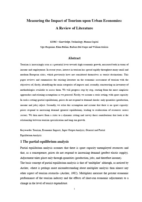
Short-Run Market Supply Curve
To derive the market supply curve, we sum the quantities supplied at every price
P Firm A’s supply curve
sA
P
sB
Firm B’s supply curve
3
Market Demand
To derive the market demand curve, we sum the quantities demanded at every price
px Individual 1’s demand curve px Individual 2’s demand curve px Market demand curve
8
Generalizations
• Suppose that there are n goods (xi, i = 1,n) with prices pi, i = 1,n. • Assume that there are m individuals in the economy
• The j th’s demand for the i th good will depend on all prices and on Ij xij = xij(p1,…,pn, Ij)
7
Shifts in Market Demand
• If py rises to 6, the market demand curve shifts outward to X = 27 – 3px + 4 + 1 + 6 = 38 – 3px
– note that X and Y are substitutes
Qs (P,v ,w ) qi (P,v ,w )
i 1 n
• Firms are assumed to face the same market price and the same prices for inputs
20
Short-Run Supply Elasticity
Price
S
When quantity is fixed in the very short run, price will rise from P1 to P2 when the demand rises from D to D’
P2
P1 D’ D
Q*
Quantity
15
Short-Run Price Determination
and individual 2’s demand is x2 = 17 – px + 0.05I2 + 0.5py • The market demand curve is X = x1 + x2 = 27 – 3px + 0.1I1 + 0.05I2 + py
6
Shifts in Market Demand
px* x1
x2
X
x1*
x
x2*
x
X*
x
x1* + x2* = X*
4
Shifts in the Market Demand Curve
• The market demand summarizes the ceteris paribus relationship between X and px
– changes in px result in movements along the curve (change in quantity demanded)
– the amount supplied by each firm depends on price
• The short-run market supply curve will be upward-sloping because each firm’s short-run supply curve has a positive slope
11
Elasticity of Market Demand
• The cross-price elasticity of market demand is measured by
eQ,P QD (P, P ' , I ) P ' P ' QD
• The income elasticity of market demand is measured by
9
Generalizations
• The market demand function for xi is the sum of each individual’s demand for that good
X i xij ( p1,..., pn , I j )
j 1 m
• The market demand function depends on the prices of all goods and the incomes and preferences of all buyers
P Market supply curve
S
P1
q1A
quantity
q1B
quantity
Q1
Quantity
q1A + q1B = Q1
19
Short-Run Market Supply Function
• The short-run market supply function shows total quantity supplied by each firm to a market
– price acts only as a device to ration demand
• price will adjust to clear the market
– the supply curve ห้องสมุดไป่ตู้s a vertical line
14
Pricing in the Very Short Run
– changes in other determinants of the demand for X cause the demand curve to shift to a new position (change in demand)
5
Shifts in Market Demand
• Suppose that individual 1’s demand for oranges is given by x1 = 10 – 2px + 0.1I1 + 0.5py
– long run
• new firms may enter an industry
13
Pricing in the Very Short Run
• In the very short run (or the market period), there is no supply response to changing market conditions
10
Elasticity of Market Demand
• The price elasticity of market demand is measured by
eQ,P QD (P, P ' , I ) P P QD
• Market demand is characterized by whether demand is elastic (eQ,P <-1) or inelastic (0> eQ,P > -1)
• The number of firms in an industry is fixed • These firms are able to adjust the quantity they are producing
– they can do this by altering the levels of the variable inputs they employ
• its actions have no effect on the market price
– information is perfect – transactions are costless
17
Short-Run Market Supply
• The quantity of output supplied to the entire market in the short run is the sum of the quantities supplied by each firm
eQ,I QD (P, P ' , I ) I I QD
12
Timing of the Supply Response
• In the analysis of competitive pricing, the time period under consideration is important
– very short run
• no supply response (quantity supplied is fixed)