基于matlab的直方图均衡化
基于Matlab灰度直方均衡化研究与实现
基于Matlab灰度直方均衡化研究与实现
谢鹏
【期刊名称】《科技信息》
【年(卷),期】2012(000)023
【摘要】直方图均衡化是利用直方图的统计数据,进行直方图的修改,以通过某种对应关系改变图像中各点灰度值,来达到图像增强的目的.本文主要基于Matlab图像处理的等函数对图像均衡化进行研究探讨.
【总页数】1页(P94)
【作者】谢鹏
【作者单位】徐州市教育局江苏徐州 221009
【正文语种】中文
【相关文献】
1.基于灰度剖面直方统计的帘子布疵点识别研究 [J], 赵强松;张五一;王斌
2.灰度图像均衡化在matlab中的实现与改进 [J], 唐婷;严瑾
3.基于Matlab程序的图像灰度均衡化及其边缘检测 [J], 马林涛;陈德勇
4.基于灰度修剪和均衡化的加权均值滤波算法 [J], 陈家益;曹会英;熊刚强;徐秋燕
5.基于改进直方图均衡化和SSR算法的灰度图像增强研究α~← [J], 胡倍倍;吕浩杰
因版权原因,仅展示原文概要,查看原文内容请购买。
用matlab 实现基于直方图均衡化的彩色图像增强
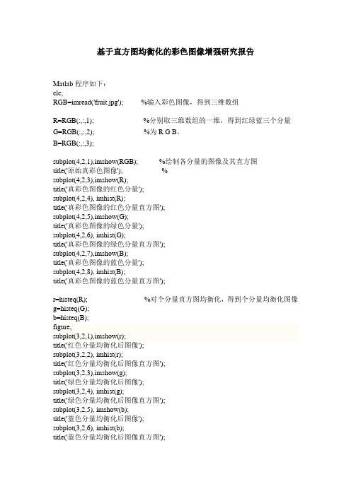
基于直方图均衡化的彩色图像增强研究报告Matlab程序如下:clc;RGB=imread('fruit.jpg'); %输入彩色图像,得到三维数组R=RGB(:,:,1); %分别取三维数组的一维,得到红绿蓝三个分量G=RGB(:,:,2); %为R G B。
B=RGB(:,:,3);subplot(4,2,1),imshow(RGB); %绘制各分量的图像及其直方图title('原始真彩色图像'); %subplot(4,2,3),imshow(R);title('真彩色图像的红色分量');subplot(4,2,4), imhist(R);title('真彩色图像的红色分量直方图');subplot(4,2,5),imshow(G);title('真彩色图像的绿色分量');subplot(4,2,6), imhist(G);title('真彩色图像的绿色分量直方图');subplot(4,2,7),imshow(B);title('真彩色图像的蓝色分量');subplot(4,2,8), imhist(B);title('真彩色图像的蓝色分量直方图');r=histeq(R); %对个分量直方图均衡化,得到个分量均衡化图像g=histeq(G);b=histeq(B);figure,subplot(3,2,1),imshow(r);title('红色分量均衡化后图像');subplot(3,2,2), imhist(r);title('红色分量均衡化后图像直方图');subplot(3,2,3),imshow(g);title('绿色分量均衡化后图像');subplot(3,2,4), imhist(g);title('绿色分量均衡化后图像直方图');subplot(3,2,5), imshow(b);title('蓝色分量均衡化后图像');subplot(3,2,6), imhist(b);title('蓝色分量均衡化后图像直方图');figure, %通过均衡化后的图像还原输出原图像newimg = cat(3,r,g,b); %imshow(newimg,[]);title('均衡化后分量图像还原输出原图');程序运行结果:通过matlab仿真,比较均衡化后的还原图像与输入原始真彩色图像,输出图像轮廓更清晰,亮度明显增强。
基于matlab的直方图均衡化
目录1、引言 (2)2、直方图基础 (3)3、直方图均衡化 (3)3.1 直方图均衡化的概念 (3)3.2 直方图均衡化理论 (4)3.3 Matlab 实现 (4)4、结论 (7)致谢 (7)参考文献 (7)图像增强处理—直方图均衡化的Matlab 实现摘要:为了使图像的灰度范围拉开或使灰度均匀分布,从而增大反差,使图像细节清晰,以达到增强的目的,通常采用直方图均衡化及直方图规定化两种变换,此文中探讨了直方图的理论基础,直方图均衡化的概念及理论,以Matlab为平台,对某地区遥感TM单波段遥感影像进行直方图均衡化,并给出了具体程序、仿真结果图像、直方图及变换函数。
实验结果表明,原来偏暗的且对比度较低的图像经过直方图均衡化后图像的对比度及平均亮度明显提高,直方图均衡化处理能有效改善灰度图像的对比度差和灰度动态范围。
关键词:图像增强直方图均衡化 Matlab1、引言图像增强是指对图像的某些特征,如边缘、轮廓或对比度等进行强调或尖锐化。
当一幅图像曝光不足或过度,造成对比度过小或过大而不能显示具体细节,通过增加这些细节的动态范围改善图像的视觉效果。
图像增强可以突出图像中所感兴趣的特征信息,改善图像的主观视觉质量,提高图像的可懂度。
增强的首要目标是处理图像,使其比原始图像更适合于特定应用。
图像增强的方法分为两大类:空间域方法和频域方法。
“空间域”一词是指图像平面本身,这类方法是以对图像的像素直接处理为基础的。
“频域”处理技术是以修改图像的傅氏变换为基础的。
一般说来,原始遥感数据的灰度值范围都比较窄,这个范围通常比显示器的显示范围小的多。
增强处理可将其灰度范围拉伸到0-255 的灰度级之间来显示,从而使图像对比度提高,质量改善。
增强主要以图像的灰度直方图最为分析处理的基础。
直方图均衡化能够增强整个图像的对比度,提高图像的辨析程度,算法简单,增强效果好。
本文主要讨论了空间域的直方图均衡化增强,并用Matlab 进行实验验证。
直方图均衡化matlab程序
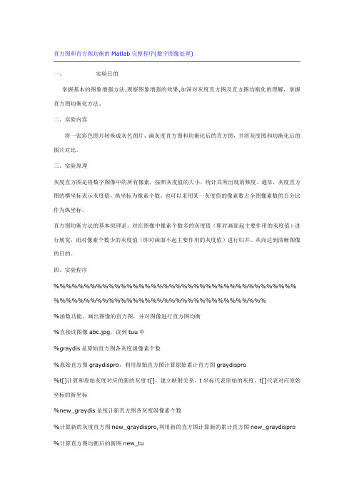
直方图和直方图均衡的Matlab完整程序(数字图像处理)一、实验目的掌握基本的图象增强方法,观察图象增强的效果,加深对灰度直方图及直方图均衡化的理解,掌握直方图均衡化方法。
二、实验内容将一张彩色图片转换成灰色图片,画灰度直方图和均衡化后的直方图,并将灰度图和均衡化后的图片对比。
三、实验原理灰度直方图是将数字图像中的所有像素,按照灰度值的大小,统计其所出现的频度。
通常,灰度直方图的横坐标表示灰度值,纵坐标为像素个数,也可以采用某一灰度值的像素数占全图像素数的百分比作为纵坐标。
直方图均衡方法的基本原理是:对在图像中像素个数多的灰度值(即对画面起主要作用的灰度值)进行展宽,而对像素个数少的灰度值(即对画面不起主要作用的灰度值)进行归并。
从而达到清晰图像的目的。
四、实验程序%%%%%%%%%%%%%%%%%%%%%%%%%%%%%%%%%%%%%%%% %%%%%%%%%%%%%%%%%%%%%%%%%%%%%%%%%%%%函数功能,画出图像的直方图,并对图像进行直方图均衡%直接读图像abc.jpg,读到tuu中%graydis是原始直方图各灰度级像素个数%原始直方图graydispro,利用原始直方图计算原始累计直方图graydispro%t[]计算和原始灰度对应的新的灰度t[],建立映射关系,t坐标代表原始的灰度,t[]代表对应原始坐标的新坐标%new_graydis是统计新直方图各灰度级像素个数%计算新的灰度直方图new_graydispro,利用新的直方图计算新的累计直方图new_graydispro %计算直方图均衡后的新图new_tu%%%%%%%%%%%%%%%%%%%%%%%%%%%%%%%%%%%%%%%% %%%%%%%%%%%%%%%%%%%%%%%%%%%%%%%%%%%clear allclose alltuu=imread('abc.jpg');%读入图片tu=rgb2gray(tuu);%将彩色图片转换为灰度图graydis=zeros(1,256);%设置矩阵大小graydispro=zeros(1,256);new_graydis=zeros(1,256);new_graydispro=zeros(1,256);[h w]=size(tu);new_tu=zeros(h,w);%计算原始直方图各灰度级像素个数graydisfor x=1:hfor y=1:wgraydis(1,tu(x,y))=graydis(1,tu(x,y))+1;endend%计算原始直方图graydisprograydispro=graydis./sum(graydis);subplot(1,2,1);plot(graydispro);title('灰度直方图');xlabel('灰度值');ylabel('像素的概率密度');%计算原始累计直方图for i=2:256graydispro(1,i)=graydispro(1,i)+graydispro(1,i-1);end%计算和原始灰度对应的新的灰度t[],建立映射关系for i=1:256t(1,i)=floor(254*graydispro(1,i)+0.5);end%统计新直方图各灰度级像素个数new_graydisfor i=1:256new_graydis(1,t(1,i)+1)=new_graydis(1,t(1,i)+1)+graydis(1,i); end%计算新的灰度直方图new_graydispronew_graydispro=new_graydis./sum(new_graydis);subplot(1,2,2);plot(new_graydispro);title('均衡化后的灰度直方图');xlabel('灰度值');ylabel('像素的概率密度');%计算直方图均衡后的新图new_tufor x=1:hfor y=1:wnew_tu(x,y)=t(1,tu(x,y));endendfigure,imshow(tu,[]);title('原图');figure,imshow(new_tu,[]);title('直方图均衡化后的图');//////////////////////////////////////////////////////另外两种代码:代码Matlab下面的代码来自archiless,注释非常详细,适合初学。
Matlab中的图像增强方法

Matlab中的图像增强方法图像增强是数字图像处理中的一项重要技术,通过使用各种算法和方法,可以改善图像的质量、增加图像的信息量和清晰度。
在Matlab中,有许多强大而灵活的工具和函数,可以帮助我们实现图像增强的目标。
本文将介绍几种常用的Matlab图像增强方法,并探讨它们的原理和应用。
一、直方图均衡化直方图均衡化是一种常用的图像增强方法,通过调整图像的像素分布来增强图像的对比度和亮度。
在Matlab中,我们可以使用“histeq”函数来实现直方图均衡化。
该函数会根据图像的直方图信息,将像素的灰度值重新映射到一个均匀分布的直方图上。
直方图均衡化的原理是基于图像的累积分布函数(CDF)的变换。
它首先计算图像的灰度直方图,并根据直方图信息计算CDF。
然后,通过将CDF线性映射到期望的均匀分布上,将图像的像素值进行调整。
直方图均衡化的优点在于简单易实现,且效果较好。
但它也存在一些限制,比如对噪声敏感、全局亮度调整可能导致细节丢失等。
因此,在具体应用中,我们需要权衡其优缺点,并根据图像的特点选择合适的方法。
二、自适应直方图均衡化自适应直方图均衡化是对传统直方图均衡化的改进,它能够在改善对比度的同时,保持局部细节。
与全局直方图均衡化不同,自适应直方图均衡化采用局部的直方图信息来进行均衡化。
在Matlab中,我们可以使用“adapthisteq”函数来实现自适应直方图均衡化。
该函数会将图像分成小块,并在每个块上进行直方图均衡化。
通过这种方式,自适应直方图均衡化可以在增强图像对比度的同时,保留图像的细节。
自适应直方图均衡化的优点在于针对每个小块进行处理,能够更精确地调整局部对比度,避免了全局调整可能带来的细节丢失。
然而,相对于全局直方图均衡化,自适应直方图均衡化的计算量较大,因此在实时处理中可能会引起性能问题。
三、模糊与锐化图像增强不仅局限于对比度和亮度的调整,还可以改善图像的清晰度和边缘信息。
在Matlab中,我们可以使用一些滤波器来实现图像的模糊和锐化。
基于matlab的图像对比度增强处理的算法的研究与实现
基于matlab的图像对比度增强处理的算法的研究与实现1. 引言1.1 研究背景图像对比度增强是数字图像处理中的一个重要领域,它能够提高图像的视觉质量,使图像更加清晰、鲜明。
随着现代科技的快速发展,图像在各个领域的应用越来越广泛,因此对图像进行对比度增强处理的需求也越来越迫切。
在数字图像处理领域,图像对比度增强处理是一种经典的技术,通过调整图像的灰度级范围,提高图像的对比度,使图像更加清晰和易于观察。
对比度增强处理可以应用于医学影像、卫星图像、照片修复等领域,有效提升图像质量和信息量。
随着数字图像处理算法的不断发展和完善,基于matlab的图像对比度增强处理算法也得到了广泛研究和应用。
通过matlab编程实现图像对比度增强处理算法,可以快速、高效地对图像进行处理,并进行实验验证和效果分析。
研究基于matlab的图像对比度增强处理算法的研究与实现具有重要的理论意义和实际应用价值。
1.2 研究目的研究目的是探索基于matlab的图像对比度增强处理算法,通过对比不同算法的效果和性能进行分析,进一步提高图像的清晰度和质量。
具体目的包括:1. 深入理解图像对比度增强处理的基本原理,掌握常用的算法和技术;2. 研究基于matlab的图像对比度增强处理算法实现的方法和步骤,探究其在实际应用中的优劣势;3. 通过实验结果与分析,评估不同算法在提升图像对比度方面的效果和效率;4. 对现有算法进行优化与改进,提出更加有效的图像对比度增强处理方法;5.总结研究成果,为今后进一步完善图像处理技术提供参考和借鉴。
通过对图像对比度增强处理算法的研究与实现,旨在提高图像处理的效率和质量,满足不同应用领域对图像处理的需求,促进图像处理技术的发展和应用。
1.3 研究意义对比度增强处理是图像处理领域中一项重要的技术,在实际应用中有着广泛的使用。
通过增强图像的对比度,可以使图像更加清晰、鲜明,提高图像的质量和观感效果。
对比度增强处理在医学影像分析、卫星图像处理、数字摄影等领域都有着重要的应用。
matlab的histeq函数
matlab的histeq函数
Matlab的histeq函数是一种直方图均衡化方法,通过将图像的像素
值重新分布来增强图像的对比度和亮度。
它可以用于改善图像的质量,使其更易于分析和处理。
在使用histeq函数之前,需要对图像进行预处理,将其转换为灰度图像。
然后,可以使用以下代码调用histeq函数:
```
I = imread('image.jpg'); % 读取图像
gray = rgb2gray(I); % 转换为灰度图像
J = histeq(gray); % 对灰度图像进行直方图均衡化
```
这段代码首先使用imread函数读取一张图像,然后使用rgb2gray函数将其转换为灰度图像。
最后,使用histeq函数对灰度图像进行直方图均衡化,并将结果保存在J中。
histeq函数的实现基于以下两个步骤:
1. 计算图像的直方图。
直方图是一种描述像素值分布的图表,它统计
了每个像素值出现的次数。
2. 重新分布像素值。
根据直方图信息,将像素值重新分布,使其更加均匀分布,从而增强图像的对比度和亮度。
在实际应用中,histeq函数可以用于图像增强、图像比较、色彩显著性分析等领域。
例如,在医疗图像中,直方图均衡化可以使图像的细节更明显,从而更易于诊断。
需要注意的是,histeq函数可能会导致图像出现过度增强和失真。
因此,在使用histeq函数之前,应该先对图像进行适当的调整,以确保结果符合需要。
总之,Matlab的histeq函数是一个常用的图像处理工具,可以帮助我们快速、方便地增强图像的对比度和亮度,提高图像的质量和可分析性。
MATLAB直方图均衡化代码(MATLABhistogramequalizationcode)

MATLAB直方图均衡化代码(MATLAB histogram equalization code)Im = imread (' c: \ 1. JPG); The % file is called 1.jpg image, which is in the bottom of c disk, and of course the path can be changed by itselfIf size (im, 3) > 1 % determines if it is color image, convert to grayscaleIm = rgb2gray (im);Endhist_im = imhist (im); % computing hist_im; % draw histogram Close allI = imread (' C: \ Documents and Settings \ DMT \ desktop \ intern \ image \ gray image \ lenna.bmp ')Imshow (I);Imhist (I);The Matlab complete program of histogram and histogram equalization is 2010-06-04 15:43:10Classification:I. experimental purposeGrasp the basic image enhancement method, observe the effect of image enhancement, deepen the understanding of grayscale histogram and histogram equalization, and master the method ofhistogram equalization.Second, experimental contentConvert a color image into a gray image, paint grayscale histogram and equalization of the histogram, and compare the grayscale to the equalization.Third, the experimental principleThe grayscale histogram is to calculate the frequency of all pixels in the digital image according to the size of the gray value. Generally, the horizontal coordinates of the grayscale histogram indicate the gray value, the ordinate is the number of pixels, or the pixel value of a certain gray value can be used as the vertical coordinate.The basic principle of histogram equalization method is that the number of pixels in the image of grey value (that is, a major role on the image grey value) for broadening, and a small number of pixels of grey value (that is, does not play a major role on the picture of the grey value) to carry on the merge. To achieve the purpose of clear image.4. Experimental procedure% % % % % % % % % % % % % % % % % % % % % % % % % % % % % % % % % % % % % % % % % % % % % % % % % % % % % % % % % % % % % % % % % % % % % % % % % % %Function of % function, draw the histogram of the image, andmake histogram equalization to the image% direct read ABC. JPG, read to tuu% graydis is the number of grayscale pixels in the original histogram% primitive histogram graydispro, using the original histogram to calculate the original cumulative histogram graydisproThe new grayscale t [] calculated and the original grayscale corresponds to the new gray value t [], the mapping relationship is established, the t coordinates represent the original grayscale, and t [] represents the new coordinates corresponding to the original coordinates% new_graydis is the number of grayscale pixels of the new histogramThe new histogram new_graydispro is calculated and the new histogram new_graydispro is calculated using the new histogramThe new figure new_tu after the histogram equalization is calculated% % % % % % % % % % % % % % % % % % % % % % % % % % % % % % % % % % % % % % % % % % % % % % % % % % % % % % % % % % % % % % % % % % % % % % % % % % %Clear allClose allTuu = imread (' ABC. JPG); % read in picturesTu = rgb2gray (tuu); % converts color images to grayscaleGraydis = zeros (1256); % sets the matrix sizeGraydispro = zeros (1256);New_graydis = zeros (1256);New_graydispro = zeros (1256);H [w] = size (tu);New_tu = zeros (h, w);Graydis of grayscale pixels in the original histogram of the original histogramFor x = 1: hFor y = 1: wGraydis (1, tu (x, y)) = graydis (1, tu (x, y)) + 1;The endThe end% computing the original histogram graydisproGraydispro = graydis. / sum (graydis);Subplot (1, 2, 1);The plot (graydispro);Title (' grayscale histogram ');Xlabel (' gray value '); Ylabel (' pixel probability density ');Calculate the original cumulative histogram6 for I ="Graydispro (1, I) = graydispro (1, I) + graydispro (1, I - 1);The endThe new grayscale t [] with the corresponding % computation and the original grayscale is established to map the relationshipFor I = 25 JuneT (1, I) = floor (254 * graydispro (1, I) + 0.5);The end% statistics new histogram each grayscale pixel numbernew_graydisFor I = 25 JuneNew_graydis (1, t + 1) (1, I) = new_graydis (1, t (1, I) + 1) + graydis (1, I);The endCalculate the new grayscale histogram new_graydisproNew_graydispro = new_graydis. / sum (new_graydis);Subplot (1,2,2);The plot (new_graydispro);Title (" equalization of grayscale histogram ");Xlabel (' gray value '); Ylabel (' the probability density of pixels');The new figure new_tu after the histogram equalization is calculatedFor x = 1: hFor y = 1: wNew_tu (x, y) = t (1, tu (x, y));The endThe endFigure, imshow (tu, []);The title (' artwork ');Figure, imshow (new_tu, []);Title (' histogram equalization ');/ / / / / / / / / / / / / / / / / / / / / / / / / / / / / / / / / / / / / / / / / / / / / / / / / / / / / /The other two codes:codeMatlabThe following code is from archiless, which is very detailed and suitable for beginners.The % digital image processing program job% this program can grayscale and histogram equalization of JPG color image files%% input file: picsam.jpg for image processing% output file: PicSampleGray. BMP grayscale image% PicEqual. BMP equalization after image%% output graphical window descriptionThe color image is processed in % figure NO 1% figure NO 2 grayscale image% figure NO 3 histogram% figure NO 4 equalization of histogram% figure NO 5 greyscale% figure NO 6 equalization of the image% 1, the image you handle is picsam.jpg% 2, the program will clear the workspace every time it runs % the author; Archiless lorderClear all% 1, the image preprocessing, read into the color image to thegrayscalePS = imread (' PicSample. JPG);% read in JPG color image filesImshow (PS) % shows figure NO 1Title (' input color JPG image ')Imwrite (rgb2gray (PS), 'PicSampleGray. BMP); % color image grayscale and savePS = rgb2gray (PS); % grayscale data is stored in an arrayFigure, imshow (PS) % shows the grayscale image and the sample figure NO 2 before equalizationTitle (' grayscale image ')% 2 draw histogram[m, n] = size (PS); % measurement of image size parametersGP = zeros (1256); % precreate vectors that store probability of grayscaleFor k = 0:25 5GP (k + 1) = length (find (PS = = k))/(m * n); The probability of calculating the gray level of each level is calculated anddeposited into the corresponding position in the GPThe endFigure, bar (0:255, GP, 'g') % draw histogram figure NO 3 Title (' original image histogram ')Xlabel (' gray value ')Ylabel (' occurrence probability ')Third, the histogram equalizationS1 = zeros (1256);For I = 25 JuneFor j = 1: i.S1 (I) = GP (j) + S1 (I); % calculation SkThe endThe endS2 = round (S1 * 256); % return Sk to a similar level of grayscale For I = 25 JuneGPeq (I) = sum (GP (find (S2 = = I))); The probability of thepresent occurrence of each grayscale is calculatedThe endFigure, bar (0:25, GPeq, 'b') % display equalization of the histogram figure NO 4Title (histogram after equalization)Xlabel (' gray value ')Ylabel (' occurrence probability ')Figure, plot (0:25, S2, 'r') % display grayscale change curve figure NO 5Legend (' grayscale change curve ')Xlabel (' original image greyscale ')Ylabel (' post-equalization greyscale ')4. Image equalizationPA = PS;For I = 0:25 5PA (find (PS = = I)) = S2 (I + 1); % assigns each pixel to the pixel with a normalized gray valueThe endFigure, imshow (PA) % display equalization of the image figure NO 6Title (' equalized image ')Imwrite (PA, 'PicEqual. BMP);Another Matlab code, from histogram equalization - image enhancementI = imread (' LENA256. BMP);Imshow (I);Figure;Imhist (I);[m, n] = size (I);Hf = zeros (1256);Pa = zeros (1256);I = double (I);For I = 1: mFor j = 1: nHf (I + 1) (I, j) = hf (I (I, j) + 1) + 1; % statistics the number of grayscale pixelsThe endThe endBmap = zeros (1256);For I = 25 JuneTemp = 0;For j = 1: i.Temp = temp + hf (j);The endBmap (I) = floor (temp * 255 / (m * n));The endY = zeros (m, n);For I = 1: mFor j = 1: nY (I, j) = bmap (I (I, j) + 1);The endThe endY = uint8 (y);Figure;Imshow (y);Clear all;I = imread (' 1. JPG);I = rgb2gray (I); % gray,Make a histogram[m, n] = size (I);GP = zeros (1256);For k = 0:25 5GP (k + 1) = length (find) (I = = k)/(m * n); The probability of calculating the occurrence of grayscale at each level is deposited into GPThe endThird, the histogram equalizationS1 = zeros (1256);For I = 25 JuneFor j = 1: i.S1 (I) = GP (j) + S1 (I);The endThe endS2 = round (+ 0.5) * 256 (S1); % return Sk to a similar level of grayscaleFor I = 25 JuneGPeq (I) = sum (GP (find (S2 = = I))); The probability of the present occurrence of each grayscale is calculatedThe endFigure;Subplot (221); Bar (0:25 5, GP, 'b');Title (' original image histogram ')Subplot (222); Bar (0:25 5, GPeq, 'b')Title (histogram after equalization)X = I;For I = 0:25 5X (find (I = = I)) = S2 (I + 1);The endSubplot (223); Imshow (I);Title (' original image ');Subplot (224); Imshow (X);Title (' histogram equilibrium image ');。
- 1、下载文档前请自行甄别文档内容的完整性,平台不提供额外的编辑、内容补充、找答案等附加服务。
- 2、"仅部分预览"的文档,不可在线预览部分如存在完整性等问题,可反馈申请退款(可完整预览的文档不适用该条件!)。
- 3、如文档侵犯您的权益,请联系客服反馈,我们会尽快为您处理(人工客服工作时间:9:00-18:30)。
课程设计报告题目基于matlab的直方图均衡化程序设计学生姓名:学生学号:系别:专业:届别:指导教师:电气信息工程学院制目录1、引言·······················································································- 2 -2、直方图基础 ···············································································- 2 -3、直方图均衡化············································································- 3 -3.1 直方图均衡化的概念·····················································································- 3 -3.2 直方图均衡化理论························································································- 4 -3.3 Matlab 实现······························································································- 4 -4、结论 ······················································································- 10 -5、心得体会················································································- 10 -参考文献·····················································································- 10 -基于matlab的直方图均衡化程序设计指导老师:马立宪电气工程学院:电子信息工程摘要:为了使图像的灰度范围拉开或使灰度均匀分布,从而增大反差,使图像细节清晰,以达到增强的目的,通常采用直方图均衡化及直方图规定化两种变换,此文中探讨了直方图的理论基础,直方图均衡化的概念及理论,以Matlab 为平台,对某地区遥感TM单波段遥感影像进行直方图均衡化,并给出了具体程序、仿真结果图像、直方图及变换函数。