斯科特微观经济学课件Chapter 20 - Market entry and the emergence of perfect competition
合集下载
微观经济学-第一章及第二章PPT课件

Qd P
2020/3/28
22
二、需求规律
一般而言,某种商品的价格越高,消费者愿意并且能够购买的该商品 的数量就会越少;反之,价格越低,消费者愿意并且能够购买的该商品的 数量就越多。我们将这种需求量与价格的反方向变动规律称之为需求规律。
特例:
吉芬商品——需求曲线向右上方倾斜
2020/3/28
2020/3/28
33
第三节 市 场 均 衡
一、均衡、均衡价格与均衡数量
1、均衡的含义
均衡是指经济体系中一个特定的经济单位或者经济变量在一系列经济 力量的相互制约下所达到的一种相对静止并保持不变的状态。
供求力量的相互作用使得一个市场处于均衡状态,市场价格就趋于不 变。
2020/3/28
34
2、均衡价格与均衡数量
政策主张:自由放任
2020/3/28
5
三、新古典经济学:微观经济学的形成与建立时期 ( 19c70 年代 —20c30年代)
主要代表人物 :(奥)门格尔、(英)杰文斯
(法)瓦尔拉斯、(英)马歇尔
代表作: 《经济学原理》(1890) 马歇尔
基本观点 :从供给和需求两方面同时进行分析的均衡价格论,以边际效 应论来说明需求,一生产费用论来说明供给,由此形成均衡价格理论,用 价格理论来代替价值理论。
2020/3/28
9
二、西方经济学的研究对象 西方经济学的研究对象为资源的有效配置及合理利用
2020/3/28
10
第四节 西方经济学的研究方法
一、经济模型与数学分析 二、静态分析、比较静态分析与动态分析 三、实证分析与规范分析 四、边际分析
2020/3/28
11
第五节 如何看待西方经济学
2020/3/28
22
二、需求规律
一般而言,某种商品的价格越高,消费者愿意并且能够购买的该商品 的数量就会越少;反之,价格越低,消费者愿意并且能够购买的该商品的 数量就越多。我们将这种需求量与价格的反方向变动规律称之为需求规律。
特例:
吉芬商品——需求曲线向右上方倾斜
2020/3/28
2020/3/28
33
第三节 市 场 均 衡
一、均衡、均衡价格与均衡数量
1、均衡的含义
均衡是指经济体系中一个特定的经济单位或者经济变量在一系列经济 力量的相互制约下所达到的一种相对静止并保持不变的状态。
供求力量的相互作用使得一个市场处于均衡状态,市场价格就趋于不 变。
2020/3/28
34
2、均衡价格与均衡数量
政策主张:自由放任
2020/3/28
5
三、新古典经济学:微观经济学的形成与建立时期 ( 19c70 年代 —20c30年代)
主要代表人物 :(奥)门格尔、(英)杰文斯
(法)瓦尔拉斯、(英)马歇尔
代表作: 《经济学原理》(1890) 马歇尔
基本观点 :从供给和需求两方面同时进行分析的均衡价格论,以边际效 应论来说明需求,一生产费用论来说明供给,由此形成均衡价格理论,用 价格理论来代替价值理论。
2020/3/28
9
二、西方经济学的研究对象 西方经济学的研究对象为资源的有效配置及合理利用
2020/3/28
10
第四节 西方经济学的研究方法
一、经济模型与数学分析 二、静态分析、比较静态分析与动态分析 三、实证分析与规范分析 四、边际分析
2020/3/28
11
第五节 如何看待西方经济学
微观经济学ppt课件
在B点左侧TPL凸向右下方,在B
点右侧TPL凸向左上方。
O MP
L
当MPL>0时,ΔTPL>0;
当MPL<0时,ΔTPL<0 ;
B’
当MPL=0时,TPL最大 。
MPL D’
O
MPL L28/71
※总产量曲线与平均产量曲线的关系
Q
D
C
APL等于原点与TPL上任一
B
点连线的斜率。
APL最高点C′对应着TPL上
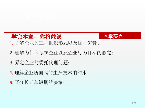
单业主制企业(sole properietorship) 合伙制企业(partnership) 公司制企业(cooperation)
4/71
一、单业主企业
单业主企业又称个人企业,是一个人拥有 并负责经营管理的企业组织形式。
优势:
由于规模小,易于管理,没有沉重的行政管理 及其费用的负担;
18/71
6.2.2决策的时间框架
短期(short-run)——在此期间内,至少有 一种投入的数量不变而其他投入的数量可 以变动。
短期内资本K的数量不能改变,即不能增加 机器设备等,而劳动L的数量则是可以改变
的,因此,Q短期f (生L产, K函) 数一般记为:
Q f (L)
19/71
6.2.2决策的时间框架
公司制企业实行法人治理结构,即形成由 股东大会、董事会、经理层和监事会组成 并有相互制衡关系的管理机制。
股份公司是一种两权分离的组织形式。
9/791
三、公司制企业
公司制企业的优势有:
筹资容易、公司是一种最为有效的融资组织形 式,它通过发行股票和债券,筹集社会公众的 闲散资金;
所有者承担有限责任 管理不受所有者能力限制、管理的专门化水平; 连续性强、不会因为总经理的死亡、辞退而
微观经济学英文课件

Edited by Yong, E.L.
Continuously,
Microeconomics is also used for evaluating broad question in regards to government policy (although this is more to macroeconomics).
Edited by Yong, E.L.
Continuously,
If the firm produces 6 units of apple and 12 units of apple pie wants to increase the production of apple pie by one unit to the 13th unit. It has to forgo 2 units of apple so that resources can be shifted to produce the additional apple pie; Opportunity Cost is thus 2.
Edited by Yong, E.L.
Continuously,
If the firm produces 10 units of apple and 6 units of apple pie wants to increase the production of apple pie by one unit to the 7th unit. It has to forgo 1 unit of apple so that resources can be shifted to produce the additional apple pie; Opportunity Cost is thus 1.
微观经济学概述PPT课件

12
(2)古典经济学革命
《国富论》的出版被称为经济学史上的第 一次革命,即古典经济学革命。其标志着微观 经济的诞生,以斯密为代表的古典经济学的贡 献是建立了以自由放任的市场经济为中心的经 济学体系。
13
古典经济学自由放任的思想反映了自由 竞争时期经济发展的要求。古典经济学家把经 济研究从流通领域转移到生产领域,使经济学 真正成为有独立体系的学科。
31
1.动态分析
动态分析则对经济变动的实际过程进行 分析,其中包括分析有关的经济总量在一定时 间过程中的变动,这些经济总量在变动过程中 的相互影响和彼此制约的关系,以及它们在每 一时点上变动的速率等等。这种分析考察时间 因素的影响,并把经济现象的变化当作一个连 续的过程来看待。
32
三、边际分析方法
一、微观经济学发展简况 二、微观经济学及其体系
9
一、微观经济学发展简况
1.古典经济学时期——微观经济学的形成时期 2.新古典经济学时期——微观经济学的建立时期
10
1.古典经济学时期
(1)对古典经济学的说明 (2)古典经济学革命
11
(1)对古典经济学的说明
我们这里所说的古典经济学是从17世纪 中期开始,到19世纪70年代前为止,其代表人 物包括英国经济学家亚当•斯密、大卫•李嘉图、 西尼尔、约翰•缪勒、马尔萨斯。其中最重要 的代表人物是亚当•斯密,其代表作是1776年 出版的《国富论》
管理者必须学会告别过去的失误,做到 立足于现实,面向未来地进行决策。
37
3.边际分析方法的深化
边际分析法要求正确处理好增量与存量的 关系
(1)通过增量,激活存量,实现总量的共同 发展。
(2)控制增量,而盘活存量。
38
微观经济学导论
《微观经济学》课件2

利润最大化原则的应用
03
企业在制定生产计划时,应遵循利润最大化原则,以实现企业
利润的最大化。
05
CATALOGUE
市场结构理论
市场结构的类型
寡头市场
寡头市场是指市场上只有少数几家大企业 ,这些大企业共同控制了市场价格和产量 。
市场结构的类型
市场结构主要分为四种类型,包括完全竞 争市场、垄断市场、垄断竞争市场和寡头 市场。
政府可以通过反垄断政策来限制垄断行为,保护市场竞争。
政府管制
政府可以对某些行业或企业进行管制,以保护消费者利益和社会公共利益。
THANKS
感谢观看
完全竞争市场的特点
完全竞争市场具有以下特点,包括产 品同质、信息完全、进出自由和众多 小规模企业。
完全竞争市场的均衡
在完全竞争市场上,企业只能被动接 受市场价格,达到均衡状态时,企业 的产量是由边际成本等于边际收益决 定的。
垄断市场
垄断市场的特点
垄断市场具有以下特点,包括独 家企业、产品独占、实行差别价 格、存在进入障碍。
边际效用理论
边际效用理论是消费者行为理论的重要组成部分,它解释了消费者如何根 据商品的边际效用来做出购买决策。
商品的边际效用表示消费者在增加或减少一单位商品消费时所获得的效用 增量。
根据边际效用递减规律,随着消费者对某一种商品消费的增加,该商品的 边际效用会逐渐减少。
消费者均衡
01
消费者均衡是消费者在有限的收入和商品价格下所达到的 最优消费状态。
03
CATALOGUE
消费者行为理论
消费者行为模型
1
消费者行为模型是微观经济学中的一个基本模型 ,它描述了消费者如何在有限的收入和商品价格 下做出最优的消费决策。
《微观经济学microeconomics》英文版全套课件(101页)

X RL {x R : xl 0 for l 1,..., L}
The economic constraint:
px p1x1 ... pL xL w
The Walrasian budget set (Definition 2.D.1)
Bp,w {x RL : px w}
or
u(x* ) xl
pl
px w
Solution: Walrasian demand function x*( p, w)
Utility Maximization -- Example
Example 3.D.1: the transformed Cobb-Douglas Utility Function
Expenditure Function
Expenditure function e( p,u) Min px s.t. u(x) u {x}
Properties: 1. Homogeneous of degree of one in p 2. Strictly increasing in u and nondecreasing in p 3. Concave in p 4. Continuous in p and u
Comparative Statics – Wealth Effects
The consumer’s Engel function x( p, w)
The wealth effect xl ( p, w) / w or Dwx( p, w) Normal goods and inferior goods
A choice rule C(B) B
The weak axiom of revealed preference (WARP): if x is revealed at least as good as y, then y cannot be revealed preferred to x
微观经济学英文版ppt课件ch20checkpoint
The demand curve for managers and professionals, DH, is greater than the demand for salespeople, DL.
CHECKPOINT 20.2
The figure shows that the combination of demand and supply leads to a higher wage rate for managers and professionals than for salespeople.
CHECKPOINT 20.1
Solution
A Lorenz curve plots the cumulative percentage of income against the cumulative percentage of households.
The blue curve plots the data for the Canadian Lorenz curve.
The green curve plots the data for the U.S. Lorenz curve.
CHECKPOINT 20.1
The line of equality shows an equal distribution.
The Canadian Lorenz curve lies closer to the line of equality than the U.S. Lorenz curve, so the distribution of income in the United States is more unequal than that in Canada.
微观经济学完整版(获奖课件)
无差异曲线与预算线的切点
代表消费者在该预算约束下能够达到的最大效用水平,即 最优消费组合。
消费者均衡与需求曲线的推导
要点一
消费者均衡
在既定的收入和商品价格下,消费者 选择最优的商品组合使得总效用最大 化。此时,无差异曲线与预算线相切 。
要点二
需求曲线的推导
基于消费者均衡条件,可以推导出消 费者对某种商品的需求曲线。随着商 品价格的变化,消费者的最优选择也 会发生变化,从而得到不同价格下的 需求量。将这些点连接起来,便得到 需求曲线。
相互联系
微观经济学和宏观经济学是相互联系的,微观经济学的理论和方法可以为宏观经济学提供 基础和支持,同时宏观经济学的理论和方法也可以为微观经济学提供指导和借鉴。两者共 同构成了经济学的完整体系。
02
需求、供给与均衡价格
需求理论
01
02
03
需求函数
描述商品需求量与其价格 之间的关系,通常需求量 与价格呈反方向变动。
要素供给
要素供给取决于要素所有者的偏 好、财富状况以及要素价格。一 般而言,要素价格越高,要素供 给量就越大。
要素市场的均衡
在要素市场上,要素需求和供给 相互作用,最终决定要素的均衡 价格和均衡数量。
工资、利息、地租和利润的决定
工资的决定
利息的决定
工资是劳动的报酬,其水平取决于劳动市 场的供求状况、劳动生产率、劳动力素质 以及社会经济发展水平等因素。
价格管制对市场均衡的影响
价格管制会打破市场均衡,导致资源配置效率降 低。长期实施价格管制还可能影响市场供求关系 ,造成市场扭曲。
税收政策及其影响分析
税收种类
包括所得税、消费税、财产税等,不同税种对微观经济主体行为产生不同影响。
斯科特微观经济学课件Introduction
8/10/2021
25
经济学演变图谱
魁奈 1758
重农学派
亚当·斯密 1776
托马斯 ·曼
古典经济学
重商主义 15-17
社会主义 马克思1867 列宁1917
中国
李嘉图 1817
马尔萨斯 1798
J.S穆勒 1848
前苏联、 东欧国家
转轨经济
凯恩斯 1936
新古典经济学
瓦尔拉 马歇尔 费雪 1880-1910
31
小结
1.Adam smith →Marshall →Keynes →… 2.Scarcity→Choice→Opportunity cost 3.Production Possibilities Frontier 4.Micro Vs. Macro 5.Positive Vs. Normative
或PPC曲线)生产可能性边界也称生产可能性曲线或产
品转换曲线(product transformation curve) 。
8/10/2021
15
一定技术和资源条件下,两 种产品最大产量的组合如表
组合 民用品
军用品
A M NB 10 9 5 0
0 3 59
民 用 品A
MC
生产可能 性边界
N E
D
• Efficiency(D→E) • Tradeoffs (M→N)
8/10/2021
7
一、为什么要学经济学?
一个社会的兴衰在某种程度上取决于其政 府所选择的公共政策;理解、赞成或反对 某项政策的各种意见是我们研究经济学的 一个理由。
各国领导人(政治家):制定经济政策 经济学家:解释整个经济如何运行 有助于理性地作决策
西方经济学---微观部分-----第一章--市场-Ch01-The-MarketPPT课件
Market Demand Curve for Apartments
p
QD
Modeling Apartment Supply
• Supply: It takes time to build more close apartments so in this short-run the quantity available is fixed (at say 100).
Modeling Apartment Demand
• Demand: Suppose the most any one
person is willing to pay to rent a close
apartment is $500/month. Then
p
= $500 QD = 1.
• Suppose the price has to drop to $490 before a 2nd person would rent. Then p
p
People willing to pay pe for close apartments get close apartments.
pe 100
QD,QS
Competitive Market Equilibrium
p
People willing to pay pe for close apartments get close apartments.
Market Supply Curve for Apartments
p
100
QS
Competitive Market Equilibrium
• “low” rental price quantity demanded of close apartments exceeds quantity available price will rise.
- 1、下载文档前请自行甄别文档内容的完整性,平台不提供额外的编辑、内容补充、找答案等附加服务。
- 2、"仅部分预览"的文档,不可在线预览部分如存在完整性等问题,可反馈申请退款(可完整预览的文档不适用该条件!)。
- 3、如文档侵犯您的权益,请联系客服反馈,我们会尽快为您处理(人工客服工作时间:9:00-18:30)。
• Equilibrium - not subgame perfect equilibrium
• Monopolist
– Keep same output level
• Not best choice – If new firms enter
12
Figure 20.6
The entry-prevention game
– Incumbent firm - deter entry
• Policy - best for monopolist
5
Figure 20.2
Residual demand for the potential entrant: a case of blockaded entry
Price MC AC Once the incumbent firm has set its output level at qm, the potential entrant faces a residual demand curve of p= (A-bqm)-bqe. In this case, because the average cost curve is above the demand curve for all output levels, profitable entry is impossible.
v+s
v
0
K
Output
18
Entry Prevention, Overinvestment, and the Dixit-Spence Model
• Overinvestment strategy
– Entry-prevention strategy – Incumbent monopolist
11
pe
Criticisms of the Bain, Modigliani, Sylos-Labini Model: Subgame Perfection
• Bain, Modigliani, Sylos-Labini model
– Limit-pricing strategy for entry prevention – Game theory
• Limit pricing
– Established firms
• Deter entry
• Set output
• Remaining demand – too low – New entrants – no profit
3
Figure 20.1
Limit pricing: Bain, Modigliani, Sylos-Labini model
32 0
36 0
32 0
ห้องสมุดไป่ตู้28 0
32 0
28 0
Backward induction leads to high output in period 1, entry, and both firms’ choosing M in the last stage
Entry Prevention, Overinvestment, and the Dixit-Spence Model
4
Limit Pricing
• Residual demand curve
– Demand curve
• Remaining demand for potential entrant • After: incumbent firm - set its output
• Blockaded entry
• Dixit-Spence model
– Model of entry prevention – Incumbent monopolist
• Overinvest in production capacity • Entry – unprofitable
16
Entry Prevention, Overinvestment, and the Dixit-Spence Model
pe
MR 0
qe
D
Quantity (qe)
6
Impeding Market Entry
• Impeded entry
– Monopolist
• Sets - less advantageous level of output • To deter entry – New firms into market
• Production capacity – K
– If output < K (excess capacity)
• Marginal cost = v
– If output > K (no excess capacity)
• Marginal cost = v+s
17
Figure 20.8
Marginal cost function for a capacity-constrained firm
14
Figure 20.7
The Donut game
H M Mrs. Donut L Freddie’s In
Out
In
Out
In
Out
Play entry game
H
M L
Play entry game
H
M
L
Play entry game
H
Mrs. Donut M
L
24 0
15
40 0
36 0
Criticisms of the Bain, Modigliani, Sylos-Labini Model: Subgame Perfection
• No subgame perfect equilibrium
– If new entry – Rational incumbent
• First period – Output – Monopoly price – Maximize profits • Next period – Abandon output set in first period
Marginal cost At output levels that are lower than the firm’s installed capacity of K, the marginal cost is merely the variable marginal cost of ν. At higher output levels, the marginal cost also includes the cost of additional capacity, s.
– Block entry – Otherwise: lower profits
2
Limit Pricing
• Bain, Modigliani, Sylos-Labini model
– Incumbent firm - pricing strategy
• Unprofitable - potential competitors
• Cost function – incumbent monopolist
if q K vq F , Ci(q, K ) vq s(q K ), if q K
• Impede entry
10
Figure 20.5
The residual demand for the potential entrant: a case of impeded entry
Price
MC A-bqL AC Instead of setting the monopoly quantity of qm and the monopoly price of pm, the incumbent firm sets the limit quantity of qL and the limit price of pL. This lowers the residual demand curve so that it is tangent to the potential entrant’s average cost curve, making profitable entry impossible. MR 0 qe D Quantity (qe)
1
Set output of q Incumbent Set output of q qL
Potential Entrant
Enter market Incumbent Keep output q= q 3
qm
2
Don’t Enter market
Potential Entrant
The incumbent firm moves first by choosing a quantity level in the set (q, q). The entrant then moves by choosing either to enter the market or to stay out. Finally, the incumbent firm moves by choosing its best response to the entrant’s output level.
Chapter 20
Market Entry and the Emergence of Perfect Competition
Need for Entry-Prevention Strategies
• Monopolist – extra-normal profit • Other firms – want to enter the market • Monopolist