计量经济学
计量经济学概念

第二节 计量经济学方法
一. 计量经济学方法的内容
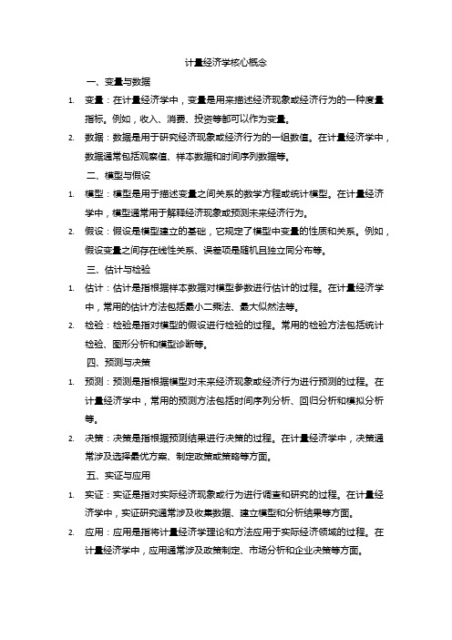
任何计量经济研究包含两个基本要素:理论和事实, 计量经济学的主要功能就是将这两个要素结合在一起。 计量经济研究既使用理论,也使用事实,将二者结合 起来,用统计技术估计经济关系,如图1.1所示。
14
理论统计理论
计量经济模型
加工好的数据
10
3. 学科发展环境 同时,随着科学技术的发展,各门学科相互渗透,数
学、系统论、信息论、控制论等相继进入经济研究领 域,使经济科学进一步数量化,有助于计量经济学的 发展。高速电子计算机的出现和发展,为计量经济技 术的广泛应用铺平了道路。
11
4. 发展过程
上世纪三十年代,侧重于个别商品供给与需求的计 量,基本上属于个量分析或微观分析。
1. 需求函数的数学模型
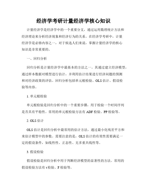
尽管需求定律假定价格(P)与需求量(Q)之间 呈反向关系,但并没有给出二者之间关系的精 确形式。例如,该定律并没有告诉我们价格与 需求量之间关系是线性的还是非线性的,如图 1.2中(a)和 (b) 所示。
21
Q
Q
(a)
P
(b)
P
图1.2 线性和非线性的需求函数
22
事实上,斜率为负的曲线有千千万万,在它们 之中选择正确的函数是计量经济学家的任务。
7
计量经济学的艺术成分
计量经济学虽然以科学原理为基础,但仍保留了一 定的艺术成分,主要体现在试图找出一组合适的假设 ,这些假设既严格又现实,使得我们能够使用可获得 的数据得到最理想的结果,而现实中这种严格的假设 条件往往难以满足。
“艺术”成分的存在使得计量经济学有别于传统 的科学,是使人对它提供准确预测的能力产生怀疑的 主要原因。
31
计量经济学

计量经济学计量经济学,是一门使用统计方法分析经济现象的学科。
计量经济学主要通过收集、处理、分析和解释经济数据,以确认和识别经济核心问题,比如需求和供给、价格变动、市场结构和经济增长等。
这门学科的进步和应用在各种政策制定和经济决策上有着广泛的应用领域,比如经济政策的分析,股票市场的预测和企业的经营决策等。
接下来,本文将解释计量经济学的主要内容和方法,并探讨计量经济学在实践中的应用。
一、计量经济学的主要内容计量经济学分析的主要对象是经济现象和经济数据。
这些现象和数据可以描述为变量和关系,比如价格,工资,利润和经济增长等。
计量经济学主要研究的是这些变量及其之间的相互关系,以便为决策者提供更好的政策建议。
在计量经济学中,通常会涉及到如下的主要内容:1. 变量的含义和测量。
计量经济学要求研究者对变量的含义进行明确界定,以便能够对其进行测量,并进行数据收集和分析。
例如,如果要研究通货膨胀的影响因素,通货膨胀就是一个重要的变量,需要进行合理的测量。
2. 经济关系的建模。
计量经济学则进一步探索变量之间的数量关系,并通过数学模型来描述它们之间的联系。
例如,经济学家可以建立一个供求模型来研究商品价格的形成。
3. 假设检验。
计量经济学通过提出假设并使用统计检验方法来验证假设。
通过检验结果,经济学家可以同样的推理得出各种假设是否成立。
4. 统计分析。
该领域强调通过统计分析方法检验模型的假设,这是检验数据和变量关系的重要手段。
统计分析包括回归分析、时间序列分析以及多元统计分析等方法。
二、计量经济学方法计量经济学的重要方法包括统计分析、回归分析、时间序列分析、概率论和经济实验等。
其中最常使用的方法是回归分析。
1. 回归分析回归分析是计量经济学的核心方法。
回归分析将一个自变量与因变量相关联。
例如,如果我们想知道变量X与变量Y的相关性,我们就会回归一个X对Y的方程。
这个方程告诉我们,当X发生变化时,Y的变化程度。
回归分析需要建立方程,并根据现有数据的信息来确定系数。
计量经济学名词解释

计量经济学名词解释1、计量经济学计量经济学是一个分支学科,以揭示经济活动中客观存在的数量关系为内容的分支学科,统计学,经济理论和数学这结合便构成了计量经济学。
2、计量经济学模型揭示经济活动中各个因素之间的定量关系,用随机性的数学方程加以描述。
3、解释变量影响被解释变量的因素或因子,是原因变量,记为“X”.4、被解释变量结果变量称为被解释变量,记为“Y”。
5、结构分析结构分析是对经济现象中变量之间相互关系的研究。
所采用的主要方法是弹性分析、乘数分析与比较静力分析。
6、时间序列数据按照时间先后顺序排列的统计数据,又称为纵向数据。
7、截面数据一批发生在同一时间截面上的调查数据,又称横向数据。
8、平行数据(面板数据)时间序列数据与截面数据的合成体,又称面板数据。
9、回归分析回归分析是研究一个变量关于另一个(些)变量的依赖关系的计算方法和理论。
10、随机误差项被解释变量数值与其条件期望之间的离差,是一个不可观测的随机变量,称为随机误差项,或随机干扰项。
11、最小二乘法通过最小化误差的平方和寻找数据的最佳函数匹配。
12、最佳线性无偏估计量拥有有限样本性质或小样本性质这类性质的估计量,称为最佳线性无偏估计量。
13、拟合优度是SRF对样本观测值的拟合程度,即样本回归直线与观测散点之间的紧密程度。
14、方程显著性检验对所有被解释变量与解释变量之间的线性关系在总体上是否显著成立做出推断的检验。
15、变量显著性检验是对模型中某一个具体的解释变量X与被解释变量Y之间的线性关系在总体上是否显著成立做出判断,换言之,是考察所选择的X在总体上是否对Y有显著的线性影响。
16、最小样本容量是指从最小二乘原理和最大似然原理出发,欲得到参数估计量,不管其质量如何,所要求的样本容量的下限。
17、满足基本要求的样本容量当n≥30或者至少n≥3(k+1)时,才能说满足模型估计的基本要求。
18、需求函数的零阶齐次性当所有商品价格和消费者货币支出总额按照同一比例变动时,需求量保持不变,这就是所谓的消费者无货币幻觉。
计量经济学核心概念
计量经济学核心概念一、变量与数据1.变量:在计量经济学中,变量是用来描述经济现象或经济行为的一种度量指标。
例如,收入、消费、投资等都可以作为变量。
2.数据:数据是用于研究经济现象或经济行为的一组数值。
在计量经济学中,数据通常包括观察值、样本数据和时间序列数据等。
二、模型与假设1.模型:模型是用于描述变量之间关系的数学方程或统计模型。
在计量经济学中,模型通常用于解释经济现象或预测未来经济行为。
2.假设:假设是模型建立的基础,它规定了模型中变量的性质和关系。
例如,假设变量之间存在线性关系、误差项是随机且独立同分布等。
三、估计与检验1.估计:估计是指根据样本数据对模型参数进行估计的过程。
在计量经济学中,常用的估计方法包括最小二乘法、最大似然法等。
2.检验:检验是指对模型的假设进行检验的过程。
常用的检验方法包括统计检验、图形分析和模型诊断等。
四、预测与决策1.预测:预测是指根据模型对未来经济现象或经济行为进行预测的过程。
在计量经济学中,常用的预测方法包括时间序列分析、回归分析和模拟分析等。
2.决策:决策是指根据预测结果进行决策的过程。
在计量经济学中,决策通常涉及选择最优方案、制定政策或策略等方面。
五、实证与应用1.实证:实证是指对实际经济现象或行为进行调查和研究的过程。
在计量经济学中,实证研究通常涉及收集数据、建立模型和分析结果等方面。
2.应用:应用是指将计量经济学理论和方法应用于实际经济领域的过程。
在计量经济学中,应用通常涉及政策制定、市场分析和企业决策等方面。
[经济学]计量经济学
![[经济学]计量经济学](https://img.taocdn.com/s3/m/58133e306bd97f192279e943.png)
名词解释1,计量经济学;计量经济学是以经济理论和经济数据的事实为依据,运用数学、统计学的方法,借助计算机为辅助工具,通过建立数学模型来研究经济数量关系和规律的一门经济学科。
2,虚拟变量数据;虚拟变量数据是人们构造的,用来表征政策定性事实的数据。
3,计量经济学检验;计量经济学检验主要是检验模型是否符合计量经济学方法的基本假定。
4,回归平方和;回归平方和用ESS表示,是被解释变量的样本估计值与其平均值得离差平方和5,拟合优度检验;拟合优度检验是指检验模型对样本观测值的拟合程度,用R²表示,该值越接近1,模型对样本观测值拟合得越好。
6,总体回归函数;将总体被解释变量的条件期望表现为解释变量的函数,这个函数称为总体回归函数。
7,样本回归函数;是指被解释变量的样本条件均值也是随解释变量的变化而又规律的变化,如果把被解释变量的样本均值比奥斯为解释变量的某种函数,称这个函数为样本回归函数8,回归方程的显著性检验(F检验);是指对模型中北解释变量与所有解释变量之间的线性关系在总体上是否显著做出推断。
9,回归参数的显著性检验(t检验);是指对其他解释变量不变时,某个回归系数对应的解释变量是否对被解释变量有显著影响做出推断。
10, 多重共线性;是指解释变量之间精确的线性关系和解释变量之间近似的线性关系。
11, 完全的多重共线性;是指解释变量的数据矩阵中,至少有一个列向量可以用其余的列向量线性表示。
12,不完全的多重共线性;指对解释变量k X X X ,,,32 ,存在不全为0的数k λλλλ,,,,321 ,使得 033221=+++++i ki k i i v X X X λλλλ ),,2,1(n i =,其中,i v 为解释变量。
13,异方差性;是指随即变量的方差不是确定的常数,即被解释变量观测值的分散程度随解释变量的变化而变化。
14,序列相关性;指总体回归模型的随机误差项之间存在相关关系。
15.滞后效应;是指由于经济活动的惯性,一个经济指标以前的变化态势往往会延续到本期,从而形成被解释变量的当期变化同自身过去取值水平相关的情形。
经济学考研计量经济学核心知识
经济学考研计量经济学核心知识计量经济学是经济学中的一个重要分支,通过运用数理统计方法和经济理论来分析经济现象和经济行为的关系。
在经济学考研中,计量经济学是必修内容之一,对于候选人们来说,掌握计量经济学的核心知识是非常重要的。
一、回归分析回归分析是计量经济学中最基本的方法之一。
其通过建立经济模型,通过样本数据对模型进行估计,并利用估计结果进行经济问题的预测和对经济政策的评估。
回归分析包括单元根检验、OLS估计、假设检验等内容。
1. 单元根检验单元根检验是回归分析中的一个重要步骤,用于检验一个时间序列是否具有平稳性。
常用的单元根检验方法有ADF检验、PP检验等。
2. OLS估计OLS估计是回归分析中最常用的估计方法,通过最小化残差平方和来估计模型中的参数。
需要注意的是,OLS估计的有效性需要满足一定的假设条件,如线性性、正态性、无多重共线性等。
3. 假设检验假设检验是回归分析中用于判断经济模型的显著性的方法。
常用的假设检验方法有t检验、F检验等。
二、时间序列分析时间序列分析是计量经济学中的另一个重要内容,通过对时间序列数据的统计方法和经济理论进行结合,来评估经济现象和经济政策的影响。
时间序列分析包括平稳性检验、协整关系检验、Granger因果检验等内容。
1. 平稳性检验平稳性检验是时间序列分析的首要步骤,用于判断一个时间序列是否具有平稳性。
常用的平稳性检验方法包括ADF检验、PP检验等。
2. 协整关系检验协整关系检验是时间序列分析中的一个重要内容,用于研究两个或多个非平稳时间序列之间的长期均衡关系。
常用的协整关系检验方法有Johansen检验、Engle-Granger检验等。
3. Granger因果检验Granger因果检验是时间序列分析中用于检验两个变量之间是否存在因果关系的方法。
通过引入滞后项对自变量进行延迟处理,然后进行假设检验,判断因果关系是否显著。
三、面板数据模型面板数据模型是计量经济学中用于分析横截面和时间序列数据的一种方法。
计量经济学
计量经济学计量经济学是:指通过计量工具来研究具有统计意义的经济问题的经济学科。
计量经济学的工具:数学(如优化理论,微分方程),概率与统计分析,计算机及其应用软件,数据分析等学科的相关知识。
计量经济学的研究对象:经济问题,包括各种经济现象。
经量经济学的研究目的:对所关心的经济问题做适当的经济预测,政策评估,评价或建议1.计量经济学的发展历程:经济学的一个分支学科 1926年挪威经济学家R.Frish 提出Econometrics1930年成立世界计量经济学会 1933年创刊《Econometrica 》20世纪40、50年代的大发展和60年代的扩张20世纪70年代以来非经典(现代)计量经济学的发展2.计量经济学模型的步骤:(1)、理论模型的设计 (2)、样本数据的收集 (3)、模型参数的估计(4)、模型的检验 (5)、计量经济学模型成功的三要素:理论,数据,方法3.随机误差项主要包括下列因素的影响:1)在解释变量中被忽略的因素的影响;2)变量观测值的观测误差的影响;3)模型关系的设定误差的影响; 4)其它随机因素的影响。
4.产生并设计随机误差项的主要原因:(1)理论的含糊性;2)数据的欠缺;3)节省原则。
5.参数的普通最小二乘估计(OLS )给定一组样本观测值(Xi, Yi )(i=1,2,…n )要求样本回归函数尽可能好地拟合这组值.普通最小二乘法(Ordinary least squares, OLS )给出的判断标准是:二者之差的平方和最小。
由于参数的估计结果是通过最小二乘法得到的,故称为普通最小二乘估计量。
6.最小二乘估计量的性质:一个用于考察总体的估计量,可从如下几个方面考察其优劣性:(1)线性性,即它是否是另一随机变量的线性函数;(2)无偏性,即它的均值或期望值是否等于总体的真实值;(3)有效性,即它是否在所有线性无偏估计量中具有最小方差。
这三个准则也称作估计量的小样本性质。
拥有这类性质的估计量称为最佳线性无偏估计量。
对计量经济学的认识和建议
对计量经济学的认识和建议计量经济学是经济学领域的一个重要分支,它运用数理统计方法和经济理论分析经济现象的关系,并通过实证研究的方法来检验经济理论的有效性和原理的适用性。
以下是对计量经济学的认识和建议。
首先,认识计量经济学的重要性。
计量经济学通过建立经济模型和运用统计方法来量化经济变量之间的关系,从而提供了一种理论和实证相结合的方法来解决经济问题。
它可以帮助经济学家和决策者更好地理解和解释经济现象,提供政策制定和决策的科学依据。
其次,理解计量经济学的方法论。
计量经济学的核心是运用统计方法和经济理论来分析和解释具体的经济问题。
在进行计量经济学研究时,应该确保研究模型的严谨性和统计方法的合理性,同时,还需要注意样本数据的选择和处理,以获得可靠的研究结果。
第三,重视因果推断。
计量经济学的目标之一是通过实证研究来推断因果关系。
在进行因果关系研究时,要考虑到数据的内生性问题,使用工具变量、配对和施加倾向得分匹配等技术来控制潜在的内生性问题,并通过稳健性检验来检验结果的可信度。
第四,注重实证解释和政策建议。
计量经济学的研究应该注重对实证结果的解释和政策建议的提出。
通过对具体问题的分析,可以更好地理解并解释经济现象,为政策制定者提供决策建议,同时也为经济学理论的发展提供了新的证据和支持。
第五,持续学习和更新。
计量经济学是一个不断发展和创新的领域,新的方法和理论不断涌现。
要保持对最新研究成果的关注,关注学术期刊和会议的最新进展,并不断更新自己的知识和方法。
第六,多样化方法和视角。
计量经济学可以应用于不同领域和问题的研究,因此,应该灵活运用不同的方法和模型来研究不同的经济现象。
此外,也可以尝试与其他学科进行交叉研究,从而拓宽研究视角,提供更全面和深入的分析。
第七,强调实证结果的可复制性。
在进行计量经济学研究时,应该注意结果的可复制性。
可复制性是科学研究的基本要求,也是验证和证伪经济模型的重要依据。
因此,在研究中应该提供充分的数据和方法细节,以便他人可以重新进行实证研究并验证结果的可靠性。
- 1、下载文档前请自行甄别文档内容的完整性,平台不提供额外的编辑、内容补充、找答案等附加服务。
- 2、"仅部分预览"的文档,不可在线预览部分如存在完整性等问题,可反馈申请退款(可完整预览的文档不适用该条件!)。
- 3、如文档侵犯您的权益,请联系客服反馈,我们会尽快为您处理(人工客服工作时间:9:00-18:30)。
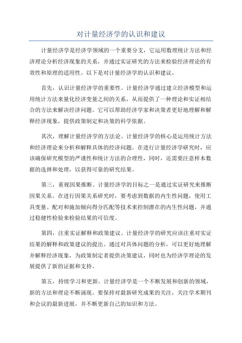
C5.1(1)代码:mydata<-read.csv("C:\\Users\\x1nreborn\\Desktop\\新建文件夹\\伍德里奇计量经济学导论第四版数据总和\\excel 伍德里奇\\wage1.csv", header=F,sep=",",stringsAsFactors=FALSE)wage<-mydata[,1:4]names(wage)<-c("wage","educ","exper","tenure")fit1<-lm(wage~educ+exper+tenure,data=wage)fit1summary(fit1)residual<-resid(fit1)hist(residual)结果:Coefficients:(Intercept) educ exper tenure -2.87273 0.59897 0.02234 0.16927 Residuals:Min 1Q Median 3Q Max-7.6068 -1.7747 -0.6279 1.1969 14.6536Histogram of residualresidual F r e q u e n c y-505101505010015020(2)代码:mydata<-read.csv("C:\\Users\\x1nreborn\\Desktop\\新建文件夹\\伍德里奇计量经济学导论第四版数据总和\\excel 伍德里奇\\wage1.csv", header=F,sep=",",stringsAsFactors=FALSE)wage<-mydata[,1:4]names(wage)<-c("wage","educ","exper","tenure")fit2<-lm(log(wage)~educ+exper+tenure,data=wage)fit2summary(fit2)residual2<-resid(fit2)hist(residual2)结果:Coefficients:(Intercept) educ exper tenure 0.284360 0.092029 0.004121 0.022067 Residuals:Min 1Q Median 3Q Max-2.05802 -0.29645 -0.03265 0.28788 1.42809Histogram of residual2residual2F r e q u e n c y-2-1105010015020(3)我认为对数—水平值模型更接近于满足假定MLR.6C5.2(1)代码:mydata<-read.csv("C:\\Users\\x1nreborn\\Desktop\\新建文件夹\\伍德里奇计量经济学导论第四版数据总和\\excel伍德里奇\\gpa2.csv",header=F,sep=",",stringsAsFactors=FALSE)gpa2<-mydata[,c(1,3,8)]names(gpa2)<-c("sat","colgpa","hsperc")fit<-lm(colgpa~hsperc+sat,data=gpa2)summary(fit)结果:Coefficients:(Intercept) hsperc sat1.391757 -0.013519 0.001476Coefficients:Estimate Std. Error t value Pr(>|t|)(Intercept) 1.392e+00 7.154e-02 19.45 <2e-16hsperc -1.352e-02 5.495e-04 -24.60 <2e-16sat 1.476e-03 6.531e-05 22.60 <2e-16(2)代码:gpa3<-gpa2[1:2070,]fit1<-lm(colgpa~hsperc+sat,data=gpa3)结果:Coefficients:(Intercept) hsperc sat1.436017 -0.012749 0.001468(3)c11=4.6 c12=0.0353 c13=0.0042c21=4.4 c22=0.0327 c23=0.00403所以c1i=c2i,可认为符合(5.10)中的等式。
C5.3mydata<-read.csv("C:\\Users\\x1nreborn\\Desktop\\新建文件夹\\伍德里奇计量经济学导论第四版数据总和\\excel伍德里奇\\bwght.csv",header=F,sep=",",stringsAsFactors=FALSE)bwght1<-mydata[,c(4,10,7,1,5,6)]names(bwght1)<-c("bwght","cigs","parity","faminc","motheduc","fathedu c")bwght1$motheduc[bwght1$motheduc=="."]<-NAbwght1$fatheduc[bwght1$fatheduc=="."]<-NAbwght2<-na.omit(bwght1)fit<-lm(bwght~cigs+parity+faminc+motheduc+fatheduc,data=bwght2)R<-residuals(fit)bwght2$R<-Rfit1<-lm(R~cigs+parity+faminc+motheduc+fatheduc,data=bwght2)结果显示,motheduc和fatheduc不联合显著。
C6.2(1)代码:mydata<-read.csv("C:\\Users\\x1nreborn\\Desktop\\新建文件夹\\伍德里奇计量经济学导论第四版数据总和\\excel伍德里奇\\wage1.csv",header=F,sep=",",stringsAsFactors=FALSE)wage<-mydata[,1:3]names(wage)<-c("wage","educ","exper")fit1<-lm(log(wage)~educ+exper+I(exper^2),data=wage)结果:Coefficients:(Intercept) educ exper I(exper^2)0.1279975 0.0903658 0.0410089 -0.0007136Coefficients:Estimate Std. Error t value Pr(>|t|)(Intercept) 0.1279975 0.1059323 1.208 0.227educ 0.0903658 0.0074680 12.100 < 2e-16exper 0.0410089 0.0051965 7.892 1.77e-14I(exper^2) -0.0007136 0.0001158 -6.164 1.42e-09(2)exper^2在1%的显著性水平上是显著的。
(3)工作五年,每多一年,工资上升3.387%工作二十年,每多一年,工资上升1.246%(4)exper取28.7年的时候,工作经历的增加实际上会降低预期的log(wage)样本中有121人具有比该取值更长的工作经历。
C6.3(1)对等式右边的educ求导,则可得b1+b3exper。
(2)对立假设为:教育的回报取决于exper的水平。
即b3!=0。
(3)代码:mydata<-read.csv("C:\\Users\\x1nreborn\\Desktop\\新建文件夹\\伍德里奇计量经济学导论第四版数据总和\\excel伍德里奇\\wage2.csv",header=F,sep=",",stringsAsFactors=FALSE)wage<-mydata[,c(1,5,6)]names(wage)<-c("wage","educ","exper")fit1<-lm(log(wage)~educ+exper+educ:exper,data=wage)fit1结果:Coefficients:Estimate Std. Error t value Pr(>|t|) (Intercept) 5.949455 0.240826 24.704 <2e-16educ 0.044050 0.017391 2.533 0.0115exper -0.021496 0.019978 -1.076 0.2822educ:exper 0.003203 0.001529 2.095 0.0365所以在5%的水平下,可以拒绝原假设,即可以认为教育的回报取决于exper的水平。
(4)b1的估计值为0.044,置信区间为[0.009136,0.078086]C7.1(1)代码:mydata<-read.csv("C:\\Users\\x1nreborn\\Desktop\\新建文件夹\\伍德里奇计量经济学导论第四版数据总和\\excel伍德里奇\\gpa1.csv",header=F,sep=",",stringsAsFactors=FALSE)gpa<-mydata[,c(10,11,12,19,28,29)]names(gpa)<-c("colGPA","hsGPA","ACT","PC","fathcoll","mothcoll")fit<-lm(colGPA~PC+hsGPA+ACT+mothcoll+fathcoll,data=gpa)结果:Coefficients:Estimate Std. Error t value Pr(>|t|) (Intercept) 1.255554 0.335392 3.744 0.000268PC 0.151854 0.058716 2.586 0.010762hsGPA 0.450220 0.094280 4.775 4.61e-06ACT 0.007724 0.010678 0.723 0.470687mothcoll -0.003758 0.060270 -0.062 0.950376fathcoll 0.041800 0.061270 0.682 0.496265拥有PC的估计影响有所降低,但它还是显著的(显著性水平为5%)(2)F=[(0.222-0.219)/2]/[(1-0.219)/135]=0.2593所以mothcoll和fathcoll联合不显著,p值为0.228(3)fit<-lm(colGPA~PC+hsGPA+ACT+mothcoll+fathcoll+I(hsGPA^2),data=gp a)结果: Estimate Std. Error t value Pr(>|t|)I(hsGPA^2) 0.337340 0.215710 1.564 0.1202因为p值大于0.05,所以接受原假设,没有必要进行增添平方项的扩展。