
统计学中的类型I和类型II错误
统计学中的类型I和类型II错误统计学是一门研究数据收集、分析和解释的学科。
在统计学中,我们经常会遇到两种不同的错误类型:类型I错误和类型II错误。
这两种错误类型在实际研究和决策过程中具有重要意义,本文将介绍统计学中的类型I和类型II错误,以及其对实践的影响。
一、类型I错误
类型I错误,又称为α错误,是指在进行假设检验时,拒绝了真实的无效假设(零假设)的错误。
换句话说,类型I错误发生时,我们错误地认为有一个关联或差异存在,而事实上并没有。
在统计学中,我们进行假设检验来判断样本数据是否支持或拒绝某一假设。
通常情况下,我们设置一个显著性水平(一般为0.05),当p 值小于显著性水平时,我们拒绝零假设,并得出结论。
然而,如果我们设置了过高的显著性水平或者在多次重复试验中进行了多重假设检验,那么就会增加犯下类型I错误的风险。
类型I错误可能会导致假阳性结果的产生。
例如,在药物实验中,如果我们错误地拒绝了药物对疾病没有治疗效果的零假设,那么我们可能会得出一个错误的结论,即认为该药物有效。
这可能导致不必要的治疗和资源浪费。
二、类型II错误
类型II错误,又称为β错误,是指未能拒绝无效假设(零假设)的错误。
换句话说,类型II错误发生时,我们无法检测到实际存在的关联或差异。
类型II错误通常与样本容量的大小有关。
当样本容量过小,检验的功效就会降低,从而导致类型II错误的风险增加。
另外,当效应大小较小或困难度较高时,也可能增加类型II错误的概率。
类型II错误可能会导致假阴性结果的出现。
例如,在临床试验中,如果我们未能拒绝一种药物无效的零假设,可能会导致需要治疗的患者无法获得有效的药物。
这可能延误或甚至危及患者的生命。
三、类型I和类型II错误对实践的影响
类型I和类型II错误的发生对实践都有重要影响。
过于关注避免类型I错误可能导致犯下更多的类型II错误,而过于关注避免类型II错误可能导致犯下更多的类型I错误。
在科学研究和医学实践中,我们需要在类型I和类型II错误之间寻找平衡点。
通常来说,我们需要根据具体情况来决定更关注哪一种错误类型。
例如,在一项临床试验中,如果有重大的副作用风险,我们可能更愿意接受类型I错误的风险,以确保患者的安全。
此外,准确估计和控制类型I和类型II错误的概率也非常重要。
我们可以通过增加样本容量、合理设置显著性水平、进行先进的统计模型等方式来降低这两种错误的概率。
同时,我们也应该意识到类型I和
类型II错误并非完全可以避免,我们只能在可控范围内尽量减少其发生的概率。
四、结论
统计学中的类型I和类型II错误是不可忽视的。
对这两种错误的理解和控制在科学研究、医学实践以及其他领域的决策中都非常重要。
我们需要充分认识并平衡类型I和类型II错误之间的关系,以便做出准确的结论和决策,并最大程度地减少错误带来的负面影响。
统计学中的假设检验误差控制

统计学中的假设检验误差控制概述统计学中的假设检验是一种常用的推断方法,用于判断样本数据与总体参数之间的关系。
然而,在进行假设检验时,存在两种类型的错误,即第一类错误和第二类错误,可能会对研究结论产生误导和不准确的结果。
因此,控制假设检验误差是十分重要的。
第一类错误第一类错误,也被称为α错误,指的是在实际上原假设为真的情况下,拒绝原假设的错误。
换句话说,我们拒绝了一个在统计上不存在的效应或关联关系。
第一类错误的概率通常称为显著性水平α,通常取0.05或0.01。
为了控制第一类错误,研究者可以通过调整显著性水平,降低拒绝原假设的概率。
然而,降低显著性水平会增加第二类错误的风险。
第二类错误第二类错误,也被称为β错误,指的是在实际上原假设为假的情况下,接受原假设的错误。
换句话说,我们未能发现一个实际上存在的效应或关联关系。
第二类错误的概率通常称为β,与样本大小、效应大小和显著性水平等因素有关。
为了控制第二类错误,研究者可以通过增加样本容量、选择更敏感的统计检验方法或减小假设检验中的误差界限等方式来降低第二类错误的风险。
然而,这也会增加研究的成本和时间消耗。
误差控制方法误差控制方法有多种,下面将介绍其中两种常用的方法:Bonferroni修正和Benjamin-Hochberg程序。
Bonferroni修正:Bonferroni修正是一种简单而直接的误差控制方法,它通过将显著性水平除以进行检验的总数量来调整显著性水平。
例如,当进行多个假设检验时,如果显著性水平α为0.05,而进行的假设检验数量为10个,则修正后的显著性水平为0.05/10=0.005。
这样做的目的是降低每个检验的显著性水平,以减少第一类错误的概率。
Benjamin-Hochberg程序:Benjamin-Hochberg程序是一种控制假设检验误差的多重比较方法,它通过比较每个检验的p值与经过排序和调整的显著性水平来确定拒绝或接受原假设。
该程序首先计算每个检验的p值,然后将p值进行排序,然后逐一比较每个检验的p值与调整后的显著性水平。
统计学中的假设检验错误类型

统计学中的假设检验错误类型统计学中的假设检验是一种常用的方法,用于推断总体参数或者判断两个总体是否有显著差异。
在进行假设检验时,我们通常会根据样本数据得出结论,但由于样本容量的限制和抽样误差的存在,假设检验也存在着一定的错误类型。
本文将介绍统计学中的假设检验错误类型,包括第一类错误和第二类错误。
一、第一类错误第一类错误,也被称为α错误或显著性水平错误,是指在实际上接受了错误的原假设。
即当原假设为真时,却错误地拒绝了原假设。
第一类错误的概率通常用α表示,它是我们在进行假设检验时所能容忍的拒绝原假设的错误概率。
当α的值较小时,我们对原假设要求越严格,也就是要求更高的证据才能拒绝原假设。
第一类错误的发生往往会引起不必要的亏损。
例如,在药物研究中,原假设是新药和对照组无差异,我们拒绝了原假设,即误认为新药比对照组更有效。
然而,实际上新药并没有带来明显的改善,这样就导致了开发者不必要的资金和时间损失。
因此,我们需要控制第一类错误的概率,以减少不必要的费用和资源浪费。
二、第二类错误第二类错误,也被称为β错误,是指在实际上拒绝了错误的原假设。
即当原假设为假时,却错误地接受了原假设。
第二类错误的概率通常用β表示,它是我们未能拒绝原假设的错误概率。
与第一类错误不同的是,我们无法直接控制第二类错误的概率,因为它与总体参数的真实值、样本容量和假设检验的效能有关。
第二类错误的发生往往会导致我们错过了重要的研究结果。
以制药业为例,假设我们想要证明新药的疗效优于对照组,原假设是两者无差异。
然而,由于样本容量不足或其他原因,我们无法拒绝原假设。
这样就可能导致我们未能发现新药的潜在疗效,从而影响到患者的治疗效果和药物研发的进展。
三、控制错误类型的方法为了控制第一类和第二类错误的概率,我们可以采取以下方法:1. 降低显著性水平:通过降低显著性水平α的取值,可以减少第一类错误的发生。
然而,较低的显著性水平也会导致第二类错误的概率增加。
统计学中的假设检验中的类型I和类型II错误

统计学中的假设检验中的类型I和类型II错误统计学中的假设检验是一种推断性统计方法,用于评估样本数据与所假设的总体参数之间的关系。
在进行假设检验时,我们通常会做出两种可能的错误判断,即类型I错误和类型II错误。
本文将详细介绍这两种错误及其在假设检验中的作用。
一、类型I错误类型I错误是指在原假设为真的情况下,拒绝原假设的错误判断。
换句话说,当实际上不存在显著差异时,我们错误地得出了存在显著差异的结论。
类型I错误的发生概率称为显著性水平(α),通常设置在0.01或0.05。
在假设检验中,我们会首先建立一个零假设(H0),即假设两个样本或总体没有差异。
然后通过计算样本数据的p值(或计算出来的显著性水平)来判断是否拒绝零假设。
如果p值小于设定的显著性水平,我们将拒绝零假设,并得出结论有显著差异。
然而,这种结论可能是错误的,即发生了类型I错误。
类型I错误的概率在理论上是可以控制的,通常通过设定显著性水平来控制。
较小的显著性水平可以减少类型I错误的概率,但也会增加类型II错误的概率。
二、类型II错误类型II错误是指在原假设为假的情况下,接受原假设的错误判断。
换句话说,当实际上存在显著差异时,我们未能得出存在显著差异的结论。
类型II错误的概率称为β,通常难以确定。
类型II错误的概率与样本大小、效应大小以及显著性水平等因素有关。
当样本大小较小时,可能存在较高的类型II错误概率。
当效应较小或显著性水平较高时,也会增加类型II错误的概率。
为了最小化类型II错误的概率,可以通过增加样本大小、明确效应大小以及适当选择显著性水平来进行调整。
三、平衡类型I和类型II错误在进行假设检验时,我们希望能够在保证控制类型I错误概率的同时,尽量减少类型II错误概率。
通常情况下,类型I错误概率(α)和类型II错误概率(β)是相互制约的。
当我们降低显著性水平以减少类型I错误时,往往会增加类型II错误的概率。
相反,若提高显著性水平以减少类型II错误,则可能会增加类型I错误的概率。
置信区间的I型错误和II型错误
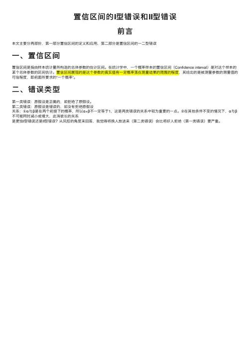
置信区间的I型错误和II型错误
前⾔
本⽂主要分两部份,第⼀部分置信区间的定义和应⽤,第⼆部分是置信区间的⼀⼆型错误
⼀、置信区间
置信区间是指由样本统计量所构造的总体参数的估计区间。
在统计学中,⼀个概率样本的置信区间(Confidence interval)是对这个样本的某个总体参数的区间估计。
置信区间展现的是这个参数的真实值有⼀定概率落在测量结果的周围的程度,其给出的是被测量参数的测量值的可信程度,即前⾯所要求的“⼀个概率”。
⼆、错误类型
第⼀类错误:原假设是正确的,却拒绝了原假设。
第⼆类错误:原假设是错误的,却没有拒绝原假设
关系:①α与β是在两个前提下的概率,所以α+β不⼀定等于1,这是两类错误的关系中较为重要的⼀点。
②在其他条件不变的情况下,α与β不可能同时减⼩或增⼤,此消彼长的关系
是更怕I型错误还是II型错误?从风控的⾓度来回答,我觉得将换⼈放进来(第⼆类错误)会⽐将好⼈拒绝(第⼀类错误)要严重。
统计推断中的I型错误和II型错误是什么

统计推断中的I型错误和II型错误是什么在统计学中,当我们进行统计推断时,常常会面临两种类型的错误,即 I 型错误和 II 型错误。
这两种错误对于我们正确理解和解释统计结果至关重要。
首先,让我们来了解一下什么是 I 型错误。
简单来说,I 型错误也被称为“假阳性错误”或“α错误”。
想象一下,我们正在进行一项假设检验,比如检验一种新药物是否有效。
我们先提出一个零假设(通常表示没有效果或没有差异),然后通过收集数据来判断是否有足够的证据拒绝这个零假设。
但有时候,尽管实际上零假设是正确的(也就是说新药物确实没有效果),但由于样本的随机性或者其他因素,我们却错误地拒绝了零假设,得出了药物有效的结论。
这就像是法官在审判一个实际上无罪的人时,却误判他有罪。
这种错误就是 I 型错误。
为了控制 I 型错误的发生概率,我们通常会设定一个显著性水平(通常用α表示)。
例如,如果我们将显著性水平设定为 005,这意味着我们愿意接受 5%的可能性犯 I 型错误。
也就是说,在 100 次假设检验中,平均可能会有 5 次错误地拒绝了实际上正确的零假设。
接下来,我们再看看 II 型错误。
II 型错误也被称为“假阴性错误”或“β错误”。
还是以新药物的检验为例,如果新药物实际上是有效的,但我们的检验结果却没能发现这一点,接受了零假设(即认为药物无效),那么这就是 II 型错误。
这就好比法官在审判一个实际上有罪的人时,却误判他无罪。
II 型错误的发生概率受到多种因素的影响。
其中一个重要的因素是样本量。
通常情况下,样本量越大,我们越有可能发现真实的差异或效果,从而减少 II 型错误的发生概率。
另一个影响因素是效应大小。
如果实际的效应很大,我们更容易检测到,II 型错误的概率就会降低;反之,如果效应较小,就更难检测到,II 型错误的概率就会增加。
那么,I 型错误和 II 型错误之间有什么关系呢?它们之间存在一种权衡关系。
一般来说,如果我们想要减少 I 型错误的概率(降低α),那么往往会增加 II 型错误的概率(增加β);反之,如果我们想要减少 II 型错误的概率,可能就需要增加 I 型错误的概率。
类型II错误及功效与抽样检验

类型 II 错误及功效与抽样检验1. 引言在统计学中,抽样检验是一种通过对样本数据进行分析来进行统计推断的方法。
抽样检验可用来验证假设,并确定一个事件是否发生的概率。
在进行抽样检验时,我们常常关注两种类型的错误:类型 I 错误和类型 II 错误。
本文将重点介绍类型 II 错误及其功效与抽样检验的关系。
2. 类型 II 错误的定义类型 II 错误是指在进行抽样检验时,未能拒绝一个错误的零假设的概率。
换句话说,类型 II 错误意味着我们未能发现一个真实的效果或差异。
类型 II 错误的概率通常用β 表示。
3. 增加功效以减少类型 II 错误为了减小类型 II 错误的概率,我们可以增加检验的功效。
检验的功效是指在一个真实效应存在时,正确地拒绝零假设的概率。
功效通常用 1- β 表示,其中β 是类型 II 错误的概率。
如何增加功效呢?以下是一些常用的方法:3.1 增加样本容量增加样本容量可以提高抽样检验的功效。
较大的样本容量意味着更接近总体情况的样本数据。
通过增加样本容量,我们可以更准确地估计总体的特征,并从而提高检验的功效。
3.2 减小显著性水平显著性水平(α)指的是在进行抽样检验时拒绝零假设的标准。
通常情况下,显著性水平取值为 0.05 或 0.01。
在一定程度上,减小显著性水平有助于减少类型 I 错误的概率,但也会增加类型 II 错误的概率。
因此,适当地选择显著性水平可以平衡两种错误的概率,提高抽样检验的功效。
3.3 增加效应大小效应大小是指总体之间的差异或关系的程度。
较大的效应大小意味着通过抽样检验更容易检测到这种差异。
因此,我们可以通过增加效应大小来提高检验的功效。
3.4 选择合适的检验方法选择合适的统计检验方法也可以影响抽样检验的功效。
不同的检验方法对不同类型的数据和假设有不同的适用性。
因此,选择合适的检验方法可以提高检验的功效。
4. 抽样检验的步骤进行抽样检验时,一般需要按照以下步骤进行:4.1 建立假设首先,我们需要建立一个原假设(零假设)和一个备择假设。
统计学中的假设检验错误类型分析
统计学中的假设检验错误类型分析假设检验是统计学的重要理论之一,用于判断样本数据对某个总体假设的支持度。
在假设检验过程中,我们会遇到两种类型的错误,即第一类错误和第二类错误。
本文将对这两种错误类型进行分析,并探讨如何降低错误率。
1. 第一类错误第一类错误也被称为显著性水平(Significance Level)或α错误。
它指的是在原假设为真的情况下,拒绝原假设的错误判断。
在假设检验中,我们通常会设定一个显著性水平来进行决策,常见的显著性水平有0.05和0.01。
当结果的p值小于设定的显著性水平时,我们将拒绝原假设。
然而,这种判断并不是绝对准确的,存在一定概率犯下错误。
第一类错误的概率通常用α表示。
当我们将显著性水平设定为0.05时,即α=0.05,意味着有5%的可能犯下第一类错误。
如果显著性水平设定得较低,例如α=0.01,那么犯第一类错误的概率将更小,但同时也会增加犯第二类错误的概率。
2. 第二类错误第二类错误是在原假设为假的情况下,接受原假设的错误判断。
与第一类错误相反,第二类错误常用β表示。
第二类错误的概率与样本大小、效应大小和显著性水平等因素有关。
当样本大小较小时,相同效应大小下犯第二类错误的概率较高;当效应大小较小时,相同样本大小下犯第二类错误的概率也较高;而当显著性水平设定较低时,犯第二类错误的概率也会增加。
3. 降低错误率的方法在实际应用中,我们希望尽可能降低第一类错误和第二类错误的概率,提高假设检验的准确性。
以下是一些常用的方法:3.1 增加样本容量通过增加样本容量,可以降低第一类错误和第二类错误的概率。
较大的样本容量能够提供更充分的信息,减小抽样误差,提高判断结果的准确性。
在样本容量不足时,可能会导致犯下更多的错误。
3.2 提高显著性水平设定较低的显著性水平可以降低第一类错误的概率。
但需要注意的是,过低的显著性水平会增加犯第二类错误的概率,因此需要权衡选择适当的显著性水平。
3.3 增大效应大小提高研究中的效应大小可以降低第二类错误的概率。
统计学知识(一类错误和二类错误)
Type I and type II errors(α) the error of rejecting a "correct" null hypothesis, and(β) the error of not rejecting a "false" null hypothesisIn 1930, they elaborated on these two sources of error, remarking that "in testing hypotheses two considerations must be kept in view, (1) we must be able to reduce the chance of rejecting a true hypothesis to as low a value as desired; (2) the test must be so devised that it will reject the hypothesis tested when it is likely to be false"[1]When an observer makes a Type I error in evaluating a sample against its parent population, s/he is mistakenly thinking that a statistical difference exists when in truth there is no statistical difference (or, to put another way, the null hypothesis is true but was mistakenly rejected). For example, imagine that a pregnancy test has produced a "positive" result (indicating that the woman taking the test is pregnant); if the woman is actually not pregnant though, then we say the test produced a "false positive". A Type II error, or a "false negative", is the error of failing to reject a null hypothesis when the alternative hypothesis is the true state of nature. For example, a type II error occurs if a pregnancy test reports "negative" when the woman is, in fact, pregnant.Statistical error vs. systematic errorScientists recognize two different sorts of error:[2]Statistical error: Type I and Type IIStatisticians speak of two significant sorts of statistical error. The context is that there is a "null hypothesis" which corresponds to a presumed default "state of nature", e.g., that an individual is free of disease, that an accused is innocent, or that a potential login candidate is not authorized. Corresponding to the null hypothesis is an "alternative hypothesis" which corresponds to the opposite situation, that is, that the individual has the disease, that the accused is guilty, or that the login candidate is an authorized user. Thegoal is to determine accurately if the null hypothesis can be discarded in favor of the alternative. A test of some sort is conducted (a blood test, a legal trial, a login attempt), and data is obtained. The result of the test may be negative (that is, it does not indicate disease, guilt, or authorized identity). On the other hand, it may be positive (that is, it may indicate disease, guilt, or identity). If the result of the test does not correspond with the actual state of nature, then an error has occurred, but if the result of the test corresponds with the actual state of nature, then a correct decision has been made. There are two kinds of error, classified as "Type I error" and "Type II error," depending upon which hypothesis has incorrectly been identified as the true state of nature.Type I errorType I error, also known as an "error of the first kind", an α error, or a "false positive": the error of rejecting a null hypothesis when it is actually true. Plainly speaking, it occurs when we are observing a difference when in truth there is none. Type I error can be viewed as the error of excessive skepticism.Type II errorType II error, also known as an "error of the second kind", a βerror, or a "false negative": the error of failing to reject a null hypothesis when it is in fact false. In other words, this is the error of failing to observe a difference when in truth there is one. Type II error can be viewed as the error of excessive gullibility.See Various proposals for further extension, below, for additional terminology.Understanding Type I and Type II errorsHypothesis testing is the art of testing whether a variation between two sample distributions can be explained by chance or not. In many practical applications Type I errors are more delicate than Type II errors. In these cases, care is usually focused on minimizing the occurrence of this statistical error. Suppose, the probability for a Type I error is 1% or 5%, then there is a 1% or 5% chance that the observed variation is not true. This is called the level of significance. While 1% or 5% might be an acceptable level of significance for one application, a different application can require a very different level. For example, the standard goal of six sigma is to achieve exactness by 4.5 standard deviations above or below the mean. That is, for a normally distributed process only 3.4 parts per million are allowed to be deficient. The probability of Type I error is generally denoted with the Greek letter alpha.In more common parlance, a Type I error can usually be interpreted as a false alarm, insufficient specificity or perhaps an encounter with fool's gold. A Type II error could be similarly interpreted as an oversight, a lapse in attention or inadequate sensitivity.EtymologyIn 1928, Jerzy Neyman (1894-1981) and Egon Pearson (1895-1980), both eminent statisticians, discussed the problems associated with "deciding whether or not a particular sample may bejudged as likely to have been randomly drawn from a certain population" (1928/1967, p.1): and, as Florence Nightingale David remarked, "it is necessary to remember the adjective ‘random’ [in the term ‘random sample’] should apply t o the method of drawing the sample and not to the sample itself" (1949, p.28).They identified "two sources of error", namely:(a) the error of rejecting a hypothesis that should have been accepted, and(b) the error of accepting a hypothesis that should have been rejected (1928/1967, p.31). In 1930, they elaborated on these two sources of error, remarking that:…in testing hypotheses two considerations must be kept in view, (1) we must be able to reduce the chance of rejecting a true hypothesis to as low a value as desired; (2) the test must be so devised that it will reject the hypothesis tested when it is likely to be false (1930/1967, p.100).In 1933, they observed that these "problems are rarely presented in such a form that we can discriminate with certainty between the true and false hypothesis" (p.187). They also noted that, in deciding whether to accept or reject a particular hypothesis amongst a "set of alternative hypotheses" (p.201), it was easy to make an error:…[and] these errors will be of two kinds:(I) we reject H[i.e., the hypothesis to be tested] when it is true,(II) we accept H0when some alternative hypothesis Hiis true. (1933/1967, p.187)In all of the papers co-written by Neyman and Pearson the expression Halways signifies "the hypothesis to be tested" (see, for example, 1933/1967, p.186).In the same paper[4] they call these two sources of error, errors of type I and errors of type II respectively.[5]Statistical treatmentDefinitionsType I and type II errorsOver time, the notion of these two sources of error has been universally accepted. They are now routinely known as type I errors and type II errors. For obvious reasons, they are very often referred to as false positives and false negatives respectively. The terms are now commonly applied in much wider and far more general sense than Neyman and Pearson's original specific usage, as follows:Type I errors (the "false positive"): the error of rejecting the null hypothesis given that it is actually true; e.g., A court finding a person guilty of a crime that they did not actually commit.Type II errors(the "false negative"): the error of failing to reject the null hypothesis given that the alternative hypothesis is actually true; e.g., A court finding a person not guilty of a crime that they did actually commit.These examples illustrate the ambiguity, which is one of the dangers of this wider use: They assume the speaker is testing for guilt; they could also be used in reverse, as testing for innocence; or two tests could be involved, one for guilt, the other for innocence. (This ambiguity is one reason for the Scottish legal system's third possible verdict: not proven.)The following tables illustrate the conditions.Example, using infectious disease test results:Example, testing for guilty/not-guilty:Example, testing for innocent/not innocent – sense is reversed from previous example:Note that, when referring to test results, the terms true and false are used in two different ways: the state of the actual condition (true=present versus false=absent); and the accuracy or inaccuracy of the test result (true positive, false positive, true negative, false negative). This is confusing to some readers. To clarify the examples above, we have used present/absent rather than true/false to refer to the actual condition being tested.False positive rateThe false positive rate is the proportion of negative instances that were erroneously reported as being positive.It is equal to 1 minus the specificity of the test. This is equivalent to saying the false positive rate is equal to the significance level.[6]It is standard practice for statisticians to conduct tests in order to determine whether or not a "speculative hypothesis" concerning the observed phenomena of the world (or its inhabitants) can be supported. The results of such testing determine whether a particular set of results agrees reasonably (or does not agree) with the speculated hypothesis.On the basis that it is always assumed, by statistical convention, that the speculated hypothesis is wrong, and the so-called "null hypothesis" that the observed phenomena simply occur by chance (and that, as a consequence, the speculated agent has no effect) — the test will determine whether this hypothesis is right or wrong. This is why the hypothesis under test is often called the null hypothesis (most likely, coined by Fisher (1935, p.19)), because it is this hypothesis that is to be either nullified or not nullified by the test. When the null hypothesis is nullified, it is possible to conclude that data support the "alternative hypothesis" (which is the original speculated one).The consistent application by statisticians of Neyman and Pearson's convention of representing "the hypothesis to be tested" (or "the hypothesis to be nullified") with the expression H0has led to circumstances where many understand the term "the null hypothesis" as meaning "the nil hypothesis" — a statement that the results in question have arisen through chance. This is not necessarily the case — the key restriction, as per Fisher (1966), is that "the null hypothesis must be exact, that is free from vagueness and ambiguity, because it must supply the basis of the 'problem of distribution,' of which the test of significance is the solution."[9] As a consequence of this, in experimental science the null hypothesis is generally a statement that a particular treatment has no effect; in observational science, it is that there is nodifference between the value of a particular measured variable, and that of an experimental prediction.The extent to which the test in question shows that the "speculated hypothesis" has (or has not) been nullified is called its significance level; and the higher the significance level, the less likely it is that the phenomena in question could have been produced by chance alone. British statistician Sir Ronald Aylmer Fisher(1890–1962) stressed that the "null hypothesis":…is never proved or established, but is possibly disproved, in the course ofexperimentation. Every experiment may be said to exist only in order to give the factsa chance of disproving the null hypothesis. (1935, p.19)Bayes's theoremThe probability that an observed positive result is a false positive (as contrasted with an observed positive result being a true positive) may be calculated using Bayes's theorem.The key concept of Bayes's theorem is that the true rates of false positives and false negatives are not a function of the accuracy of the test alone, but also the actual rate or frequency of occurrence within the test population; and, often, the more powerful issue is the actual rates of the condition within the sample being tested.Various proposals for further extensionSince the paired notions of Type I errors(or "false positives") and Type II errors(or "false negatives") that were introduced by Neyman and Pearson are now widely used, their choice of terminology ("errors of the first kind" and "errors of the second kind"), has led others to suppose that certain sorts of mistake that they have identified might be an "error of the third kind", "fourth kind", etc.[10]None of these proposed categories have met with any sort of wide acceptance. The following is a brief account of some of these proposals.DavidFlorence Nightingale David (1909-1993),[3] a sometime colleague of both Neyman and Pearson at the University College London, making a humorous aside at the end of her 1947 paper, suggested that, in the case of her own research, perhaps Neyman and Pearson's "two sources of error" could be extended to a third:I have been concerned here with trying to explain what I believe to be the basic ideas[of my "theory of the conditional power functions"], and to forestall possible criticism that I am falling into error (of the third kind) and am choosing the test falsely to suit the significance of the sample. (1947), p.339)MostellerIn 1948, Frederick Mosteller (1916-2006)[11] argued that a "third kind of error" was required to describe circumstances he had observed, namely:∙Type I error: "rejecting the null hypothesis when it is true".∙Type II error: "accepting the null hypothesis when it is false".∙Type III error: "correctly rejecting the null hypothesis for the wrong reason". (1948, p.61)KaiserIn his 1966 paper, Henry F. Kaiser (1927-1992) extended Mosteller's classification such that an error of the third kind entailed an incorrect decision of direction following a rejected two-tailed test of hypothesis. In his discussion (1966, pp.162-163), Kaiser also speaks of α errors, β errors, and γ errors for type I, type II and type III errors respectively.KimballIn 1957, Allyn W. Kimball, a statistician with the Oak Ridge National Laboratory, proposed a different kind of error to stand beside "the first and second types of error in the theory of testing hypotheses". Kimball defined this new "error of the third kind" as being "the error committed by giving the right answer to the wrong problem" (1957, p.134).Mathematician Richard Hamming (1915-1998) expressed his view that "It is better to solve the right problem the wrong way than to solve the wrong problem the right way".The famous Harvard economist Howard Raiffa describes an occasion when he, too, "fell into the trap of working on the wrong problem" (1968, pp.264-265).[12]Mitroff and FeatheringhamIn 1974, Ian Mitroff and Tom Featheringham extended Kimball's category, arguing that "one of the most important determinants of a problem's solution is how that problem has been represented or formulated in the first place".They defined type III errors as either "the error… of having solved the wrong problem… when one should have solved the right problem" or "the error… [of] choosing the wrong problem representation… when one should have… chosen the right problem representation" (1974), p.383).RaiffaIn 1969, the Harvard economist Howard Raiffa jokingly suggested "a candidate for the error of the fourth kind: solving the right problem too late" (1968, p.264).Marascuilo and LevinIn 1970, Marascuilo and Levin proposed a "fourth kind of error" -- a "Type IV error" -- which they defined in a Mosteller-like manner as being the mistake of "the incorrect interpretation of a correctly rejected hypothesis"; which, they suggested, was the equivalent of "a physician's correct diagnosis of an ailment followed by the prescription of a wrong medicine" (1970, p.398).Usage examplesStatistical tests always involve a trade-off between:(a) the acceptable level of false positives (in which a non-match is declared to be amatch) and(b) the acceptable level of false negatives (in which an actual match is not detected).A threshold value can be varied to make the test more restrictive or more sensitive; with the more restrictive tests increasing the risk of rejecting true positives, and the more sensitive tests increasing the risk of accepting false positives.ComputersThe notions of "false positives" and "false negatives" have a wide currency in the realm of computers and computer applications.Computer securitySecurity vulnerabilities are an important consideration in the task of keeping all computer data safe, while maintaining access to that data for appropriate users (see computer security, computer insecurity). Moulton (1983), stresses the importance of:∙avoiding the type I errors (or false positive) that classify authorized users as imposters.∙avoiding the type II errors (or false negatives) that classify imposters as authorized users (1983, p.125).False Positive (type I) -- False Accept Rate (FAR) or False Match Rate (FMR)False Negative (type II) -- False Reject Rate (FRR) or False Non-match Rate (FNMR)The FAR may also be an abbreviation for the false alarm rate, depending on whether the biometric system is designed to allow access or to recognize suspects. The FAR is considered to be a measure of the security of the system, while the FRR measures the inconvenience level for users. For many systems, the FRR is largely caused by low quality images, due to incorrect positioning or illumination. The terminology FMR/FNMR is sometimes preferred to FAR/FRR because the former measure the rates for each biometric comparison, while the latter measure the application performance (ie. three tries may be permitted).Several limitations should be noted for the use of these measures for biometric systems:(a) The system performance depends dramatically on the composition of the test database(b) The system performance measured in this way is the zero-effort error rate. Attackersprepared to use active techniques such as spoofing will decrease FAR.(c) Such error rates only apply properly to biometric verification (or one-to-onematching)systems. The performance of biometric identification or watch-list systems is measured with other indices (such as the cumulative match curve (CMC))∙Screening involves relatively cheap tests that are given to large populations, none of whom manifest any clinical indication of disease (e.g., Pap smears).∙Testing involves far more expensive, often invasive, procedures that are given only to those who manifest some clinical indication of disease, and are most often applied to confirm a suspected diagnosis.test a population with a true occurrence rate of 70%, many of the "negatives" detected by the test will be false. (See Bayes' theorem)False positives can also produce serious and counter-intuitive problems when the condition being searched for is rare, as in screening. If a test has a false positive rate of one in ten thousand, but only one in a million samples (or people) is a true positive, most of the "positives" detected by that test will be false.[17]Paranormal investigationThe notion of a false positive has been adopted by those who investigate paranormal or ghost phenomena to describe a photograph, or recording, or some other evidence that incorrectly appears to have a paranormal origin -- in this usage, a false positive is a disproven piece of media "evidence" (image, movie, audio recording, etc.) that has a normal explanation.[18]。
假设检验中的第一类错误和第二类错误
假设检验中的第一类错误和第二类错误假设检验是统计学中常用的一种方法,用于评估研究者对于一个假设的推断是否正确。
在进行假设检验时,我们常常会面临两种类型的错误,即第一类错误和第二类错误。
了解这两种错误的含义和影响,对于正确理解假设检验的结果和取得可靠的研究结论非常重要。
一、第一类错误第一类错误,又被称为显著性水平α水平的错误,是指在实际情况为真的情况下,拒绝了原假设的错误判断。
换句话说,第一类错误意味着我们错误地推断出了一种不存在的效应或关系。
在假设检验中,我们通常会设置一个显著性水平(α)作为拒绝原假设的标准。
常见的显著性水平为0.05或0.01。
如果计算得出的p值小于设定的显著性水平,我们就会拒绝原假设。
然而,这样的判断并不意味着我们完全排除了第一类错误的风险。
事实上,在大量研究中使用统计显著性水平为0.05的情况下,仍有5%的概率犯下第一类错误。
举个例子来说,假设我们正在研究一个新的药物对于疾病的治疗效果,我们的原假设是该药物无效。
经过数据分析后,我们得到了一个p 值为0.03,小于我们设定的显著性水平0.05。
根据这一结果,我们拒绝了原假设,认为该药物具有疗效。
然而,事实上,该药物可能并没有真正的治疗效果,我们此时实际上犯下了第一类错误。
第一类错误的发生可能会导致严重的后果。
例如,一个错误地认为某种药物有治疗效果,导致该药物被广泛应用,却最终证明该药物的副作用或无效,由此给患者带来不良影响。
因此,我们在进行假设检验时,需要权衡显著性水平的选择,降低第一类错误的风险。
二、第二类错误第二类错误是指在实际情况为假的情况下,接受了原假设的错误判断。
换句话说,第二类错误意味着我们无法检测到真实存在的效应或关系。
在假设检验中,我们设定了拒绝原假设的显著性水平,但并没有设定接受原假设的显著性水平。
因此,在数据分析中,我们不能直接得出不存在关系的结论,而只能得到数据不足以拒绝原假设的结论。
因此,第二类错误的概率通常由实验者根据研究设计确定。
i类误差和ii类误差
i类误差和ii类误差I 类误差和 II 类误差引言:在统计学中,我们经常需要进行各种类型的假设检验。
在这些检验中,我们通常会犯两种类型的错误,即 I 类误差和 II 类误差。
本文将详细介绍这两种错误的定义、原因、影响以及如何最小化它们。
一、I 类误差1. 定义:I 类误差也被称为“虚假阳性”或“α错误”。
它指的是在原假设为真时拒绝了原假设的情况。
2. 原因:I 类误差通常是由于样本数据产生的随机变异或实验设计不合理导致的。
过于宽松的显著性水平(α)也可能导致增加I 类错误发生的概率。
3. 影响:发生 I 类错误会导致我们错误地拒绝了一个真实的假设,即得出了一个虚假阳性结果。
这可能引起不必要的麻烦和浪费资源。
4. 最小化 I 类误差:为了最小化 I 类错误,我们可以采取以下措施:- 合理设计实验:确保实验设计符合科学原则,并尽量减少潜在影响结果的干扰因素。
- 选择适当的显著性水平:根据研究领域和问题的重要性,选择一个合适的显著性水平来控制 I 类错误的概率。
- 增加样本容量:通过增加样本容量可以减少随机误差对结果的影响,从而降低 I 类错误的概率。
二、II 类误差1. 定义:II 类误差也被称为“虚假阴性”或“β错误”。
它指的是在原假设为假时接受了原假设的情况。
2. 原因:II 类误差通常是由于样本数据不足或实验设计不合理导致的。
过于严格的显著性水平(α)也可能导致增加 II 类错误发生的概率。
3. 影响:发生 II 类错误会导致我们未能拒绝一个错误的假设,即得出了一个虚假阴性结果。
这可能导致错失发现真实效应或关联关系的机会。
4. 最小化 II 类误差:为了最小化 II 类错误,我们可以采取以下措施:- 增加样本容量:通过增加样本容量可以提高研究统计功效,从而减少 II 类错误的概率。
- 选择适当的显著性水平:根据研究领域和问题的重要性,选择一个合适的显著性水平来控制 II 类错误的概率。
- 使用更敏感的测量工具:选择更敏感的测量工具可以增加检测到真实效应或关联关系的机会。